Optimizing subclass Discriminant Error Correcting Output Codes
using Particle Swarm Optimization
Dimitrios Bouzas, Nikolaos Arvanitopoulos and Anastasios Tefas
Department of Informatics, Aristotle University of ThessalonikiBox 451, 54124 Thessaloniki, Greece,
{dmpouzas, niarvani}@csd.auth.gr, [email protected]
Abstract—Error-Correcting Output Codes (ECOC) reveal a common way to model multi-class classification problems. According to this state of the art technique, a multi-class problem is decomposed into several binary ones. Additionally, on the ECOC framework we can apply thesubclass technique (sub-ECOC), where by splitting the initial classes of the problem we create larger but easier to solve ECOC configurations. The multi-class problem’s decomposition is achieved via a discriminant tree creation procedure. This discriminant tree’s creation is controlled by a triplet of thresholds that define a set of user defined splitting standards. The selection of the thresholds plays a major role in the classification performance. In our work we show that by optimizing these thresholds via particle swarm optimization we improve significantly the classification performance. Moreover, using Support Vector Machines (SVMs) as classifiers we can optimize in the same time both the thresholds of sub-ECOC and the parameters C and σ of the SVMs, resulting in even better classification performance. Extensive experiments in both real and artificial data illustrate the superiority of the proposed approach in terms of performance.
I. INTRODUCTION
In the literature one can find various binary classification techniques. However, in the real world the problems to be addressed are usually class. In dealing with multi-class problems we must use the binary techniques as a leverage. This can be achieved by defining a method that decomposes the multi-class problem into several binary ones, and combines their solutions to solve the initial multi-class problem [6]. In this context, the Error-Correcting Output Codes (ECOC) emerged. Based on the error correcting principles [5] and on its ability to correct the bias and variance errors of the base classifiers [10], this state of the art technique has been proved valuable in solving multi-class multi-classification problems over a number of fields and applications.
As proposed by Escalera et al., on the ECOC framework we can apply the subclass technique [1]. According to this technique, we use a guided problem dependent procedure to group the classes and split them into subsets with respect to the improvement we obtain in the training performance. This splitting is controlled via a set of thresholds. The selection of these thresholds has a major impact in the classification performance of the technique. In this paper we show that by optimizing these set of thresholds withparticle swarm optimization (PSO) we can boost the classification
performance.
In our experiments we used the support vector machine with linear and RBF kernels as a standard classifier [4] and applied it on 8 multi-class learning problems provided by the UCI machine learning repository [22] and 4 artificially created datasets. In parallel with the optimization of the above mentioned thresholds we also optimized with PSO the SVM’s parameters C and σ. Thus, we propose the use of PSO as an efficient and fast optimization technique of complex classifiers.
The paper is organized as follows: A brief introduction to the ECOC framework is given in Section II. The sub-ECOC technique is described in Section III. The loss weighted decodingtechnique is illustrated in Section IV. A description of the sequential forward floating search (SFFS) algorithm is given in Section V. Thefast quadratic mutual information (FQMI) procedure used to model the mutual information between classes is analyzed in Section VI. A description of the PSO algorithm and its variations is given in Section VII. The configuration we used in our experiments is described in Section VIII. Our experimental results are illustrated in Section IX. Finally, in Section X we conclude our work.
II. ERRORCORRECTINGOUTPUTCODES
ECOC is a general framework to solve multi-class prob-lems by decomposing them into several binary ones. This technique consists of two separate steps: a) theencodingand b) thedecodingstep [2].
a) In the encoding step, given a set of N classes, we assign a unique binary string called codeword (i.e., a sequence of bits of a code representing each class, where each bit identifies the membership of the class for a given binary classifier) to each class. The length
n of each codeword represents the number of bi-partitions (i.e., groups of classes) that are formed and, consequently, the number of binary problems to be trained. Each bit of the codeword represents the response of the corresponding binary classifier and it is coded by +1 or -1, according to its class membership. The next step is to arrange all these codewords as rows of a matrix obtaining the so-calledcoding matrix
M, where M ∈ {−1,+1}N×n. Each column of this
defines the membership of the corresponding class in the specific binary problem.
An extension of this standard ECOC approach was proposed by Allwein et al. by adding a third symbol in the coding process [6]. The new coding matrix M is nowM∈ {−1,0,+1}N×n. In this approach, the zero
symbol means that a certain class is not considered by a specific binary classifier. As a result, this symbol increases the number of bi-partitions to be created in the ternary ECOC framework.
b) The decoding step of the ECOC approach consists of applying thendifferent binary classifiers to each data sample in the test set, in order to obtain a code for this sample. This code is then compared to all the codewords of the classes defined in the coding matrix
M and the sample is assigned to the class with the closest codeword. The most frequently used decoding methods are theHammingand theEuclideandecoding distances.
III. SUB-ECOC
Escalera et al. proposed that from an initial set of classes Cof a given multi-class problem, we can define a new set of classes C0, where the cardinality ofC0 is greater than that of C, that is|C0|>|C|[1]. The new set of binary problems that will be created will improve the created classifiers’ training performance. Additionally to the ECOC framework, Pujol proposed that we can use a ternary problem dependent design of ECOC, calleddiscriminant ECOC (DECOC)where, given a number ofN classes, we can achieve a high classification performance by training onlyN−1binary classifiers [3]. The combination of the above mentioned methods results in a new classification procedure called sub-ECOC. The procedure is based on the creation of discriminant tree structures which depend on the problem domain.
These binary trees are built by choosing the problem partitioning that maximizes the MI between the samples and their respective class labels. The structure as a whole describes the decomposition of the initial multi-class problem into an assembly of smaller binary sub-problems. Each node of the tree represents a pair that consists of a specific binary sub-problem with its respective classifier. The construction of the tree’s nodes is achieved through an evaluation procedure [1]. According to this procedure, we can split the bi-partitions that consist the current sub-problem examined. Splitting can be achieved using K-means or some other clustering method. After splitting, we form two new problems that can be exam-ined separately. On each one of the new problems created, we repeat the SFFS procedure independently in order to form two new separate sub-problem domains that are easier to solve. Next, we evaluate the two new problem configurations against three user defined thresholds {θperf, θsize, θimpr}
described below. If the thresholds are satisfied, the new created pair of sub-problems is accepted along with their new created binary classifiers, otherwise they are rejected and we keep the initial configuration with its respective binary classifier.
• θperf: Split the classes if the created classifier attains
greater than θperf% training error.
• θsize: Minimum cluster’s size of an arbitrary created
subclass.
• θimpr: Improvement in the training error attained by
classifiers for the newly created problems against pre-vious classifier (before splitting).
IV. LOSS-WEIGHTEDDECODING
In the decoding process of the sub-ECOC approach we use the Loss Weighted Decoding algorithm [2]. As already mentioned, the 0 symbol in the decoding matrix allows to increase the number of binary problems created and as a result the number of different binary classifiers to be trained. Standard decoding techniques, such as the Euclidean or the Hamming distance do not consider this third symbol and often produce non-robust results. So, in order to solve the problems produced by the standard decoding algorithms, the loss weighted decoding was proposed.
The loss weighted decoding algorithm is summarized in Algorithm 1.
Algorithm 1 Loss Weighted Decoding Algorithm
Calculate Hypothesis matrix H
H(i, j) = 1 |Ji| P|Ji| k=1γ(hj(Jik), i, j) based on γ(xj, i, j) = 1 ifxj=M(i, j) 0 otherwise (1) NormalizeH so thatPn j=1MW(i, j) = 1, ∀i= 1, . . . , N: MW(i, j) = H(i, j) Pn j=1H(i, j) ,∀i∈[1, . . . , N], ∀j∈[1, . . . , n] (2) Given a test input℘, decode based on:
d(x, i) = n X j=1
−M(i, j)·hj(x)·MW(i, j) (3)
Obtain the final classcx for samplexby:
Ci∗: (i∗, j∗) = arg min
(i0j0)d(x,(i
0
j0)), C(i0j0)∈C0 (4)
The main objective is to define a weighting matrix MW
that weights a loss function to adjust the decision of the classifiers. In order to obtain the matrix MW, a hypothesis
matrix H is constructed first. The elements H(i, j) of this matrix are continuous values that correspond to the accuracy of the binary classifierhj classifying the samples of classi.
The matrixH has zero values in the positions which corre-spond to unconsidered classes, since these positions do not contain any representative information. The next step is the normalization of the rows of matrixH. By this normalization, the matrix MW can be considered as a discrete probability
density function. This is very important, since we assume that the probability of considering each class for the final classification is the same. Finally, we decode by computing
the weighted sum of our coding matrix M and our binary classifier with the weighting matrixMW and assign our test
sample to the class that attains the minimumdecoding value. V. SEQUENTIALFORWARDFLOATINGSEARCH The Floating search methods are a family of suboptimal sequential search methods that were developed as an alterna-tive counterpart to the more computational costly exhausalterna-tive search methods. These methods allow the search criterion to be non-monotonic. They are also able to counteract the nesting effect by considering conditional inclusion and exclusion of features controlled by the value of the criterion itself. In our approach we use a variation of the Sequential Forward Floating Search (SFFS) algorithm [8]. The SFFS method is described in Algorithm 2.
Algorithm 2 SFFS for Classes 1: Input:
2: Y ={yj|j= 1, . . . , Nc} // available classes
3: Output: // disjoint subsets with maximum MI between the features and their class labels
4: Xk={xj|j= 1, . . . , k, xj∈Y}, k= 0,1, . . . , Nc 5: Xk00 ={xj|j= 1, . . . , k0, xj∈Y}, k0= 0,1, . . . , Nc 6: Initialization: 7: X0 :=∅, XN0c :=Y; k := 0, k 0 :=Nc // k andk0 denote
the number of classes in each subset
8: Termination:
9: Stop whenk=Ncand k0= 0 10: Step 1(Inclusion)
11: // x+ is the most significant class with respect to the group
{Xk, Xk00} 12: x+:= arg max x∈Y−Xk J(Xk+x, Xk00−x) 13: Xk+1:=Xk+x+;Xk00−1:=X 0 k0−x+;k:=k+ 1, k0:= k0−1
14: Step 2(Conditional exclusion)
15: // x− is the least significant class with respect to the group
{Xk, Xk00} 16: x−:= arg max x∈Xk J(Xk−x, Xk00+x) 17: ifJ(Xk−x−, Xk00+x−)> J(Xk−1, Xk00+1)then 18: Xk−1:=Xk−x−;Xk00+1:=Xk00+x−;k:=k−1, k0:= k0+ 1 19: go toStep 2 20: else 21: go toStep 1 22: end if
We modified the algorithm so that it can handle criterion functions evaluated using subsets of classes. We apply a number of backward steps after each forward step, as long as the resulting subsets are better than the previously evaluated ones at that level. Consequently, there are no backward steps at all if the performance cannot be improved. Thus, backtracking in this algorithm is controlled dynamically and, as a consequence, no parameter setting is needed.
VI. FASTQUADRATICMUTUALINFORMATION Consider two random vectors x1 and x2 and let p(x1)
andp(x2)be their probability density functions respectively.
Then the MI of x1andx2 can be regarded as a measure of
the dependence between them and is defined as follows:
I(x1,x2) = Z Z p(x1,x2) log p(x1,x2) p(x1)p(x2) dx1dx2 (5)
It is of great importance to mention that (5) can be inter-preted as a Kullback-Leibler divergence, defined as follows:
K(f1, f2) = Z f1(x) log f1(x) f2(x) dx (6) wheref1(x) =p(x1,x2)andf2(x) =p(x1)p(x2).
According to Kapur and Kesavan [9], if we seek to find the distribution that maximizes or alternatively mini-mizes the divergence, several axioms could be relaxed and it can be proven that K(f1, f2) is analogically related to D(f1, f2) =
R
(f1(x)−f2(x))2dx. Consequently,
maximiza-tion ofK(f1, f2)leads to maximization ofD(f1, f2)and vice
versa. Considering the above we can define the quadratic mutual information as
IQ(x1,x2) = Z Z
(p(x1,x2)−p(x1)p(x2))2dx1dx2 (7)
The practical implementation of the FQMI computation is defined as follows: Let N be the number of pattern samples in the entire data set,Jithe number of samples of classi,Nc
the number of classes in the entire data set,xitheith feature
vector of the data set, andxij thejth feature vector of the set
in class i. Consequently, p(x),p(y=yp)andp(x|y=yp),
where1≤p≤Nc can be written as:
p(x) = 1 N Jp X j=1 N(x−xj, σ2I), p(y =yp) = Jp N, p(x|y =yp) = 1 Jp Jp X j=1 N(x−xpj, σ2I).
By the expansion of (7) while using a Parzen estimator with symmetrical kernel of width σ, we get the following equation:
where VIN = X y Z x p(x, y)2dx = 1 N2 Nc X p=1 Jp X l=1 Jp X k=1 N(xpl−xpk,2σ2I) (9) VALL = X y Z x p(x)2p(y)2dx = 1 N2 Nc X p=1 J p N 2 N X l=1 N X k=1 N(xl−xk,2σ2I) (10) VBT W = X y Z x p(x, y)p(x)p(y)dx = 1 N2 Nc X p=1 Jp N N X l=1 Jp X k=1 N(xl−xpk,2σ2I) (11)
It is known that the FQMI requires many samples to be accurately computed by Parzen window estimation [11]. Thus, we can assume that when the number of samples N
is much greater than their respective dimensionality d (i.e.
N >> d), the complexity of VALL, which is O(NcN2d2),
is dominant for the equation (8).
VII. PARTICLESWARMOPTIMIZATION
The PSO algorithm is a population-based search algorithm whose initial intent was to simulate the unpredictable be-havior of a bird flock [12]. From this concept, a simple and efficient optimization algorithm emerged. Individuals in a particle population called swarm emulate the success of neighboring individuals and their own successes. A PSO algorithm maintains a swarm of these individuals called particles, where each particle represents a potential solution to the optimization problem. The position of each particle is adjusted according to its own experience and that of its neighbors. Letxi(t)be the position of particleiin the search
space at time step t. The position of the particle is changed by adding a velocityvi(t)to the current position. This update
can be written as
xi(t+ 1) =xi(t) +vi(t+ 1) (12)
withxi(0)∼U(xmin,xmax), whereU denotes the uniform
distribution.
A. Global Best PSO
In our approach, we implement the global best PSO algorithm, or gbest PSO. The gbest PSO is summarized in Algorithm 3.
In this algorithm, the neighborhood for each particle is the entire swarm. For gbest PSO, the velocity of particle i
is calculated as
vi(t+ 1) =vi(t) +c1r1(t)[yi(t)−xi(t)] +c2r2(t)[ˆy(t)−xi(t)] (13) wherevi(t)is the velocity of particleiat time stept,xi(t)is
the position of particleiat time stept,c1andc2are positive
acceleration constants, andr1(t),r2(t)∼U(0,1)are random
Algorithm 3 gbest PSO
1: Create and initialize annx-dimensional swarm; 2: repeat
3: foreach particlei= 1, . . . , nsdo 4: // set the personal best position
5: iff(xi)< f(yi)then 6: yi=xi;
7: end if
8: // set the global best position
9: iff(yi)< f(ˆy)then 10: ˆy=yi;
11: end if 12: end for
13: foreach particlei= 1, . . . , nsdo 14: update the velocity using (13)
15: update the position using (12)
16: end for
17: untilstopping criterion is true
vectors with elements in the range [0,1], sampled from a uniform distribution. These vectors introduce a stochastic element to the algorithm.
From the above equation we can see that the velocity calculation consists of three terms:
• Theprevious velocityvi(t)which serves as a memory
of the previous flight direction. This memory term can be seen as a momentum that prevents the particle from drastically changing direction.
• The cognitive component c1r1(yi−xi) which
quan-tifies the performance of particle i relative to past performances. The effect of this term is that particles are drawn back to their own best positions.
• The social component c2r2(ˆy−xi) which quantifies
the performance of particle relative to a neighborhood of particles. The effect of the social component is that each particle is also drawn towards the best position found by the particle’s neighborhood.
The personal best position yi associated with particle i is
the best position the particle has visited since the first time step. Considering minimization problems, the personal best position at the next time stept+ 1is calculated as
yi(t+ 1) = yi(t) iff(xi(t+ 1))≥f(yi(t)) xi(t+ 1) iff(xi(t+ 1))< f(yi(t)) (14) where f : Rnx →
R is the fitness function. This function measures how close the corresponding solution is to the optimum.
The global best positionyˆ(t)at time stept is defined as
ˆ
y(t)∈ {y0(t), . . . ,yns(t)}|f(ˆy(t)) = minf(y0(t)), . . . , f(yns(t)) (15) wherens is the total number of particles in the swarm.
B. Velocity Clamping
Using the standard gbest PSO algorithm, we observe that the velocity of the particles quickly explodes to very large values and as a result the swarm diverges from the optimal solution. In order to control this phenomenon we use the so-calledVelocity clamping in our approach [13]. If
a particle’s velocity exceeds a specified maximum velocity, this particle’s velocity is set to this maximum velocity. Let
Vmax,j denote the maximum velocity allowed in dimension j. Particle velocity is then adjusted before the position update as vij(t+ 1) = v0ij(t+ 1) if v0ij(t+ 1)< Vmax,j Vmax,j if v0ij(t+ 1)≥Vmax,j (16) The value ofVmax,j is very important, since it controls the
granularity of the search by clamping escalating velocities. If
Vmax,j is too small, the swarm may not explore sufficiently
beyond locally good regions. Furthermore, the optimization process needs more time steps to reach an optimum. It can also be trapped in a local optimum with no means of escape. On the other hand, ifVmax,j is too large, the swarm may not
explore a good region at all. The particles may jump over good optima.
C. Inertia Weight
In our approach we use a modified version of the classical gbest PSO algorithm that integrates an inertia weight [14]. This weight w controls the momentum of the particle by weighing the contribution of the previous velocity. So, the equation of the gbest PSO becomes
vi(t+1) =wvi(t)+c1r1(t)[yi(t)−xi(t)]+c2r2(t)[ˆy(t)−xi(t)] (17) The value ofwis extremely important to ensure convergent behavior of the algorithm. For w ≥ 1, velocities increase over time, accelerating towards the maximum velocity and the swarm diverges. For w < 1, particles decelerate until their velocities become zero. It is important to note here the strong relationship between the inertia and the acceleration constants. Van den Bergh and Engelbrecht showed that
w > 1
2(c1+c2)−1 (18)
guarantees convergent particle trajectories [15], [16]. Many approaches have been proposed for dynamically varying the inertia weight. In our paper we use the following linear decreasing method [17], [18], [19], [20]:
w(t) = (w(0)−w(nt)) nt−t
nt
+w(nt) (19)
wherentis the maximum number of time steps for which the
algorithm is executed,w(0)the initial inertia weight,w(nt)
the final inertia weight, and w(t) the inertia at time step t. Note thatw(0)> w(nt).
D. Acceleration Coefficients
The acceleration coefficientsc1 andc2, together with the
random vectorsr1andr2control the stochastic influence of
the cognitive and social components on the overall velocity of the particle. If c1 =c2= 0, particles keep flying at their
current speed until they hit a boundary of the search space (assuming no inertia). If c1 > 0 and c2 = 0, all particles
are independent hill-climbers which perform a local search. On the other hand, if c1 = 0 andc2 >0, the entire swarm
is attracted to a single point yˆ. The swarm turns into one stochastic hill-climber.
Usually, c1 andc2 are static with their optimized values
being found empirically. Wrong initialization of c1 and c2
may result in divergent or cyclic behavior [15] [16]. However, in the literature one can find many schemes for adaptive acceleration coefficients. In our paper we use a scheme proposed by Ratnaweera who suggested thatc1decreases
lin-early over time, whilec2increases linearly [18]. This strategy
focuses on exploration in the early stages of the optimization, while encouraging convergence near a good optimum near the end of the optimization process by attracting particles towards the neighborhood best position. The values ofc1(t)
andc2(t) are calculated as follows c1(t) = (c1,min−c1,max) t nt +c1,max (20) c2(t) = (c2,max−c2,min) t nt +c2,min (21)
wherec1,max, c2,max andc1,min, c2,min are user defined.
VIII. USINGPSOTO OPTIMIZE THESUB-ECOC TECHNIQUE
As mentioned above, the user defined thresholds of the Sub-ECOC approach and the parameters of the respective SVM classifier are clearly problem-dependent. As a result, due to the fact that we have no a priori knowledge about the structure of the data, we are in no position to efficiently select our parameters. Therefore, the purpose of our paper is to use the PSO algorithm to optimize both these user defined thresholds {θperf, θsize, θimpr} of the sub-ECOC technique
and the parameters of the SVM, that is the cost parameter
C and, in the case of an RBF SVM, the parameter σ. In this case, the PSO algorithm searches in a 5-dimensional swarm in order to find the optimal solution. In our approach we proceed as follows: We split randomly the datasets into two sets, a training and a test set. The training set contains approximately 60% of the whole data samples, and the test set the remaining 40%. As an objective function f in our PSO algorithm we used the 10-fold cross validation error of our classifier in the training set. That is,
f = 1 10 10 X k=1 errk (22)
whereerrk is the error of our classifier in thek-th fold. The
respective PSO parameters used were the following: • Inertia weight: w(0) = 0.9,w(nt) = 0.4
• Number of particles: 20 • Number of iterations: 100 • Additional stopping criterion:
1 p ns X i=1 kˆy(t)−xi(t)k< tol (23) wheretol= 10−3 • Acceleration coefficients: c1,max=c2,max= 2.5
and
c1,min=c2,min= 0.5
After the termination of the optimization procedure, we obtain as an output three optimized thresholds {θperf, θsize, θimpr} and also the optimized parameters of
the SVM C, and σ in the case of RBF SVM. Finally, we evaluate the optimized classifier in the test set by computing the resulting test error in each dataset. It is worth noting that no information about the test data is used during the parameters optimization. That is, the 10-fold cross validation inside the training set provides all the information needed for optimizing the parameters. We note this because it is common practice for many researchers to report optimized parameters in the test set without proposing a procedure on how someone can find these optimal parameters.
IX. EXPERIMENTALRESULTS A. Datasets
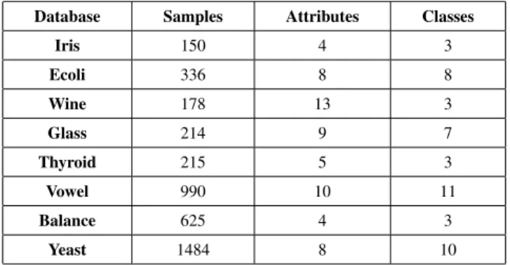
We evaluated our experiments using eight datasets of the UCI Machine Learning Repository [22] and four 2D datasets which were artificially created with the svm-toy application of the libsvm package [21]. The features of each of the UCI datasets were scaled to the interval [−1,+1] whereas those of the artificial datasets to[0,1]. The characteristics of each dataset of the UCI repository can be seen in Table I and the four artificially created datasets are illustrated in Figure 1.
TABLE I
UCI MACHINELEARNINGREPOSITORYDATASETSCHARACTERISTICS Database Samples Attributes Classes
Iris 150 4 3 Ecoli 336 8 8 Wine 178 13 3 Glass 214 9 7 Thyroid 215 5 3 Vowel 990 10 11 Balance 625 4 3 Yeast 1484 8 10
B. Default Sub-class ECOC configuration
The PSO resulting splitting parameters were compared with the set of default parameters θ={θperf,θsize,θimpr}
which were fixed in each dataset to the following values [1]: • θperf = 0%, split the classes if the classifier does not
attain zero training error.
• θsize = |50J|, minimum number of samples in each
constructed cluster, where|J|is the number of features in each dataset.
• θimpr= 5%, the improvement of the newly constructed
binary problems after splitting.
Furthermore, as a clustering method we used the K-means algorithm with the number of clusters K= 2. As stated by Escalera et al. [1], the K-means algorithm obtains similar
0.1 0.2 0.3 0.4 0.5 0.6 0.7 0.8 0.2 0.3 0.4 0.5 0.6 0.7 0.8 0.9 1
(a) Artificial dataset #1
0 0.1 0.2 0.3 0.4 0.5 0.6 0.7 0.8 0.9 0.2 0.3 0.4 0.5 0.6 0.7 0.8 0.9 1 (b) Artificial dataset #2 0 0.1 0.2 0.3 0.4 0.5 0.6 0.7 0.8 0.9 1 0.1 0.2 0.3 0.4 0.5 0.6 0.7 0.8 0.9 (c) Artificial dataset #3 0 0.1 0.2 0.3 0.4 0.5 0.6 0.7 0.8 0.9 0 0.1 0.2 0.3 0.4 0.5 0.6 0.7 0.8 0.9 1 (d) Artificial dataset #4 Fig. 1. Artificial Datasets.
results with other more sophisticated clustering algorithms, such as hierarchical and graph cut clustering, but with much less computational cost.
C. Default SVM configuration
As a standard classifier for our experiments we used the libsvm implementation of the Support Vector Machine with linear and RBF kernel. We compared our optimized classifier against the default classifier used in the libsvm package, that is a linear SVM with C= 1and an RBF SVM withC= 1
andσ= 1/attributesnr, whereattributesnr is the number
of features in each dataset. D. Results
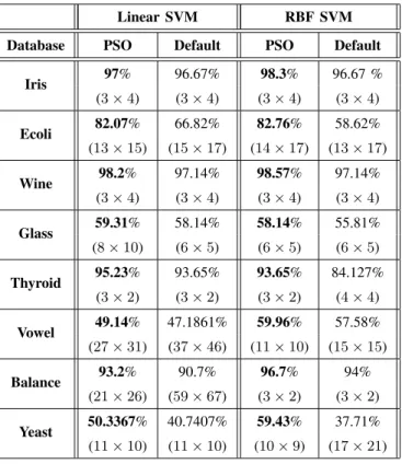
The resulting classification performances attained in our experiments are shown in Tables II and III. In the case of the sub-ECOC method we also give the (number of rows× number of columns) of the encoding matrices formed.
From the results, it is obvious that the optimized sub-ECOC using PSO always outperforms the default classifiers in all of the experiments conducted. The improvement is attributed to the fact that PSO finds the optimum values for the thresholds that control the resulting number of subclasses. Furthermore, by finding via PSO optimum values for the SVM parameters (i.e., C and σ), the classification perfor-mance is further improved. In certain datasets the thresholds returned by PSO do not result in any subclasses. In this case, PSO reveals that, in the specific dataset, it is highly probable that the use of subclasses will lead to over-fitting. We can also see that in the RBF SVM the performance improvement is more significant than in the Linear SVM. This can be
TABLE II
UCI REPOSITORYEXPERIMENTS FORLINEAR ANDRBF SVM.
Linear SVM RBF SVM
Database PSO Default PSO Default
Iris 97% 96.67% 98.3% 96.67 % (3×4) (3×4) (3×4) (3×4) Ecoli 82.07% 66.82% 82.76% 58.62% (13×15) (15×17) (14×17) (13×17) Wine 98.2% 97.14% 98.57% 97.14% (3×4) (3×4) (3×4) (3×4) Glass 59.31% 58.14% 58.14% 55.81% (8×10) (6×5) (6×5) (6×5) Thyroid 95.23% 93.65% 93.65% 84.127% (3×2) (3×2) (3×2) (4×4) Vowel 49.14% 47.1861% 59.96% 57.58% (27×31) (37×46) (11×10) (15×15) Balance 93.2% 90.7% 96.7% 94% (21×26) (59×67) (3×2) (3×2) Yeast 50.3367% 40.7407% 59.43% 37.71% (11×10) (11×10) (10×9) (17×21) TABLE III
ARTIFICIALDATASETSEXPERIMENTS FORLINEAR ANDRBF SVM.
Linear SVM RBF SVM
Database PSO Default PSO Default
Set # 1 98.68% 94.74% 100% 59.21 % (14×16) (19×23) (4×3) (3×2) Set # 2 87.72% 59.65% 82.76% 58.62% (50×58) (48×56) (14×17) (13×17) Set # 3 70.56% 64.56% 82.36% 77.89% (5×4) (3×2) (4×3) (3×2) Set # 4 52.49% 43.89% 79.86% 40.28% (113×151) (113×151) (21×25) (114×153)
associated to the major role the σ parameter plays in the classification performance of the RBF SVM.
X. CONCLUSION
ECOC with subclasses is a power classification technique that takes advantage of the fact that by splitting the classes we can create more complex discriminant surfaces. As men-tioned, the splitting is parameter dependent and there’s no standard way to choose the right values for these parameters. If the values we choose are very strict, we will create very complex surfaces that will improve the training performance of the classifier, but will probably result in over fitting in the test domain. On the other hand, if we choose very
loose values we will not take full advantage of the subclass technique. From the above, it is clear that the splitting parameters need some kind of optimization. As we showed here by applying PSO optimization we can find optimum values for the splitting parameters resulting in much better classification performance.
REFERENCES
[1] Sergio Escalera, David M.J. Tax, Oriol Pujol, Petia Radeva and Robert P.W. Duin, “Subclass Problem-Dependent Design for Error-Correcting Output Codes,”IEEE Transactions on Pattern Analysis and Machine Intelligence, vol. 30, pp. 1041–1054, June 2008.
[2] Sergio Escalera, Oriol Pujol and Petia Radeva, “Loss-Weighted Decod-ing for Error-CorrectDecod-ing Output CodDecod-ing”Proc. Int’l Conf. Computer Vision Theory and Applications, vol. 2, pp. 117–122, June 2008. [3] Oriol Pujol, Petia Radeva and Jordi Vitria, “Discriminant ECOC A
Heuristic Method for Application Dependent Design of Error Correcting Output Codes,”IEEE Transactions on Pattern Analysis and Machine Intelligence, vol. 6, pp. 1001–1007, June 2006.
[4] Vladimir Vapnik,Statistical Learning Theory, Wiley & Sons, 1998. [5] Thomas G. Dietterich and Ghulum Bakiri, “Solving Multi-class
Learn-ing Problems via Error-CorrectLearn-ing Output Codes,”Journal of Machine Learning Research, vol. 2, pp. 263–282, 1995.
[6] Erin L. Allwein, Robert E. Schapire and Yoram Singer, “Reducing Multi-class to Binary: A Unifying Approach for Margin Classifiers,” Journal of Machine Learning Research, vol. 1, pp. 113–141, 2002. [7] Kari Torkkola, “Feature Extraction by Non-Parametric Mutual
Informa-tion MaximizaInforma-tion,”Journal of Machine Learning Research, vol. 3, pp. 1415–1438, March 2003.
[8] P. Pudil, F.J. Ferri, J. Novovicova and J. Kittler, “Floating Search Meth-ods for Feature Selection with Non-monotonic Criterion Functions,” Proc. Int’l Conf. Pattern Recognition, vol. 3, pp. 279–283, March 1994. [9] J. Kapur and H. Kesavan,Entropy Optimization principles with
Appli-cations, Academic Press, 1992.
[10] E.B. Kong and T.G. Dietterich, “Error-Correcting Output Coding Corrects Bias and Variance,”Proc. 12th Intl Conf. Machine Learning pp. 313–321, 1995.
[11] Richard O. Duda and Peter E. Hart and David G. Stork, Pattern Classification,Wiley-Interscience, 2nd Edition, 2000.
[12] J. Kennedy and R.C. Eberhart, “Particle Swarm Optimization,”Proc. IEEE Int’l Joint Conf. Neural Networks, vol. 3, pp. 279–283, March 1994.
[13] R.C. Eberhart, P.K Simpson and R.W. Dobbins,Computational Intel-ligence Tools, Academic Press Professional, first edition, 1996. [14] Y.Shi and R.C. Eberhart, “A modified Particle Swarm Optimizer,”
Proc. IEEE Congress on Evolutionary Computation, vol. 3, pp. 279– 283, March 1994.
[15] F. van den Bergh, An analysis of Particle Swarm Optimizers, PhD thesis, Department of Computer Science, University of Pretoria, South Africa, 2002
[16] F. van den Bergh and A.P. Engelbrecht, “A Study of Particle Swarm Optimization Swarm Trajectories,” Information Sciences, vol. 3, pp. 937–971, March 1994.
[17] S. Naka, T. Genji, T. Yura and Y. Fukuyama, “Practical Distribution State Estimation using Hybrid Particle Swarm Optimization,” Proc. IEEE PowerEngineering Society Winter Meeting, vol. 2, pp. 815–820, 2001.
[18] A. Ratnaweera, S. Halgamuge and H. Watson, “Particle Swarm Opti-mization with Self-Adaptive Acceleration Coefficients,”Proc. First Int’l Conf. Fuzzy Systems and Knowledge Discovery, pp. 264–268, 2003. [19] P.N. Suganthan, “Particle Swarm Optimizer with Neighborhood
Op-erator,”Proc. IEEE Congress on Evolutionary Computation, pp. 1958– 1962, 1999.
[20] H. Yoshida, Y. Fukuyama, S. Takayama and Y. Nakanishi, “A Particle Swarm Optimization for reactive Power and Voltage Control in Electric Power Systems Considering Voltage Security Assessment,”Proc. IEEE Int’l Conf. Systems, Man, and Cybernetics, vol. 6, pp. 497–502, Oct. 1999.
[21] Chih-Chung Chang and Chih-Jen Lin,LIBSVM: a library for support vector machines, http://www.csie.ntu.edu.tw/ cjlin/libsvm, 2001. [22] A. Asuncion and D.J. Newman,UCI Machine Learning Repository,
University of California, Irvine, School of Information and Computer Sciences, http://www.ics.uci.edu/ mlearn/MLRepository.html, 2007.