OPEN-SET EVOLVING ACOUSTIC SCENE CLASSIFICATION SYSTEM
Fatemeh Saki, Yinyi Guo, Cheng-Yu Hung
Lae-Hoon Kim, Manyu Deshpande, Sunkuk Moon, Eunjeong Koh, and Erik Visser
Qualcomm Technologies, Inc., San Diego, USA
ABSTRACT
Most audio recognition/classification systems assume a static and closed-set model, where training and testing data are drawn from a prior distribution. However, in real-world audio recognition/classification problems, such a distribution is un-known, and training data is limited and incomplete at training time. As it is difficult to collect exhaustive training samples to train classifiers. Datasets at prediction time are evolving and the trained model must deal with an infinite number of unseen/unknown categories. Therefore, it is desired to have an open-set classifier that not only accurately classifies the known classes into their respective classes but also effectively identifies unknown samples and learns them. This paper in-troduces an open-set evolving audio classification technique, which can effectively recognize and learn unknown classes continuously in an unsupervised manner. The proposed method consists of several steps: a) recognizing sound signals and associating them with known classes while also being able to identify the unknown classes; b) detecting the hidden unknown classes among the rejected sound samples; c) learn-ing those novel detected classes and updatlearn-ing the classifier. The experimental results illustrate the effectiveness of the de-veloped approach in detecting unknown sound classes com-pared to extreme value machine (EVM) and Weibull-cali-brated SVM (W-SVM).
Index Terms—Acoustic scene classification, open-set recognition, support vector data description
1. INTRODUCTION
Research on acoustic scene classification (ASC) has been receiving increased attention over the past decade, which has led to a consid-erable amount of new sound modeling and recognition techniques. ASC plays a major role in machine hearing systems. Where, the pri-mary goal is achieving human-like auditory recognition of ambient sound signals [1, 2]. Some example applications include context-aware devices that automatically adjust their operation mode accord-ing to surroundaccord-ing sounds, such as hearaccord-ing aid devices that their speech enhancement parameters are adjusted depending on the back-ground noise type [3]. Some other applications are robotics [4], mon-itoring elderly people, and acoustic monmon-itoring systems in smart homes for detecting events such as glass breaking, baby crying, and gunshot [5].
One limitation of the existing ASC systems is their closed-set nature, that is a fixed and limited number of known classes are used during the training. In closed-set classifiers, it is assumed that during test time, the test data is drawn from the same set of classes as the training data. This guarantees that every input samples are classified into exactly one of the training classes. However, most applications for ASCs in nature are open-set problems. In other words, in an open-set framework, the test data could include samples associated with unknown classes as well. Therefore, it is necessary for an ASC to detect if a sound signal is associated with an unknown category. It is also desired to learn the unknown instances that appear more frequently. To our knowledge, the following contributions are the only existing ASC systems that partially implement the open-set framework. In [6] an open-set ASC is proposed to detect unknown classes utilizing support vector data description (SVDD). This method is only able to detect unknown samples without being able to learn them. In [7], a real-time unsupervised model for learning environmental noise signals is developed. This model can detect un-known classes in the stream of input sound signals and learn them on the fly. However, it can only store data from one unknown class and create one class at a time.
In this work, we propose a solution to overcome the limitations of both systems. Our proposed technique can identify the unknown sound signals and classify them into multiple micro-clusters based on the similarity of their characteristics. We then prune the micro-clusters according to a popularity measure, such that the micro-clus-ters larger than a certain threshold are classified into new classes on the fly. Importantly, our proposed method has no limitation on the number of classes created on the fly.
The rest of the paper is organized as follows. A brief overview of the set problem is covered in Section 2. The proposed open-set evolving acoustic scene classification model is then presented in Section 3. Section 4 presents the experimental results followed by the conclusion in Section 5.
2. OPEN-SET RECOGNITION MODEL
In this section, we first briefly state the preliminaries related to open-set recognition (OSR), following which we formally define the evolving open-set problem in Section 3.
Traditional recognition/classification algorithms are closed-set problems where all training and testing data are known a priori. Closed-set classifiers have been developed that maximize the opti-mal posterior probability, 𝑝(𝐶𝑖|𝑥; 𝐶1, 𝐶2, … 𝐶𝑀), 𝑖 ∈ {1,2, … , 𝑀},
where 𝑥 is an input sample, 𝑖 is the index of the known class 𝐶𝑖, and
𝑀 in the number of the known classes. However, a practical auto-matic recognition/classification problem is an open-set problem,
https://doi.org/10.33682/en2t-9m14
where during testing, data from unknown classes can emerge at any time unexpectedly. Therefore, during the test, the optimal posterior probability becomes 𝑝(𝐶𝑗|𝑥; 𝐶1, 𝐶2, … 𝐶𝑀, 𝐶𝑀+1, . . 𝐶𝑀+𝑄), 𝑗 ∈
{1,2, … , 𝑀 + 𝑄}, with 𝑄 being the number of unknown classes [8]. This posterior probability cannot be modeled as classes 𝐶𝑀+1
through 𝐶𝑀+𝑄 are unknown.
In [9], the OSR problem was formalized for the first time and a preliminary solution was proposed. It incorporates an open space 𝑂 risk term to account for the space beyond the reasonable support of the known classes. Open space is a space that is sufficiently far from the known classes. Let 𝑓 be a measurable function where 𝑓𝑦(𝑥) ≥ 0
implies recognition of the known class 𝑦 and 𝑓𝑦(𝑥) = 0 implies,
in-put 𝑥 does not belong to class 𝑦. The open space risk 𝑅𝑜(𝑓) for a
class 𝑦 can be defined as follows [9]: 𝑅𝑜(𝑓𝑦) =
∫ 𝑓𝑂 𝑦(𝑥)𝑑𝑥 ∫ 𝑓𝑆𝑜 𝑦(𝑥)𝑑𝑥
(1)
where 𝑆𝑜 is the space that contains all the known training classes as
well as the open space 𝑂. The objective OSR function must balance the open space risk against empirical error.
The OSR problem has been studied in various frameworks [10-12]. In [12] the existing open-set techniques are categorized into five main categories. 1) deep neural network-based, 2) adversarial learn-ing-based, 3) extreme value theory-based, 4) Dirichlet process-based, and 5) traditional machine learning-based models. Although much effort has been made to develop promising solutions for OSR prob-lem, the flexibility of these methods in continuously learning new classes, at a lower computational complexity, is still a challenge. Ad-dressing this challenge using traditional machine learning ap-proaches is the focus of this paper.
3. MULTI-CLASS OPEN-SET EVOLVING ACOUSTIC
SCENE CLASSIFICATION MECHANISM
A dynamically evolving classification system needs to continuously detect unknown classes and learn them at a low training cost. The key components of such a system are as follows: 1) accurately as-signing the input samples from the known classes into their respec-tive labels, 2) rejecting samples that are from unknown classes, 3) keeping track of the rejected unknown samples to identify potential new classes among all the rejected samples in 2), and 4) learning/la-beling the detected new classes and expanding the existing model at a low training cost.
In this work, similar to [7], known classes are labeled with pos-itive integers and unknown samples are temporarily labeled as 0. As-suming 𝑥 ∈ ℝ𝑑 to be an input sample in the feature domain, the
pro-posed open-set evolving model is defined as follows.
Definition (Multi-class Open-set Evolving Recognition (MCOSR) Model): A solution to a multi-class open-set evolving recognition:
1.A multi-class open-set model 𝐹(𝑥): ℝ𝑑↦ ℤ≥0 is an ensemble
of multiple OSR functions, 𝑓𝐶𝑖(𝑥) ∶ ℝ
𝑑↦ ℝ, 𝑖 = 1, … , 𝑀,
where 𝑀 is the number of known classes.
2.Let 𝒳𝑁𝑜𝑣≔ {𝑥𝑘|𝑥𝑘∈ ℝ𝑑, 𝑘 = 1, … , 𝒦} be a dataset of 𝒦
sam-ples, that are detected as unknown. 𝐿(𝒳𝑁𝑜𝑣): ℝ𝑑↦ ℕ is a
nov-elty detection process that is applied to 𝒳𝑁𝑜𝑣 to determine the
existence of new classes in 𝒳𝑁𝑜𝑣.
3.If 𝐿(𝒳𝑁𝑜𝑣) discovers 𝑄 potential new classes, the existing
MCOSR model is expanded by adding the discovered classes to the previously learned class set. Thus, the set of known classes becomes {𝐶1, 𝐶2, … , 𝐶𝑀} ∪ {𝐶𝑀+1, 𝐶𝑀+2, … , 𝐶𝑀+𝑄}. It is worth
noting that 𝑀 varies in time as a result of the evolution process. The diagram of the proposed MCOSR is shown in Fig. 1. Details of each step are introduced in the following subsections.
3.1. Multi-class open-set evolving recognition function
This section states the details of the proposed open-set acoustic scene classification. The algorithm consists of four main steps, fea-ture extraction, classification/rejection, new class detection, and model evolution as follows.
3.1.1. Feature extraction:
The spectrogram of the input audio signal is first passed through a pre-trained neural network (details discussed in section 4)to extract the embedding representation. In this work, an L3-Net-based [13] audio embedding network is used as the feature extractor. The ex-tracted embeddings are used as the input feature vectors to the MCOSR model.
3.1.2.Classification/rejection
The extracted embeddings from an input sound file are passed into the multi-class open-set recognition model 𝐹(𝑥): ℝ𝑑↦ ℤ≥0 to
de-termine if the input sound signal belongs to any of the known clas-ses, 𝐶𝑖, or it is an unknown sample (0). 𝐹(𝑥) is an ensemble of
mul-tiple OSR functions, 𝑓𝐶𝑖(𝑥) ∶ ℝ
𝑑↦ ℝ, 𝑖 = 1, … , 𝑀, where 𝑀 is
the number of known classes. Each of the OSR functions character-izes one of the known classes utilizing a support vector data descrip-tion (SVDD) model [14].
SVDD is a kernel-based sphere-shaped data description method that provides an effective description of the data boundary in the fea-ture space. SVDD has been investigated in the context of various open-set problems [15,16]. The objective of SVDD is to find the
smallest hypersphere that encloses most of the data in feature space 𝒳. Let 𝒳 ≔ {𝑥𝒿|𝑥𝒿∈ ℝ𝑑, 𝒿 = 1, … , 𝒥} be a dataset of 𝒥
points. Using a nonlinear transformation 𝜑 from 𝒳 to a high-dimen-sional kernel feature space, the smallest enclosing hypersphere of radius 𝑅 and center 𝛼 can be stated as:
min 𝑅,𝛼,𝜉𝑅 2+1 𝛾∑ 𝜉𝑗 𝒿 (2) 𝑠. 𝑡. ‖𝜑(𝑥𝒿) − 𝛼‖ 2 ≤ 𝑅2+ 𝜉 𝒿, 𝜉𝒿≥ 0, ∀𝒿. (3)
The slack variables 𝜉𝒿≥ 0, associated with each training sample
𝑥𝒿, allow a soft boundary and hyperparameter 𝛾 ∈ (0,1] establishes
a traoff between the sphere volume and the accuracy of data de-scription. To optimize 𝛼, 𝑅 and 𝜉𝒿 [14] a Lagrangian procedure is
used. The local maximum of the Lagrange function can be written as:
ℒ = ∑𝒥𝒿=1𝛽𝒿𝜑(𝑥𝒿). 𝜑(𝑥𝒿) −∑𝒥𝒿,𝓀 =1𝛽𝒿𝛽𝓀𝜑(𝑥𝒿). 𝜑(𝑥𝓀) (4) 𝑠. 𝑡. ∑ 𝛽𝒿 𝒿 = 1, 𝛼 = ∑ 𝛽𝒿 𝒿𝜑(𝑥𝒿) , 0 ≤ 𝛽𝒿≤ 𝛾
where 𝛽𝒿≥ 0 represent Lagrange multipliers. Samples with 𝛽𝒿= 0
lie inside the sphere surface, while those with 𝛽𝒿= 𝛾 fall outside.
Samples with 0 < 𝛽𝒿< 𝛾 are on the boundary of the corresponding
hypersphere. It can be seen from (4), the center of the sphere (𝛼) is a linear combination of the data samples. To describe the hy-persphere, only samples with 𝛽𝒿> 0 are needed, hence they are
called support vectors. 𝑅2 is the distance from the center of the
sphere (𝛼) to (any of the support vectors on) the boundary, excluding the ones outside the sphere.
Therefore, given a set of 𝒥 data samples, the open-set recognition function for representing it as a class/hypersphere 𝐶𝑖 is defined as:
𝑓𝐶𝑖(𝑥) = ‖𝜑(𝑥) − 𝛼𝑖‖ 2− 𝑅
𝑖2 (5)
Input 𝑥 is associated with class 𝐶𝑖, if its distance to the center
of the sphere 𝐶𝑖 ,i.e. 𝛼𝑖, is equal or smaller than the radius 𝑅𝑖2, i.e.
𝑓𝐶𝑖(𝑥) ≤ 0. Therefore, the decision mechanism of identifying the
la-bel of the input sample 𝑥 in MCOSR is as follows: 𝐶∗= {𝑎𝑟𝑔 min𝑖 𝑓𝐶𝑖(𝑥) 𝑓𝐶𝑖(𝑥) ≤ 0, ∀ 𝑖 = 1, … , 𝑀
0 𝑜𝑡ℎ𝑒𝑟𝑤𝑖𝑠𝑒 (6) The 𝐶∗ is the output label, where 0 stands for unknown samples.
To minimize misclassifications, majority voting of 3 decisions is considered. This way if inputs at time 𝑡 and 𝑡 + 2, 𝑥𝑡 and 𝑥𝑡+2 are
both from class ℓ, then 𝑥𝑡+1 is expected to be from the same class,
noting that signal data occur in a streaming manner and the interest is primarily on the sustained type of sound.
3.1.3.Model evolution with detected new classes
Samples that are detected as unknown are stored in a buffer. Length of this buffer should be larger than a minimum number of samples, 𝒟, required for establishing a new class. Let 𝒳𝑁𝑜𝑣≔ {𝑥𝑘|𝑥𝑘∈
ℝ𝑑, 𝑘 = 1, … , 𝒦} be the set of 𝒦 samples in the buffer. Among
these stored unknown samples, we need to determine if there is any consolidated ensemble that should be declared as a new separate class. A similarity measure is used to assess such consolidation. Let 𝐿(. ): ℝ𝑑↦ ℕ to be the process of detecting the existence of a new
class using that similarity measure. We use cosine similarity meas-ure and denote a pair of data points as similar if their cosine simi-larity is greater than a predefined threshold value 𝜆. In this work,
this value is set empirically to 𝜆 = 0.85. An ensemble of similar samples is called cluster. A sample is assigned to a micro-cluster if its similarity not only with the center of the micro-micro-cluster, but also with each sample from a randomly selected set, is greater than 𝜆. If not assigned to any of the existing micro-clusters, the sam-ple will form a sporadic micro-cluster. Micro-clusters with size less than two are considered sporadic. Once the size of a micro-cluster exceeds 𝒟, an open-set recognition function, e.g. SVDD, is used to model it as a new class. To set 𝒟, one needs to specify how long an occurring sound to be sustained in order to establish a new class. In other words, how long sound data from a scene class is needed to establish a new class. Finally, when a new class is created, the pre-trained model gets updated accordingly. The newly created class is labeled as the number of existing classes plus one.
4. EXPERIMENTAL RESULTS
In this section, we evaluate the performance of MCOSR algorithm in terms of OSR accuracy, and qualitatively analyze its evolving as-pects. We then perform a comparative study of the OSR accuracy of the proposed method against the existing state-of-the-art OSR al-gorithms such as EVM [8], Weibull-calibrated SVM (W-SVM) [17], PI-SVM and PI-OSVM (one-class SVM) [18]. EVM has a well-grounded interpretation derived from the statistical extreme value theory (EVT) and is the first classifier capable of performing nonlinear kernel-free learning. In W-SVM, the decision scores are used to fit the data into a single Weibull distribution, and a specific threshold is set to reject the unknown classes [8].
Data from the DCASE 2018 task5, a subset of SINS [19], TUT Acoustic Scenes 2017 [20], and Audioset [21] are used to evaluate the proposed algorithm. The dataset comprises 12 acoustic scenes, which are “absence”, “cooking”, “dishwashing”, “eating”, “social activity”, “watching TV”, “car”, “music”, “restaurant”, “transport”, “vacuum cleaner”, and “working”.
OpenL3 [22] is used for extracting the audio embeddings, con-sidering the default settings and a 512-embedding dimension. The input to the L3-Net is a 10-second audio signal and the extracted embedding feature is a matrix of size 96×512. The averages of the extracted embeddings from the 10-second sound files are used as inputs to the MCOSR.
We begin by pre-training a model using data from the follow-ing five acoustic scenes “cookfollow-ing”, “dishwashfollow-ing”, “eatfollow-ing”, “social activity”, and “watching TV”. This leads to five pre-trained classes, which we will refer to as C1, C2, …, C5, respectively. For pre-train-ing, we used 30 audio embedding samples, i.e. 𝒟, extracted from five minutes of sound signals per acoustic scene. The remaining du-ration of data associated with the five pre-training scenes, men-tioned above, along with the full duration of the data associated with the other seven acoustic scenes, i.e. “absence”, “car”, “music”, “res-taurant”, “transport”, “vacuum cleaner”, and “working”, are used for testing.
4.1. Multi-class open-set recognition
We evaluate the OSR aspect of the MCOSR in two steps. In the first step, the proposed system identifies if an input sample is associated with the pre-trained classes and if so, it labels them as known sam-ples. In the second step, the system classifies the known samples into their respective classes, which is known as closed-set recogni-tion. Denote by 𝑇𝑃, 𝐹𝑃, 𝑇𝑁, and 𝐹𝑁 the true-positive, false-posi-tive, true-negative and false-negafalse-posi-tive, respectively. We measure the
accuracy of the first step in the form of true-positive rate, given by 𝑇𝑃𝑅 = 𝑇𝑃/(𝑇𝑃 + 𝐹𝑁), and specificity, that is 1 − 𝐹𝑃𝑅 = 𝑇𝑁/ (𝑇𝑁 + 𝐹𝑃). The results are reported in Table 1, where each entry is an average of a 10-fold cross-validation process.
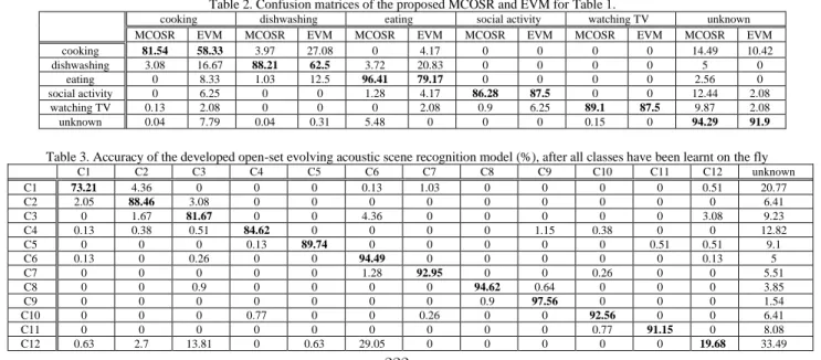
Aside from MCOSR results, Table 1 also reports the results for comparable algorithms in the literature, including EVM, W-SVM, PI-SVM, and PI-OSVM. The rejection threshold, i.e. 𝛿, for EVM is set to 0.05, which is deduced empirically. At first glance, it may appear that W-SVM outperforms other algorithms since its specific-ity is slightly higher than that of MCOSR and EVM. However, it drastically underperforms, in terms of 𝑇𝑃𝑅, compared to MCOSR and EVM. It is worth mentioning that, EVM has the highest 𝑇𝑃𝑅 while its specificity is close to the MCOSR. Importantly, as reported in Table 2, EVM suffers from large confusion error in close-set recognition. Our analyses suggest that PI-OSVM and PI-SVM pro-vide the lowest performance.
4.2. The performance of the open-set technique as a function of class-set evolution
In this section, we study the performance of our proposed algorithm while changing the order in which the data are fed to the system. Our contribution is two-fold. First, we investigate the effect of choosing the initial sound samples on the number of created classes during the test and their accuracy. Next, we measure the overall post-evolution accuracy of the system, in terms of a confusion ma-trix.
To evaluate the effect of the initial sound samples on the per-formance of the proposed MCOSR technique, we used a pre-trained model comprising C1, C2, C3, C4, and C5. During the test, the in-puts to the pre-trained model are the samples from known and un-known classes. The experiment is repeated 10 times while randomly
shuffling the sound files associated with each class. Samples that are detected as unknown are stored in a buffer. The 𝐿(. ) process is continuously assessing the existence of a new class among the stored unknown samples. Once it detects a new class, MCOSR to be updated with this new class and the set of known classes is ex-panded. It is expected the forthcoming samples from the newly added class to be assigned to it and not identified as unknown sam-ples anymore. However, in some of the experiments, MCOSR cre-ates multiple classes for “music” class. Because the music data is not coherent enough, the initially created music class by MCOSR does not provide enough representative information of the music class. Therefore, other incoming music samples are identified as un-known samples and later will be learned as a new class. Data from the “working” sound scene is also a challenging one. In some ex-periments, no new class is created for this scene, as data from this scene is always misclassified by one of the known classes, mostly the “absence” class. Also, the samples from this scene that are iden-tified as unknown are not similar enough to create meaningful mi-cro-clusters to be declared as a new class.
As mentioned earlier, we next measured the post-evolution ac-curacy of the system. The results are reported in Table 3 in terms of a confusion matrix. In this table “absence”, “car”, “music”, “restau-rant”, “transport”, “vacuum cleaner”, and “working” scenes are re-ferred as C6, C7, …, C12, respectively. It was found as the number of classes increases in the model; the confusion rate increases. Be-cause SVDD ignores the discriminative information between the known classes, which leads to poor classification performance. This issue needs to be addressed to achieve a higher classification accu-racy when dealing with more complex acoustic scenes.
5. CONCLUSION
This paper provides an open-set evolving audio scene classification technique, MCOSR, which can effectively recognize and learn un-known acoustic scenes in an unsupervised manner. The developed model is evaluated utilizing the DCASE challenge dataset, TUT Acoustic Scenes 2017, and music files from Audioset. Experimental results demonstrate the effectiveness of the developed approach in identifying unknown samples compared to EVM, W-SVM, PI-OSVM, and PI-SVM. This paper exemplifies how the proposed MCOSR method can be used as a proper evolving open-set system for sound classification applications. Future research will focus on addressing practical issues during run time.
Table 2. Confusion matrices of the proposed MCOSR and EVM for Table 1.
cooking dishwashing eating social activity watching TV unknown
MCOSR EVM MCOSR EVM MCOSR EVM MCOSR EVM MCOSR EVM MCOSR EVM
cooking 81.54 58.33 3.97 27.08 0 4.17 0 0 0 0 14.49 10.42 dishwashing 3.08 16.67 88.21 62.5 3.72 20.83 0 0 0 0 5 0 eating 0 8.33 1.03 12.5 96.41 79.17 0 0 0 0 2.56 0 social activity 0 6.25 0 0 1.28 4.17 86.28 87.5 0 0 12.44 2.08 watching TV 0.13 2.08 0 0 0 2.08 0.9 6.25 89.1 87.5 9.87 2.08 unknown 0.04 7.79 0.04 0.31 5.48 0 0 0 0.15 0 94.29 91.9
Table 3. Accuracy of the developed open-set evolving acoustic scene recognition model (%), after all classes have been learnt on the fly
C1 C2 C3 C4 C5 C6 C7 C8 C9 C10 C11 C12 unknown C1 73.21 4.36 0 0 0 0.13 1.03 0 0 0 0 0.51 20.77 C2 2.05 88.46 3.08 0 0 0 0 0 0 0 0 0 6.41 C3 0 1.67 81.67 0 0 4.36 0 0 0 0 0 3.08 9.23 C4 0.13 0.38 0.51 84.62 0 0 0 0 1.15 0.38 0 0 12.82 C5 0 0 0 0.13 89.74 0 0 0 0 0 0.51 0.51 9.1 C6 0.13 0 0.26 0 0 94.49 0 0 0 0 0 0.13 5 C7 0 0 0 0 0 1.28 92.95 0 0 0.26 0 0 5.51 C8 0 0 0.9 0 0 0 0 94.62 0.64 0 0 0 3.85 C9 0 0 0 0 0 0 0 0.9 97.56 0 0 0 1.54
Table 1. Accuracy of MCOSR, EVM, W-SVM(Linear), PI-OSVM, and PI-SVM in detecting the known classes and reject-ing the unknown classes (%), in terms of TPR (higher, better) and 1-FPR (higher, better)
Methods Detecting known:
TPR Rejecting unknown: 1-FPR MCOSR 88.22 93.03 W-SVM (Linear) 59.58 96.61 EVM 97.08 91.9 PI-OSVM 21.7 15.68 PI-SVM 60.8 51.41
6. REFERENCES
[1] S. McAdams, “Recognition of sound sources and events,” in Thinking in Sound,: the Cognitive Psychology of Human Audi-tion. London: Oxford Univ. Press, 1993.
[2] A. S. Bregman. Auditory Scene Analysis: The Perceptual Or-ganization of Sound. Cambridge, MA, USA: MIT Press, 1990. [3] I. Panahi, N. Kehtarnavaz, and L. Thibodeau,
“Smartphone-based noise adaptive speech enhancement for hearing aid appli-cations,” Proceedings of the 38th Annual International
Confer-ence of the IEEE Engineering in Medicine and Biology Society (EMBC), pp. 85-88, Orlando, August 2016.
[4] S. Aziz , M. Awais, T. Akram, U. Khan, M. Alhussein, and K. Aurangzeb, “Automatic scene recognition through acoustic classification for behavioral robotics,” Electronics 2019, vol. 8, no.5, 483.
[5] T .Virtanen, M. D. Plumbley, and D. Ellis. “Introduction to sound scene and event analysis,” Computational Analysis of Sound Scenes and Events, pp. 3-12, Springer, Cham, 2018. [6] D. Battaglino, L. Lepauloux, and N. Evans, “The open-set
problem in acoustic scene classification,” International Work-shop on Acoustic Signal Enhancement (IWAENC), pp. 1-5, 2016.
[7] F. Saki, N. Kehtarnavaz “Real-time unsupervised classification of environmental noise signals,” IEEE/ACM Transactions on Audio, Speech, and Language Processing, pp. 1657-1567, 2017.
[8] E. M. Rudd, L. P. Jain, W. J. Scheirer, and T. E. Boult, “The extreme value machine,” IEEE Transactions on Pattern Analy-sis and Machine Intelligence, vol. 40, no. 3, pp. 762-768, Mar. 2018.
[9] W. J. Scheirer, A. de Rezende Rocha, A. Sapkota, and T. E. Boult, “Toward open set recognition,” IEEE Transactions on Pattern Analysis and Machine Intelligence, vol. 35, no. 7, pp. 1757-1772, Jul. 2013.
[10]P. Phillips, P. Grother, and R. Micheals, “Evaluation methods on face recognition,” Handbook of Face Recognition, A. Jain and S. Li, eds., pp. 329-348, Springer, 2005.
[11]L. Fayin and H. Wechsler, “Open set face recognition using transduction,” IEEE Transactions on Pattern Analysis and Ma-chine Intelligence, vol. 27, no. 11, pp. 1686-1697, Nov. 2005. [12]Ch. Geng, Sh. Huang, and S. Chen, “Recent advances in open
set recognition: a survey,” http://arxiv.org/abs/1811.08581. [13]R. Arandjelovi´c and A. Zisserman, “Look, listen and learn,”
Proceedings of the IEEE International Conference on Com-puter Vision (ICCV), pp. 609–617, 2017.
[14]D. M. Tax and R. P. Duin, “Support vector data description,”
Machine learning, vol. 54, no. 1, pp. 45-66, 2004.
[15]A. Banerjee, P. Burlina, and C. Diehl. “A support vector method for anomaly detection in hyperspectral imagery,” IEEE Transactions on Geoscience and Remote Sensing, vol. 44, no. 8, pp. 2282-2291, 2006.
[16]F. Alegre, A. Amehraye, and N. Evans. “A one-class classifi-cation approach to generalised speaker verificlassifi-cation spoofing countermeasures using local binary patterns,” In Proceedings of the IEEE Sixth International Conference on Biometrics: The-ory, Applications and Systems (BTAS), pp. 1-8, 2013. [17]W. J. Scheirer, L. P. Jain, and T. E. Boult, “Probability models
for open set recognition,” IEEE Transactions on Pattern Anal-ysis and Machine Intelligence, vol. 36, no. 11, pp. 2317-2324, 2014.
[18]L. P. Jain, W. J. Scheirer, and T. E. Boult, “Multi-class open set recognition using probability of inclusion,” European Confer-ence on Computer Vision, pp. 393–409, Springer, Cham, 2014. [19]G. Dekkers, S. Lauwereins, B. Thoen, M. W. Adhana, H. Brouckxon, T. van Waterschoot, B. Vanrumste, M. Verhelst, and P. a. Karsmakers, “The SINS database for detection of daily activities in a home environment using an acoustic sensor net-work,” Proceedings of the Detection and Classification of Acoustic Scenes and Events 2017 Workshop (DCASE2017), November 2017.
[20]A. Mesaros, T. Heittola, and T. Virtanen. TUT database for acoustic scene classification and sound event detection. In 24th
European Signal Processing Conference, pp.1128-1132, Buda-pest, Hungary, 2016.
[21]J. F. Gemmeke, D. P. W. Ellis, D. Freedman, A. Jansen, W. Lawrence, R. C. Moore, M. Plakal, and M. Ritter, “Audio Set: An ontology and human-labeled dataset for audio events,” Pro-ceedings of the EEE International Conference on Acoustics, Speech and Signal Processing (ICASSP), pp.776-780,2017.
[22]J. Cramer, H. Wu, J. Salamon, and J. Pablo Bello “Look, listen and learn more: design choices for deep audio embeddings,”
Proceedings of the IEEE International Conference on Acous-tics, Speech and Signal Processing (ICASSP), pp. 3852–3856, Brighton, UK, May 2019.