Ann Arbor, MI 48109-1220
January 23, 2002
(first complete version)
Abstract
This paper offers a noncooperative behaviourally-founded solution of the complete information bargaining problem where two impatient individuals wish to divide a unit pie. We formulate the game in continuous time, with unrestricted timing and content of offers. Reprising experimental work from 1960, we introduce and exploreaspirational equilibrium — a Markovian refine-ment of subgame perfection where behaviour is governed by aspiration values (expected payoffs). The analysis is tractable, and generates many intuitive aspects of bargaining absent from the standard temporal monopoly paradigm. We find that discounted aspiration values form a martingale, and thereby compute bounds on the expected bargaining duration. We also deduce some simple implications about consecutive offers, and relate delay times, offers, and acceptance rates. Finally, we draw into question a traditional comparative static: Ceteris paribus, more impatient players can expect more of the pie.
∗We acknowledge feedback from the
seminars at Ohio State, Cornell, UPenn, Stanford, and Yale. Specifically, we thank Ted O’Donoghue and David Pearce for helpful comments. Ariel Rubinstein provided critical developmental feedback on a seed paper Lones acknowledges the ongoing support of the NSF.
†Email: [email protected]; web: ‡Email: [email protected]; web:
1
Introduction
“The whole creation groans and yearns, desiderating a principle of arbitration . . . ” — Edgeworth, Mathematical Psychics (1881), part II, page 46
The classic bargaining problem presents two individuals with the opportunity to share a dollar if they can first agree on a partition. The rebirth of interest in this subject from a modern noncooperative approach dates to Rubinstein (1982), itself related to St˚ahl (1972). He proposes a discrete time alternating offer model with payoff discounting.
We shall focus on three critical “realistic” elements of the above bargaining problem: (i) two risk neutral players 1,2 must divide a unit pie, by concurring on a feasible split; (ii) an agreement means a proposal by one player and an immediate acceptance by the other; (iii) the force for timely resolution is the players’ impatience. Like Rubinstein (1982), we shall ignore the additional (and important) element of incomplete information. Harsanyi (1956) observed: “As is well-known, ordinary economic theory is unable to predict the terms on which agreements tend to be reached in cases of . . . bilateral monopoly. Only on the basis of additionalassumptions does the theory of games furnish a determinate solution.” Rubinstein’s assumptions about the action space converted the intractable bilateral monopoly into a simple sequence of temporal monopolies: In his alternating offer bargaining model, players in turn are given the power to ask the other party to accept an offer, or to burn some of the pie by declining. This yielded a unique subgame perfect equilibrium (SPE) with an immediate agreement favouring the proposer. Temporal monopoly captures situations where the time cost of each negotiation round plays a central role in the players’ minds. While there are many situations with this critical feature, this effect intuitively should play no role in procedure-less settings. Players may well care about delay, and yet consider the reply time unimportant for this delay.
This paper explores the bargaining problem without temporal monopoly, and instead aims for a behaviourally motivated noncooperative solution. Since discrete time forces temporal monopoly, we shift to continuous time, where there are infinitely many SPE. View a discrete time model, or more generally temporal monopoly, as a restriction of the feasible action space to a subset of continuous time. We instead build the behavioural foundation into the solution concept — aspirational equilibrium (AE). In this Markovian refinement of SPE, players’ behaviour is governed by their aspiration values, or expected payoffs in the game. While quite tractable as we will see, the resulting theory is richer than temporal monopoly, and offers many compelling new economic insights into bargaining.
Continuous Time Bargaining and Aspirational Equilibrium. As argued, to avoid the temporal monopoly outcome, we must allow players to react instantaneously, and thereby must start with a model nested from the outset in continuous time. Continuous time models introduce a host of well-known problems, most especially the twin issues that (i) outcome profiles need not be well-defined given strategies, and (ii) best replies need not exist. We construct an extensive form game that eludes both problems. This extensive form game uses the novel idea of a two-dimensional vector time and a restriction on histories that precludes the players from conditioning their actions on time. We succinctly
summarize this feature of our extensive form as sealed-envelope instructions — at offer decision nodes, the players simultaneously commit to mixed (offer, time) pairs.
With this new structure, outcome profiles are well-defined, and we introduce four assumptions that refine SPE. The first three essentially ensure time stationary strategies, disallowing time-dependent offers, or bargaining as cheap talk or protocol. The fourth assumption asks that strategies coincide after any histories with the same expected payoffs.
The Intuitive Structure of Aspirational Equilibria. For a flavour of this refinement, consider an AE without immediate agreement. As strategies depend on expected payoffs alone and not on time, delay owes solely to the players’ randomization. With strict time preference, there are rents from ending this bargaining hiatus. And since any player is indifferent about proposing, only the opponent strictly benefits from this offer. In other words, any delay implies that the players are locked in a war of attrition: Each strictly prefers that his counterpart and not himself stop the clock and propose. To summarize, an endogenous‘proposee’ advantage arises, since receiving an offer makes one better off. This is precisely opposite to the hard-wired proposer advantage with temporal monopoly, and is the ultimate source of the different implications between these bargaining paradigms.
Next consider what transpires when some player, say Mr. 1, finally tenders an offer to Mr. 2. The latter might accept it with probability one. If so, game over. Assume not. Agreement brings us to the Pareto frontier, and is efficient, while rejection incurs further delay, and is inefficient. Since Mr. 2 weakly prefers to reject, Mr. 1 must be disappointed by this outcome, suffering a strict payoff loss if Mr. 2 declines, and payoff jump otherwise. This yields several desirable and realistic bargaining features: (i) wars of attrition explain negotiation lags; (ii) serious offers are concessions; (iii) offers may be turned down; (iv) proposers are strictly disappointed from rejection, and strictly pleased by acceptance.
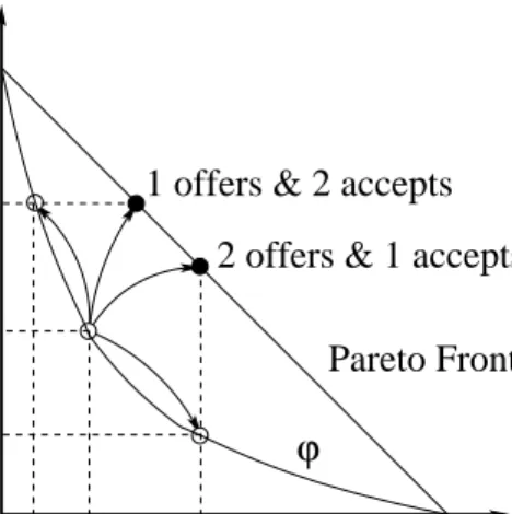
An AE specifies exogenously-given aspiration levels for the players — the initial state of a Markov process. Once Mr. 1 offers x, Mr. 2’s aspiration value jumps to this new level x. Afterwards, the concession that is offered may yet be rejected. (See Figure 1.) This leads to a tractable Markov and martingale stochastic process on the space of possible pairs of discounted aspiration levels (Theorem 4). We can then conclude that bargaining almost surely ends in finite time; we also use this process to provide a simple lower bound on the duration of bargaining based upon observed alternating offers (Corollaries 3–4).
Contrast with Temporal Monopoly. Temporal monopoly in no way precludes en-dogenous timing — as Perry and Reny (1993), Sakovics (1993), and Stahl (1993) have clearly demonstrated. They posit continuous time bargaining games where players have tiny ‘waiting’ and ‘reaction’ times after offers. This temporal monopoly setting yields very small monopoly rents, and an accordingly small proposer advantage. Consequently, the normative predictions of our model do not obtain — wars of attrition and strict con-cessions. Since their results intuitively obtain for random but boundedly positive mean waiting times after offers, at first blush one might presume that our AE are merely special cases. But our timing is truly unrestricted — and to the player with an aspiration level approaching its highest level, offers must be tendered arbitrarily quickly (Theorem 3).
We explore some key links between when and what to offer, and what to accept. The second of consecutive offers by a player is more generous (Corollary 5). Also, incentive
constraints force a trade-off between the offer content and delay time (Corollary 6), as well as the chance an offer is rejected and the surplus it concedes (Corollary 7). We show how some properties — sweetening an offer raises its acceptance chance (Corollary 8), for one — turn on a decreasing or convex aspiration set, which we also characterize (Lemma 8–9). The distinction between a proposer and proposee advantage yields an enlightening contrast between the models. In our final result, we explore what happens if player 1 becomes more impatient. In the temporal monopoly framework, this increases player 2’s temporal advantage, and forces both players to propose pie splits more favourable to player 2. In our aspirational framework, notwithstanding the multitude of equilibria, we believe that there is insight gained from posing this question. At the very least, it questions the validity of the conclusion in the temporal monopoly world. In a word, we ask what happens to the whole equilibrium set. We argue that there is a natural bijection between AE in the two worlds where player 1 is more and less impatient. Provided player 2 offers more rapidly, all incentive conditions are restored at the current aspiration levels. With this mapping, we can see that the final outcome splits in the AE with a more impatient player 1 place player 2 more often in the strategically disadvantageous offering role. We show in Theorem 5 that this raises the expected ultimate pie share of player 1.
Experimental Support for Aspirational Approach. The salience of aspirations in decision-making has long been established in the psychology literature (Siegel 1957). In fact, its significance in bargaining has long ago been investigated in laboratory tests. Siegel and Fouraker (1960) studied a simple buyer-seller bargaining game. The project’s goal was to investigate the role of differential information on the bargaining split, seeing whether the better-informed party excelled. But among the “interesting implications”, they conclude that “the basis of both the bargainer’s ‘expectancy’ and, at least partially, of his ‘bargaining strength’ may very well be his level of aspiration” (p. 60). While the authors expected the 50-50 equal split under complete information, their experiments showed how aspirations acted as a dynamic anchor on the bids made, and explored how the exchange of offers affected these aspirations. A key role played by offers in an AE — to ratchet up the opponent’s aspiration level — was observed in a specific experiment (pp. 80–81), as was the intertemporal non-monotonicity of a player’s offer (pp. 77–90).
Relative to the literature, we take some liberty in our use of the term “aspiration.” We take Siegel and Fouraker’s phrase ‘expectancy’ literally, as our aspiration is a rational expectation and not a purely arbitrary benchmark or “reference point” against which gains and losses are compared (Gilboa and Schmeidler (1994)). For we wish to provide a non ad hoc basis for the aspirations discussed by the psychological studies. This gives the desired dynamic anchor for behavior sought by Siegel and Fouraker. A few papers (recently, Karandikar, Mookherjee, and Ray (1998)) have studied models where aspirations evolve over time. With our rational aspirations, the evolution is endogenous to the model.
Outline. Section 2 develops an extensive form with which we may formally speak of subgame perfect equilibria. This is essential, for in section 3, we develop our aspirational refinement of subgame perfection. Some immediate properties are explored in section 4, and sensitivity analysis is performed in section 5. The conclusion in section 6 links some of the details of our approach to the literature. We appendicize two technical proofs.
2
The Continuous Time Bargaining Model
A. Overview. Two players i ∈ {1,2} (often denoted i, j) must split a unit pie. The players are impatient, discounting future payoffs by possibly different positive interest rates r1, r2 >0. The players’ outside options are each zero. All parameters are common
knowledge. Bargaining transpires in real time on [0,∞). At a time of his choosing, either party may propose a pie split. Proposals must lie on the Pareto frontier where pie shares sum to one — and so may be summarized by the share x ∈ [0,1] offered to the other party. To capture the irreversibility of tendering an offer and the risk of rejecting, offers are assumed final and ‘exploding’: They must be immediately either accepted — thereby ending the game — or rejected, with no explicit future commitment. (On the other hand, we shall see that in equilibrium, rejected offers will have implied future repurcussions.)
We now formally introduce the model and the notion of subgame perfection. In so doing, there are two main problems we must tackle. First, is the possibility of simultaneous offers and immediate counteroffers. For this, we introduce a notion of vector time, thereby nuancing between the simultaneous and the instantaneous. Second, and more delicate, the existence of a well-defined outcome pathhσ from a given strategy profileσ is problematic.
For since the continuum is not well-ordered (there is no first time before or after a given moment), there need not be an initial historical cause for any current action profile.1
To handle this problem, we develop a richer notion of an action space, and maintain a standard extensive form.2 In our approach every outcome path of the extensive form is
countably discrete. This concept will better reflect the fact that a strategy must be aplan of action. That is, it must dictate what happens now given the past history.
B. Real Time Bargaining. Let S = [0,1]∪ {Y, N} be the set of the available actions when players ‘speak’, wherex∈[0,1] is the share of the unit pie offeredto the other player, and the response is Y = ‘yes’ or N = ‘no’. The vector time domain is T = [0,∞)×N. For any (t, k) ∈ T, t refers to the real time, and k refers to the artificial time at any real moment t. That is, the second componentk counts the number of events that occur at a moment in time, and increments whenever players reply instantaneously, thereby ‘stopping the clock’.3 Let  denote the natural strict lexicographic order on T, namely,
(t, k)Â(t0, k0) if t > t0 ort=t0 and k > k0. Let º be the corresponding weak order.
Apath is a countable subseth⊂ {1,2} ×S× T satisfying the following. Each element (i, s,(t, k)) ∈ h is an event, where i is the player acting, s the action taken, and (t, k) the time. If (i, s,(t, k)),(i0, s0,(t0, k0)) ∈ h then (t, k) 6= (t0, k0). If (i, s,(t, k)) ∈ h and
k > 1, then there are k −1 preceding events at time t in h, namely (i`, s`,(t, `)) ∈ h,
1For instance, Bergin and MacLeod (1993) give an example of a continuum of outcome paths that are
allconsistent with a strategy profile, but not actually determined (or caused) by that profile.
2An alternative format employed by Bergin and MacLeod (1993) allows players to condition on the
event history as well as the real time, thus formally producing a continuum of decision nodes. To tame the strategies, they introduce ‘inertia’ into the strategies. By contrast, Simon and Stinchcombe (1989) deliberately take the view of continuous time as very fine discrete time.
3We have been unable to find this approach elsewhere in the literature. An unrelated notion that also
tries to deal with the inadequacies of the real time domain owes to Fudenberg and Tirole (1985). They introduce variable intensity atoms to handle entry in pre-emption games.
`= 1, . . . , k−1; further,s` ∈[0,1] for each odd`,s` =N for each even`, and i2j−1 6=i2j.
If h contains an infinite sequence of events at real time t, then the first event after t (if one exists) must be an offer. Let P denote the set of paths.
C. Histories. For paths h ∈ P, define T1(h) = sup{t | (i, s,(t, k)) ∈ h} and T2(h) =
sup{k | (i, s,(t, k)) ∈h and t =T1(h)}. A history is a path that ends in some finite real
time, and thereby belongs toH={h ∈ P |T1(h)<∞}. A historyh∈ Hhas alast event
if there exists an element (i, s,(t, k)) ∈ h where (t, k) = (T1(h), T2(h)). We distinguish
histories with ‘last events’ from those without one.
We partition H into five sets. First, histories inHi have a standing offer by player i:
Hi ={h∈ H |(i, s,(T1(h), T2(h))) ∈h and T2(h)<∞is odd}.
By definition, when T2(h)<∞ is odd, the last event (i, s,(T1(h), T2(h))) corresponds to
an offer; i.e., s ∈[0,1]. Similarly, when T2(h)<∞ is even, the last event corresponds to
a response s∈ {Y, N}. The set of all histories where the last offer has just been accepted is HY. Similarly, HN consists of the null history and all histories ending in a rejected
offer. Finally,H \ {H1∪ H2∪ HY ∪ HN} are all other histories with no last event. There
are two types of such histories. First, histories h ∈ H+ have a cluster point, ending in
a sequence of events {(in, sn,(tn, kn)), n ∈ N}, where tn ↑ T1(h) < ∞. Second, histories
h ∈ H++ ‘end’ in a deadlock at real time T1(h) if they have the property T2(h) = ∞:
there is a sequence of events {(in, sn,(T1(h), n)), n∈N}, with sn=N for all n even.
A finite history uniquely identifies a decision node in the game tree. Here we also in-troduce an offer node “after” infinite histories associated with cluster points or deadlocks.
D. Actions and Sealed Envelope Instructions. As usual, a strategy profile σ = (σ1, σ2) will map from H into an action set. We imagine that at each decision node, a
player is called upon either to approve a tabled offer, or to submit his instructions (in an envelope to his bargaining agent) about when and what he will offer next. The action set Ai(h) of player i at h described below reflects the facts that: (a) he cannot speak if
he has just tendered an offer, or if the game has ended; (b) he must reply if an offer has just been tendered to him; (c) once an offer has been rejected, he must plan to propose an offerx∈[0,1] after some elapse time in [0,∞], possibly immediately or never (zero or infinite elapse time); but (d) it is not feasible to propose an offer at the current moment (zero elapse time) after a deadlock, where there has been no last event. Altogether,
Ai(h) = ∅ if h ∈ Hi∪ HY {Y, N} if h ∈ Hj [0,1]×[0,∞] if h ∈ HN ∪ H+ [0,1]×(0,∞] ifh ∈ H++.
We call histories h ∈ Hj reply nodes, and histories h ∈ HN ∪ H+∪ H++ offer nodes.
A strategy is a map σ onH such thatσi(h)∈Ai(h) for all h∈ H.
Hereafter, B(X) are the Borel measurable subsets of X (where the topology will be understood from the context), and ∆(X) the set of probability measures on (X,B(X)). A behaviour strategy σ is a profile of mixtures σi(h)∈∆(Ai(h)) for all histories h∈ H.
E. Histories Generated from Strategies. We now define the outcome path hσ ∈ P
generated by a strategy profile σ. A naive method to construct h(σ) is to start with the null history, and then (possibly forever) sequentially append the ‘next event’ associated with σ(h) to the current history h. However, this may not be possible because it will never advance the real time past any deadlock or cluster point.
For any (t, k),(τ, `) ∈ T, define (t, k)⊕ (τ, `) = (t +τ, `) if τ > 0 and otherwise (t, k)⊕(0, `) = (t, k+`). For short, we write (t, k)⊕τ instead of (t, k)⊕(τ,1). For any pathh∈ P, we define asuccessor path ψσ(h) determined fromhby the strategy profile σ.
There are three cases:
• Ifh∈ Hj then ψσ(h) =h∪ {(i, σi(h),(T1(h), T2(h) + 1))}
• Ifh∈ HY or T1(h) =∞ then ψσ(h) =h
• Assume h ∈ HN ∪ H+ and (xi, ti) = σi(h). If t1 = t2 = ∞, then ψσ(h) = h.
Otherwise,ψσ(h) =h∪ {(i, xi, T(h)⊕ti)}, wherei= 1 ift2 ≥t1 andi= 2 ift2 < t1.
In the first case, there’s a standing offer by j ∈ {1,2}, and i must respond at once. In the second case, the game has ended or bargaining lasts forever, since for any real time, there is always a next offer. The third case may be hardest to digest. It considers two possibilities with no offer on the table. First, both players may decide never to speak again. Alternatively, one or more players may plan to propose in finite time; if the offer is immediate, then only the artificial time advances. As an arbitrary tie-breaking rule, if both players speak simultaneously, we assume that only player 1 is heard.
For any h∈ P and (t, k)∈[0,∞)× {1, . . . ,∞}, leth(t,k) ={(i, s,(τ, `))∈h|(τ, `)¹
(t, k)}. Observe that h(t,k) = ∅ if h contains no events weakly before (t, k). Fix a pure
strategyσ. An arbitrary pathh∈ P may be inconsistent withσ as it may contain events that are not generated by σ. For example, it may be that σ(∅) = ((x1,10),(x2,20)), so
that the offer by player 1 will arrive first. Then, any history h containing events before time 10 is incompatible withσ. Accordingly, let us define
H(σ) ={h∈ P |ψσ(h(t,k))⊂h ∀(t, k)≺T(h)}.
The appendix proves that our extensive form results in a well-defined outcome profile:
Lemma 1 (Outcome Profiles) The outcome path hσ is well-defined by hσ = inf{h ∈
H(σ)|h=ψσ(h)}, where the infimum is taken w.r.t. set inclusion (hσ=∅ if H(σ) =∅).
F. Payoffs and Subgame Perfection. The payoff to a pure strategy profile σ with
hσ ∈ H
Y is the vectorπ(σ) = (π1(σ), π2(σ)), whereπi(σ) =e−rit(1−x) andπj(σ) =e−rjtx
if player i made the final offer x at time t = T1(hσ) < ∞ and player j accepted it.
Otherwise, if bargaining lasts forever, or no proposal occurs after some rejection, then
π(σ) = 0. The payoff π(σ) of a behavior strategy σ is defined by taking expectations. A behavior strategy profile σ is a subgame perfect equilibrium (SPE) if for all h ∈ H \(Hi∪ HY), any (s, t) ∈ supp(σi(h)) is a best reply to σj at h. This paper is in fact
2 offers & 1 accepts Pareto Frontier 1 offers & 2 accepts
ϕ ρ v x 1 1 x v1 ρ21 1 12 2 2
Figure 1: Example Aspiration Set, Payoff Frontier, and Transitions. Aspiration value pairs are denoted by◦, and agreements by•. Lines indicate continuations following proposals. Proposals are sometimes turned down by his opponent who is indifferent. entirely focused on a Markovian class of subgame perfect equilibria. To step back from the abstraction and fix ideas, we now give a simple example that we later revisit.
Example (Constant Acceptance Rate): In the example SPE, whenever one player’s aspiration value (his expected payoff) is vi, the other’s will be ϕ(vi), where ϕ:
(0,1) → (0,1) is the strictly decreasing function ϕ(vi) = (1−vi)/(1 + vi). Note that
ϕ=ϕ−1 and so the graph G(ϕ) is symmetric, and that v+ϕ(v)<1 for all v ∈(0,1).
Our mixed strategy equilibrium is Markovian with state space G(ϕ), and an arbitrary initial state in G(ϕ). At any v ∈ G(ϕ), each player i chooses a proposal ¯xi(v) and
randomly chooses an elapse time from an exponential distribution with parameter λi(v).
If player 1’s offer x1 prevails, say, where possibly x1 6= ¯x1(v) (if player 1 deviates), then
player 2 accepts it with fixed probabilityα∈(0,1) if x1 ≥x¯1(v), and rejects it otherwise.
If the offer is rejected, the state moves to (ϕ(x1), x1) ifx1 ≥v2, and remains atvotherwise.
The functions λj and ¯xj (j = 1,2) satisfy vi = (1−α)ϕ(¯xi(v)) +α(1−x¯i(v)). Hence,
player i is indifferent about making the (equilibrium) offer ¯xi(v) or not, and
vi = Z ∞ 0 λj(v)e−[λj(v)+ri]tx¯j(v)dt = λj(v) λj(v) +ri ¯ xj(v), (1)
so that playeriis indifferent about proposing at any moment or waiting for his opponent to propose instead. It is easy to check thatvi <(1−α)ϕ(¯xi(v))+α(1−x¯i(v)) whenxi >x¯i(v);
thus, playeri does not want to make a disequilibrium offer. Notice that since ¯xi(v)> vj,
the equilibrium offer is acceptable. Also, λi(v) <∞ everywhere; thus, deadlocks almost
surely do not occur. This also will be a general property of our aspirational equilibria. Between offer events, the players engage in a waiting game to see who will make the next offer. Eventually, one player breaks down and proposes a pie split; that offer may be rejected. The bargaining state randomly transitions through G(ϕ) as offers are made and rejected until absorption on the Pareto frontier, when an offer is finally accepted.
3
The Aspirational Refinement
Any pie split at any time is an SPE of our continuous-time model. We now introduce an equilibrium refinement motivated by the earlier psychological study of Siegel and Fouraker (1960). We assume that players’ bargaining aspirations govern their behaviour. We proceed via assumptions that ensure time-constant strategies and stationarity in payoffs.
3.1
Exponential Offer Times
The proper subgame after an offer node h is formally equivalent to the original game, after resetting the clock. To flesh this out, we need some notation. Introduce a forward time-shift operator Υ(t,k) on histories. For all h0 ∈ H and vector times (τ, `), let
Υ(τ,`)(h0)≡ {(i, s,(τ, `)⊕(t, k))|(i, s,(t, k))∈h0}.
Let h be an offer node and put (τ, `) = T(h). We now define the history: h followed by
h0 6= ∅. If ` = ∞, the first event in h0 must occur after a positive elapse time. Then
h∪Υ(τ,`)(h0) concatenates the prior history h with the new historyh0. Thus for any offer
node h, and any h0 ∈ H, define σ
i|h(h0) = σi(h∪Υ(τ,`)(h0)). Then πi(σ|h) is player i’s
expected continuation value afterh, discounted from time T1(h).
Given an offer node h and t > 0, let π(σ|h, t) denote the expected payoff vector of following σ after history h (discounted from time T1(h) +t), given that no intervening
event has occurred after h in [T1(h), T1(h) +t). Notice that π(σ|h,0) =π(σ|h).
The first three properties of an SPE that we assume here are:
A1. Action-time independence: For all offer nodes h, we have σi(h) = σix(h)×σti(h),
whereσx
i(h)∈∆([0,1]) and σit(h)∈∆([0,∞]) are independent mixtures over offers
and elapse times. Also, for all offer nodes h, x ∈ [0,1] and t ≥ 0, the probability
σi(h∪ {(j, x, T(h)⊕t)}) thatiacceptsj’s offer xdoes not depend on the real timet.
A2. Payoff-time independence: For all offer nodes h, the expected value πi(σ|h, t) is
independent oft ∈co(supp(σt j(h))).
A3. Meaningful offers: Equilibrium offers are accepted with strictly positive probability. Action-time independence A1 asserts an independent randomization over offers and time. For while we have chosen a countably discrete extensive form to represent the game, we still wish to admit the possibility that players may reassess their strategies at any point in real time. Consider a discrete time bargaining game where in every period a player randomizes over silence and proposing, assuming the other player doesn’t propose first. That this randomization is independent across periods is the analogue of our time station-arity assumption. The standard difficulties with assuming a continuum of independent randomizations in real time was another reason for our choice of extensive form.
While A1 precludes a drift in expected payoffsbetween offer events, it does not restrict the continuation values at offer events. Payoff-time independence A2 asserts that expected values can only be affected by proposal events. This precludes time as a coordination
device, and thereby constrains continuation values. We thus focus on simple stationary strategies: Playeri’s expected value remains constant as long as it is possible thatj makes an offer (the support restriction). To understand the convex hull proviso of A2, we have in mind, following A1, strategies where player j randomizes between making an offer or not atevery moment.
Assuming meaningful offers A3 precludes offers as either cheap talk, payoff-irrelevant babbling, or equilibrium protocol. It cannot be common knowledge, for instance, that the first offer must be made and ignored. With our assumption in force, every offer is serious, and we are later able to make falsifiable predictions based on the offers made.
Lemma 2 Let σ be an SPE satisfying A1–A3. Then for all offer nodes h, the mixture over offer times has an exponential distribution, sayFλi(τ) = 1−e
−λiτ, whereλ
i ∈[0,∞].
Proof: For any offer node h, let π1(σ|h∪{(2,x,T(h)⊕t)) be player 1’s expected value once
player 2 makes the offer (x,1−x) at t units of elapsed time after history h. If this is an equilibrium offer, then by A3, there is a positive probability that player 1 will accept it. Since accepting the proposal is an optimal response, x=π1(σ|h∪{(2,x,T(h)⊕t)}). Using A1,
¯ π1(t) = R1 0 π1(σ|h∪{(2,x,T(h)⊕t)})σ2x(h)(dx) = R1 0 xσx2(h)(dx)
is player 1’s expected value immediately after receiving an (equilibrium) offer from player 2 at timeT1(h) +t, but before having seen its content. Clearly, ¯π1(t) does not depend ont,
and thus it will be denoted simply by ¯π1. By assumption A3, ¯π1 >0.
LetG2(τ) = σt2(h)([0, τ]) be the chance that player 2 makes an offer in the time interval
[T1(h), T1(h) +τ]. We first claim that either G2(t) = 1 for all t ≥ 0, or G2 is absolutely
continuous, i.e. having no atoms. The case G2 ≡ 1 is clear for then supp(G2) = {0}.
Hereafter, we assumeG2 6≡1, and argue that G2 is absolutely continuous. Now,
π1(σ|h, t) = ¯π1 Z ∞ t e−r1(τ−t) · dG2(τ) 1−G2(t−) ¸ ≡π¯1φ(t),
whereG2(t−) = lim²↓0G2(t−²) fort >0 and G2(0−) = 0. But A2 then implies thatφ(t)
is constant on co(supp(G2)). This is impossible if G2 has an atom at any t≥ 0, for then
φ(t)−limτ↑tφ(τ) = ¯π1[G2(t)−G2(t−)]/[1−G2(t−)]>0.
Letg2(t) =G02(t) be the density function, andλ2(t) =g2(t)/[1−G2(t)] the hazard-rate
function. Payoff-time stationarity says that π(σ|h, t) = ˆπ1 does not depend on t. So:
0 =−π¯1λ2(t) + [r1+λ2(t)] Z ∞ t ¯ π1e−r1(τ−t) · g2(τ) 1−G2(t) ¸ dτ =−π¯1λ2(t) + [r1+λ2(t)]ˆπ1.
Hence λ2(t) =r1πˆ1/(¯π1 −πˆ1) =λ2 is constant. Since λ2 ≥0, ¯π1 ≥ πˆ1. This implies that
G2(t) = 1−c·e−λ2t, where c ∈ (0,1]. But, if c < 1, then G2(0) = 1−c > 0, so that
G2 has an atom at 0. Hence, c= 1. Therefore, G2 = 1−e−λ2t whether G2 is absolutely
3.2
Bargaining as a Continuous Time Markov Process
By action-time independence, offers are made at a constant rate, and from a time-invariant offer distribution. We next impose that after any event history, the players’ behaviour depends exclusively on their current expected values.
A4. Action-payoff stationarity: π(σ|h) =π(σ|h0)⇒σ|h=σ|h0, for all offer nodesh, h0.
Action-payoff stationarity is the primary basis for our aspirational refinement of SPE. It asserts that the players’ strategies are functions of their aspirations while bargaining.
We now show that an SPE obeying A1–A4 admits a simple Markovian structure, summarized by a state spaceA, and a quintuple (v0, λ, µ, α, ρ), where
• v0 ∈A ≡ {(v 1, v2)∈R2+|v1+v2 ≤1} • λ= (λ1, λ2) with λi :A 7→R+∪ {∞} • µ= (µ1, µ2) with µi :A 7→∆([0,1]) • α= (α1, α2) with αi :A ×[0,1]7→[0,1] • ρ= (ρ1, ρ2) with ρi = (ρi1, ρi2) :A ×[0,1]7→A
and where (for well-defined expectations) λi, αi and ρi are assumed (Borel) measurable
functions, and µi(B|v)≡µi(v)(B) is a measurable function ofv for each B ∈B([0,1]).
Such a quintuple recursively specifies an aspirational profile (AP), hereby denoted ¯
σ(v0, λ, µ, α, ρ), as follows: Starting at stage n = 0 with the initial state v0 ∈ A, each
player irandomly and independently chooses a timeti from the distribution Fλi(vn)
(pos-sibly ∞) to propose an offer xi from the distribution µi(·|vn). If t1 ≤ t2, then player 1’s
offerx1 is made, and player 2 accepts it with chance α2(vn, x1). If t1 > t2, then player 2’s
offer x2 is made, and player 1 accepts it with chance α1(vn, x2). If player i rejects the
offerxj (possibly not in supp(µj(vn))) then vn+1 =ρi(vn, xj). Finally, increment n by 1.
An AP σ = ¯σ(v0, λ, µ, α, ρ) has a simple recursive structure which we now exploit.
Let ¯HN ≡ {h ∈ HN | h is finite}. After any history h ∈ HN¯ , the continuation strategy profileσ|his another AP ¯σ(v, λ, µ, α, ρ) with the same structure but a different initial state
v ∈A. So any history h={(i1, x1, t1),(j1, N, t1), . . . ,(in, xn, tn),(jn, N, tn)} ∈H¯N, with
rejected offers at timest1 ≤t2 ≤ · · · ≤tn, generates a state vector Vρ(h|v0) by repeatedly
applying the function ρ. Let v`+1 =ρ
j(v`, x`), where j isi`’s opponent, `= 0, . . . , n−1;
then Vρ(h|v0) = vn. Moreover, as noted above, σ|h = ¯σ(Vρ(h|v0), λ, µ, α, ρ).
So far, our definition of an AP σ= ¯σ(v0, λ, µ, α, ρ) only specifies players’ actions after
finite histories. We still must specify actions after infinite histories (i.e., cluster points and deadlocks). For our purposes, we can prescribe arbitrary behavior after any infinite histories that occur with probability 0 in an SPEσ. In that case we can pick an arbitrary
v∗ ∈A and define σ|
h = ¯σ(v∗, λ, µ, α, ρ) for all h∈ H+∪ H++. But if σ produces cluster
points with positive probability, the extension to infinite histories cannot be arbitrary.
Definitions A strategy profile σ coincides with an AP ¯σ(v0, λ, µ, α, ρ) if for any offer
node h, σ|h = ¯σ(π(σ|h), λ, µ, α, ρ). An aspirational equilibrium (AE) is an SPE σ that
Observe that if σ coincides with an AP ¯σ(v0, λ, µ, α, ρ) then after any offer node h,
the state of the AP coincides with the value of σ|h.
Theorem 1 Let σ be an SPE satisfying A1–A4. Then σ is an AE σ¯(v0, λ, µ, α, ρ).
Proof: Let σ be an SPE obeying A1–A4. We first define (v0, λ, µ, α, ρ). For each offer
historyh, let v =π(σ|h). Given A1–A3, Lemma 2 asserts that afterh, players’ offer times
follow exponential distributions, with parameters ¯λ1,λ¯2. Put λi(v) = ¯λi, for i= 1,2. By
assumption A1, the offer distributionsσx
i(h) andσit(h) are independent; letµi(v) =σix(h).
Given the atomless exponential distribution of proposal times, in equilibrium, ties and instantaneous offers almost surely do not occur (and so do not affect expectations).
Assume that after the offer history h, player i proposes first. Player j accepts an offer xi at time T1(h) + t with chance αj(v, xi) = σj(h ∪ {(i, xi,(T1(h) + t,1))}) =
γj({(i, xi,(t,1))}), where γ = σ|h. By A4, γ depends on h only through v = π(σ|h),
and by A1, γj({(i, xi,(t,1))}) does not depend on t, so that αj is well defined. For such
an offer, define the tail historyh0 ={(i, x
i,(t,1)),(j, N,(t,2))}, and letρj(v, xi) = π(γ|h0).
Again, ρj is well defined because γ only depends on v.
Fix a historyh, and lett∗ be the last time of any cluster point or deadlock inh, if any,
or set t∗ = 0. Decompose h =h∗ ∪Υ
(t∗,1)(h0), where h0 ∈ H¯N, and let v∗ =π(σ|h∗) and
v = π(σ|h). By definition, σ|h = ¯σ(v∗, λ, µ, α, ρ)|h0 = ¯σ(v, λ, µ, α, ρ) since v = V
ρ(h0|v∗).
Hence, v =π(¯σ(v, λ, µ, α, ρ)). ¤
3.3
IC Condition Characterization of Aspirational Equilibrium
For any strategy profileσ, let A(σ) denote its set of continuation values (on and off the outcome path implied by σ). Formally,
A(σ) ={π(σ|h)|h is an offer node} ⊂A.
We now identify an intuitive weak(mutual) individual rationality (IR) requirement for offers — it must provide both players with nonnegative surplus over their current values.
Lemma 3 If σ is an AE σ¯(v0, λ, µ, α, ρ), then supp(µ
j(v))⊂[vi,1−vj] for all v∈A(σ).
Proof: After an offer xj ∈ supp(µj(v)) is made, player i’s continuation value is xj,
and since αi(v, xj) > 0, xj ≥ vi. We claim that xj ≤ 1−vj. By contradiction, assume
xj > 1−vj. If i accepts this offer, j gets 1−xj < vj. Alternatively, if αi(v, xj) < 1
and i rejects this offer, then i’s continuation value is ρii(v, xj) =xj. Sinceρi(v, xj)∈A,
we have ρii(v, xj) +ρij(v, xj) ≤ 1 and ρij(v, xj) ≤ 1−xj. So j’s expected value after
offeringxj equals αi(v, xj)(1−xj) + (1−αi(v, xj))ρij(v, xj)< vj. In either case playerj’s
continuation value is less than vj, a contradiction. Hence, supp(µj(v))⊂[vi,1−vj]. ¤
The players essentially bargain over the remaining surplus 1 −v1 − v2. Since, by
Lemma 3, any equilibrium offerxjmust obeyvi ≤xj ≤1−vjat the aspiration pair (v1, v2),
it must concede a fraction of the surplus. Thesurplus concession fraction κj ∈[0,1] obeys
For any AP ¯σ(v0, λ, µ, α, ρ), we denote playeri’sexpected offer by ¯x
i(v) =
R1
0 xµi(v)(dx),
for v ∈ A, and the corresponding expected surplus concession fraction by ¯κi(v) =
[¯xi(v)−vj]/[1−v1−v2]. We now give the incentive compatibility conditions for an AE.
Theorem 2 (IC Conditions) Assume σ coincides with an AP σ¯(v0, λ, µ, α, ρ). Then,
σ is an AE iff for all v ∈ A(σ) and offers x∈[0,1], vi satisfies the waiting IC equation
(3), as well as the offer IC equation (4), and the acceptance IC equation (5) below:
vi ≥
λj(v)
λj(v) +ri
¯
xj(v) with equality if λi(v)<∞ (3)
vj ≥αi(v, x)(1−x) + (1−αi(v, x))ρij(v, x) with equality if x∈supp(µj(v)) (4)
ρii(v, x) =x if αi(v, x)∈(0,1) ≤x if αi(v, x) = 1 ≥x if αi(v, x) = 0. (5) Proof: Let h be an offer node such that v = π(σ|h) satisfies λi(v) < ∞ and λj(v) > 0.
After any such history, the equilibrium conditions are equivalent to (a) playeri is willing to wait for j’s offer; (b) player j is indifferent among his equilibrium offers, and cannot improve his expected value by deviating; (c) after rejectingx, playeriexpects at leastxif he is required to rejectx with positive probability, and no more thanxif he is required to acceptxwith positive probability. Condition (a) was the original logic behind (1), which yields (3) with equality. Next, any offer x is accepted by j with probability αj(v, x),
and when it is rejected, i’s aspiration value drops toρji(v, x). Condition (b) is equivalent
to (4). Finally, (5) follows from (c), where ρii(v, x)> xonly if x is an off-path offer.
Next assume λi(v) =∞, so that player i makes an offer immediately. In this case, he
need not be willing to wait and (3) may hold with strict inequality. Similarly, ifλj(v) = 0,
player j makes no offers (even though by definition of σ he still must choose an offer for time ∞). In this case, (4) need not be satisfied with equality when x∈supp(µj(v)). ¤
Suppose that λ1(v), λ2(v) < ∞ for all v ∈ A(σ). Then, ¯xi(v) > v1 by (3), while
(4) asserts that i’s expected continuation value upon offering is his current value vi. In
other words, the payoff to waiting exceeds that of offering. Players are thus engaged in a sequence of wars of attrition until agreement. Put differently, there is an endogenous proposee advantage, unlike the hard-wired proposer advantage with temporal monopoly.
It is easy to construct AE’s using Theorem 2. We will build on the earlier symmetric aspiration function ϕ(x) = (1−x)/(1 +x). Observe that even with pure offers, the IC conditions allow two degrees of freedom for each player’s choice of (λ, µ, α, ρ). So fixing the aspiration set (and therebyρ) still leaves one degree of freedom in choosing (λ, µ, α). Earlier, we also assumed a constant acceptance rate α. We now consider a constant surplus concession. In section 3.4, we shall see that a constant offer rate λ is impossible. Example (Constant Surplus Concession): In a κ-concession rule, each player concedes a fixed surplus fraction κ∈(0,1] whenever he makes an offer. By (3) and (4),
λi(v) = rjvj κ(1−v1−v2) and αj(v, x) = vi−ϕ(x) 1−x−ϕ(x).
(The definition of αj(v, x) can be modified to strictly punish player ifor deviant offers, if
so desired.) Then one can easily verify that ¯σ(v0, λ, µ, α, ρ) is an AE for all v0 ∈G(ϕ).
Finally, an AE cannot have both a constant acceptance rate and constant conceded surplus fraction κ. For a constant κ is equivalent to a constant angle of incline from the aspiration vector v to the offer (1−x¯1,x¯1). A constant acceptance rate then forces the
aspiration set A(σ) to lie inside and parallel to the Pareto frontier. This contradicts Lemma 6 below, that A(σ) must approach the Pareto frontier at the extremes.
We can now rigorously establish one of our claimed ‘intuitive’ properties of an AE.
Corollary 1 If j’s equilibrium offer xj is rejected with strictly positive chance, and
re-jection incurs more delay, then rere-jection strictly harms j, and acceptance strictly helps j. Proof: Let v ∈ A(σ) be the current value of the AE σ. Delay after rejection implies
ρii(v, xj) +ρij(v, xj) < 1. By assumption, 0 < αi(v) < 1, and therefore ρii(v, xj) = xj
andρij(v, xj)<1−ρii(v, xj) = 1−xj. Finally, by (4), vi is the strict convex combination
αi(v, xj)(1−xj) + (1−α(v, xj))ρij(v, xj), and thus ρij(v, xj)< vj <1−xj. ¤
3.4
The Proposal Rate
A. Positive Aspirations. The aspiration value set A(σ) includes values that can only be reached after deviations fromσ. For much of our analysis, only aspiration values that can be reached on the equilibrium path matter. Accordingly, let AIR(σ) ⊂ A(σ) be all
value vectors that can be reached after histories with only IR offers. AIR(σ) includes all
equilibrium values and possibly some non equilibrium values, but it excludes, for example, values reachable only if one player’s overly generous offer were rejected. (Assumptions will now be enumerated B1, B2, etc., since they instead constitute refinements of AE.) B1. No Extreme Offers: No player i ever accepts the offer xj = 0, and is never the first
to make a full concession offer xi = 1.
Assumption B1 does not rule out the possibility that the offer xi = 1 be required in
equilibrium after some history h. But, if xi = 1 is required, it must be that along h,
player i has already made the offer xi = 1 (out of equilibrium) at some point.
Lemma 4 If σ is an AE σ¯(v0, λ, µ, α, ρ) satisfying B1, and v ∈A(σ), then v >0.
Proof: (Part 1) By contradiction, suppose first that (0, v2)∈A(σ) for somev2 ∈(0,1]. If
player 1 offersx1 = 1 and player 2 rejects it, the continuation value is (0,1). Sincev2 <1,
player 1 never offered x1 = 1 along the history leading to (0, v2). But starting at (0, v2),
the continuation strategy must deliver the pie split (0,1). Thus, in equilibrium either 1 offersx1 = 1 or 2 offers x2 = 0 and player 1 (eventually) accepts it, contrary to B1.
(Part 2) Finally, we show that (0,0)∈/ A(σ). If (0,0) ∈ A(σ), then starting at v = (0,0), no one proposes again. Consider the out of equilibrium offerx1 ∈(0,1) by player 1.
If player 2 accepts this offer, then 1 gets 1−x1 >0, violating (4). Hence, α2(v, x1) = 0.
But for player 2 to be willing to reject x1, we must have ρ2(v, x1) = (0, v20) ∈ A(σ) for
some v0
B. Infinite or Zero Proposal Rates. The element of our model absent from temporal monopoly models is the offer rate. We first must understand when player i never offers, or insistently does so — i.e. when the rateλi implied by an AE is zero or infinity.
Lemma 5 Assume σ is an AE σ¯(v0, λ, µ, α, ρ) satisfying B1. For any v ∈ A(σ): (a)
λi(v) = 0 implies that λj(v)>0; (b) λi(v) =∞ for some playeri iff v1+v2 = 1, in which
case the game ends immediately with the splitv; (c) deadlocks almost surely do not occur. Proof: Let v =π(σ|h)∈ A(σ) for the offer node h. Assume λi(v) = 0. If λj(v) = 0, then
bargaining stops and expected values are π(σ|h) = (0,0). This contradicts Lemma 4. For (b), assume that λi(v) =∞. Then after history h, player i offers xi immediately.
From Lemma 3, supp(µi(v))⊂ [vj,1−vi]. If xi > vj, then player j earns at least xi by
accepting, so that πj(σ|h)> vj. Contradiction. Hence, µi(v) is a point mass at xi =vj.
But sinceαj(v, xi)>0 by A3 and rejectingxi moves the state back tov, playerjacceptsvj
immediately in real time (eventually in artificial time). This implies thati’s expected value isvi =πi(σ|h) = 1−vj. Thus,v1+v2 = 1. Conversely, any delay causes inefficiency. So if
v1+v2 = 1, at least one of the two playersi must offer immediately, that is, λi(v) = ∞.
Finally, (c) follows from (b) and A3 (since the values are fixed if ever λi(v) =∞). ¤
Ifv0
1+v02 <1, the state vectorv is never on the Pareto frontier (until agreement), and
hence, infinite offer rates are never observed on the equilibrium path. But the statev can land on the Pareto frontier after an off-path offer. For example, playerimay make an out of equilibrium offer, which calls for player j to reject with probability 1. After rejection, the continuation value vector is arbitrary and can be chosen to be on the Pareto frontier.
We now address the opposite case where λi =∞, which forces v1+v2 = 1.
Corollary 2 Immediate agreement on any efficientv withv1, v2∈(0,1)is an AE outcome.
In light of this corollary, the interesting implications obtain for AE with delay. We thushereafter assume v0
1 +v02 <1, and so we have delayed agreement, as λ1, λ2 <∞.
C. Exploding Proposal Rates on the Boundary. We now consider the boundary behavior of the proposal rates λi. Work by Perry and Reny (1993), Sakovics (1993), and
Stahl (1993) showed that imposing a boundedly positive delay time between offers confers an offerer advantage — for then declining burns a boundedly positive fraction of the pie. It’s instructive to see that this is not a feature of our model. Indeed, offer rates must explode in some subgames. To see this, we argue that AIR(σ) touches or approaches the
Pareto frontier, and that the proposal rate blows up at these aspiration vectors.
Lemma 6 Fix an AEσ. If¯vi = sup{vi |v ∈AIR(σ)}, then[(¯v1,1−¯v1)+Bε]∩AIR(σ)6=∅
and [(1−v¯2,v¯2) +Bε]∩AIR(σ)6=∅ for all ε >0, where Bε denotes the ε ball in R2.
Proof: WLOG, let i = 2. By contradiction, assume [(1−¯v2,v¯2) +Bε]∩AIR(σ) = ∅ for
some² >0. Consider the triangle ∆ with vertices (1−v¯2,¯v2), (1−¯v2,0) and (1,0). Note
by the definition of ¯v2, there exists v ∈ AIR(σ) with v1 < 1−¯v2 and v2 < ¯v2. Suppose
that player 1 then offersx∈(¯v2,1−v1) (possibly off-path). If α2(v, x) = 1, then his final
payoff is 1−x > v1, and offering x immediately lifts his payoff, a contradiction. But if
α2(v, x)<1, then player 2 must expect a continuation value of at least x >v¯2. So there
existsw∈AIR(σ) with w2 >v¯2, contrary to the definition of ¯v2. ¤
Theorem 3 (Boundary Proposal Rates) Let σ be an AE σ¯(v0, λ, π, α, ρ). Assume
w = (y,1−y) is a limit aspiration vector, where y ∈ (0,1). Then limv→wλi(v) = ∞,
i= 1,2. If y= 0, then limv→wλ1(v) = ∞, and if y= 1, then limv→wλ2(v) =∞.
Proof: Since supp(µ1(v)) ⊂ [v2,1−v1], as v ∈ AIR(σ) approaches w = (y,1−y), µ1(v)
converges in probability to a point mass at 1−y. By condition (3) of an AE (in Theorem 2) 1−y= lim v→wx¯1(v) = limv→w · 1 + r2 λ1(v) ¸ v2.
If 1−y 6= 0, then limv→wλ1(v) = +∞. Similarly, (3) yields limv→wλ2(v) = +∞ if y6= 0:
y = lim v→wx¯2(v) = limv→w · 1 + r1 λ2(v) ¸ v1. ¤
That is, as a player’s aspiration value converges to the lowest possible payoff he will ever get in any AE, he makes offers at an increasingly unbounded pace. If y ∈ (0,1), when the aspiration vectorv is near the Pareto frontier and the surplus 1−v1−v2 is close
to 0, then both players make offers very often. When y= 0 (resp. y = 1), the conclusion only applies to player 1 (resp. 2). Recall that for the AE σ specified by a κ-concession rule and the function ϕ(x) = [1−x]/[1 +x], we have that λi(v) =rj/[κvi]. Thus, this σ
provides an example where λ2(v) but not λ1(v) tends to ∞ asv →(1,0).
Example (Battle of the Sexes): Suppose that in equilibrium, players are en-gaged in a war of attrition to first propose their less favoured pie split among (2/3,1/3) and (1/3,2/3); such an offer is always accepted. (Think of this as a method of deciding which pure equilibrium to play in a Battle of the Sexes.) This is an AE with v0 = (1/3,1/3)
providedλ1 =r2 andλ2 =r1 (to satisfy the IC conditions). ButA(σ) must contain more
than just v0, as player i can always make offers like x = 1/2. The simplest aspiration
set is A(σ) = {(1/3,2/3),(1/3,1/3),(2/3,1/3)} — where after any offer by i, the value reverts at once toj’s favoured outcome. Forv ∈ {(1/3,2/3),(2/3,1/3)}, at least one offer rate must be infinite for immediate agreement.
Notice that the conclusion of Corollary 1 fails for this example. In fact, if the offer is rejected (off-path), then agreement is still immediate at that proposal. No harm is done.
D. Exploding Proposal Rates in the Interior. We now ask whether an AE can have a proposal rate explosion at an aspiration vectorv that is not on the Pareto frontier. We now show this can occur, and likewise cluster points can occur with positive probability. We then provide a simple intuitive condition that rules it out.
Example (Exploding Proposal Rates): Assume that r1 = r2 = 1 and v0 =
(3/8,3/8). Consider the functionϕ: (1/4,1/2)→(1/4,1/2) given byϕ(x) = 3/4−x, with graph G(ϕ). We construct σ so that A(σ) =G(ϕ)∪ {(1
4,34),(12,12),(34,41),(14,12),(12,14)}.
For all v ∈ G(ϕ), let ρij(v, x) = ϕ(x) and ρii(v, x) = x if x ≥ vi, and ρi(v, x) = v if
x < vi. For any v ∈G(ϕ), let µi(v) be a degenerate distribution at ¯xi(v), where
¯ xi(v) = 1 2 · 1 2 +vj ¸ , λi(v) = 4vj 1−2vj , αj(v, x) = ( 0 if x <x¯i(v) 2vi−1/2 ifx≥x¯i(v).
When v ∈ {(1/4,1/2),(1/2,1/4)}, we continue as in the ‘Battle of Sexes’ example, to (1/4,3/4) or (1/2,1/2) from (1/4,1/2), and to (1/2,1/2) or (3/4,1/4) from (1/2,1/4).
As vi ↓1/4 andvj ↑1/2, we haveλi(v)↑ ∞, κi(v)↓0, andαj(v,x¯i(v))↓0. Thus, the
AP ¯σ(v0, λ, µ, α, ρ) may generate a cluster point in finite time. In particular, for example,
starting atv0 = (3/8,3/8), consider an infinite historyhwhere player 1 makes all the offers
¯
x1(vk) that player 2 always rejects, where vk+1 = (ϕ(¯x1(vk)),x¯1(vk)) for all k ≥ 0. The
set of such histories has probability Π∞
k=0(1−α2(vk,x¯1(vk)))λ1(vk)/[λ1(vk) +λ2(vk)]>0
(proof omitted). Along any such history h, offers arrive increasingly rapidly, becoming stingier and more likely to be rejected. The expected elapse time of the k-th offer by player 1 is tk = 1/λ1(vk) = 2−k/[2(4−2−k)]; therefore, the expected time of the cluster
point generated by such a history is Ptk ≤
P
2−k/6 = 1/3. Let σ be the AE that
coincides with ¯σ(v0, λ, µ, α, ρ) for any finite history. For an infinite history h∈ H
+ending
with playerimaking a sequence of offers converging to 1/2 in finite time (a cluster point), put σ = ¯σ(vi, λ, µ, α, ρ), where vi
i = 1/4 and vji = 1/2.
We noted in§3.2 that our AP does not fully describe strategies with cluster points. It is natural to ask how to rule out this possibility. In fact, the example works because surplus concessionsκiand acceptance chancesαj both vanish as we approach (vi, vj) = (1/2,1/4).
The next result shows that if we rule out this possibility, cluster points cannot obtain.
Lemma 7 Letσbe an AEσ¯(v0, λ, π, α, ρ)such that for any closed subsetAin the interior
of A, there exists κ >0 such thatκ¯1(v),κ¯2(v)≥κ >0 for all v ∈A. Then proposal rates
λ1(v), λ2(v) are bounded in the set A. Hence, cluster points (and infinite histories, if B1
holds) happen with probability zero, except possibly at the last moment of bargaining. Proof: The result follows from rewriting the delay IC equation (3) as
λjκ¯j =viri/(1−v1−v2). (6)
4
Properties of Aspirational Equilibrium
4.1
Bargaining Duration via Aspirations as a Submartingale
Denote by τ(v0) the random time to agreement when the initial aspiration vector is
v(0) =v0. When the players follow an AE ¯σ(v0, λ, µ, α, ρ), at any timet untilτ(v0), each