Hedge Fund Return and Volatility Patterns:
A Higher-Moment Factor-EGARCH Model
Elyas Elyasiani*
Professor of Finance and Economics Fox School of Business and Management
Temple University Philadelphia, PA 19122 E-mail: [email protected] Iqbal Mansur Professor of Finance Widener University Chester, PA 19013 E-mail: [email protected] 1-30-2013
Abstract: We investigate whether: i) skewness and kurtosis are significant factors in modeling hedge fund (HF) returns, ii) HF return volatility displays cluster patterns, asymmetric responses to positive and negative shocks and persistence in shocks, iii) shocks to different HF styles produce similar patterns and co-movements in volatilities, and iv) HF return and volatility behavior patterns changed after the recent crises. A higher-moment Factor-EGARCH model based on student t-distribution, and monthly data from 1-1994 to 8-2009 on thirteen different HF styles, within three different strategies, are employed. Our findings support the employment of higher-moment return generating models to describe HF return distributions as most of the co-skewness and co-kurtosis coefficients are significant, rendering the results based on the linear models suspect. Moreover, we find strong evidence in favor of EGARCH specification, clusters, asymmetry, shock persistence and co-movement of volatility changes across different HF styles. Our results also reveal distinct effects on the conditional volatilities of HFs during the post-1998 Long-Term Capital Management crisis, 2007 mortgage crisis and post-2008 credit crisis periods. We discuss the implications of our findings for regulators, investors, HF managers and hedging strategists.
JEL Classification: G12, G29. Keywords: Hedge Funds; Skewness, Kurtosis, EGARCH; Asymmetry; Cluster, Persistence, Crisis. Regulation, Systemic Risk
* Corresponding author. We would like to thank the Pallavi Chitturi, Oleg Rytchkov, Ivan Stetsyuk and especially Mila Getmansky Sherman for comments, discussions and suggestions.
Hedge Fund Return and Volatility Patterns: A Higher-Moment Factor-EGARCH Model
1. INTRODUCTION
Over the past two decades, the hedge fund (HF) industry has witnessed a considerable level of growth and prominence in terms of assets under management, monitoring and intervention in the management of the investee firms, and more notably, contribution to the systemic risk. The HF industry has grown from a modest 610 funds managing approximately $39 billion in 1990 (Naik and Tapley, 2007) to nearly 6200 funds and around $2.32 trillion under management in 2012.1 With their current scale of assets, HFs are, doubtlessly, among the major non-bank financial intermediaries in the U.S. Moreover, HFs played a significant role in triggering the financial crises of the last decades. The most notable cases include the near collapse of the Long-Term Capital Management (LTCM) in 1998 (Jorion 2000) and the downfall of two Bear Stearns HFs in June 2007 that initiated the collapse of the collateralized debt obligation (CDO) market and ushered in the crisis of 2007-2009. The instability of the HFs’ performance and their wide-scale failure during this crisis has called into question these institutions’ claim of superior risk management skills.2
HFs add value to the financial system in multiple ways: they provide liquidity to the market, improve the price discovery process, correct fundamental mispricing of assets, and provide investors access to leverage (Stulz 2007). However, the fact that HF activities and investment strategies are opaque, they are highly leveraged and they have a heavy impact on instability of the financial markets is disquieting. Concerns about vulnerability of the HF industry and its implications on the risk of systemic collapse underscore the importance of
1 This amount includes hedge funds as well as the funds of funds as of the end of the 3rd quarter of 2012. Source:
http://www.barclayhedge.com/research/indices/ghs/mum/HF_Money_Under_Management.html
2 All HF styles, except Managed Futures and Dedicated Short, posted double digit losses in 2008
understanding the performance and volatility patterns of various HF styles under normal and crisis conditions. Issues of major interest include: i) the nature of the HF return generating process and, in particular, the strength of co-skewness and co-kurtosis of HF returns with the market at large in explaining HF performance, ii) the nature of the volatility generating process, in particular, whether volatility demonstrates symmetric or asymmetric responses to received positive and negative shocks, the presence of volatility clusters and the persistence of the shocks, iii) the extent of co-movements in volatility changes across HF styles in response to shocks, and iv) how financial crises alter the return and volatility generation processes of HFs.
This study aims to investigate these issues. To this end, we take the following steps. First, we propose a higher-moment factor-model for describing the HF return generating process. This generalized specification nests the existing models and allows us to investigate whether co-skewness and co-kurtosis between HF returns and the market are significant factors in describing HF return distributions. Second, we introduce an Exponential Generalized Auto Regressive Conditionally Heteroskedastic (EGARCH) volatility model which allows us to explore the asymmetry of the volatility responses to negative and positive return shocks (bad news and good news), the prevalence of clusters in volatility patterns and the degree of persistence of shocks. These features of the volatility model are among the key determinants of the HF industry risk and, consequently, its contribution to systemic risk, but have received inadequate attention.
Third, we examine similarity of cluster, asymmetry and shock persistence, as well as co-movement of the volatilities across HFs within the same strategy to determine the strength of their convergence and dependence. Existing models generally focus on the similarity and co-movement of returns of different HF types (e.g., Fung and Hsieh, 2000a). However, understanding the similarities of volatility characteristics such as clusters, asymmetry and shock
persistence across HFs is more essential because it enhances our knowledge of style convergence in the HF industry and its effect on systemic risk. To illustrate, if shock effects and shock persistence are similar across HFs, the aggregate, positive or negative, effect on the industry will be larger as long as it endures and it will all end at the same point in time. Along the same lines, asymmetry, a feature according to which negative shocks to returns tend to increase volatility more so than the positive shocks, makes the HF industry highly vulnerable to market downturns. This effect is known as the “leverage effect” in the equity returns literature (Christie, 1982, Pagan and Schwert, 1990, Nelson, 1991, Engle and Ng, 1993). We seek to ascertain whether HFs demonstrate asymmetry, as observed in the equity markets, and whether the asymmetry feature is analogous across HF styles despite the idiosyncratic volatility characteristics inherent in each style (e.g., age, size, the degree of return smoothing, the number of strategies used and the fees charged). Knowledge of cluster patterns is also important because it helps predict volatility levels in future periods and it is beneficial to HF managers, regulators and investors.
Fourth, we examine changes in the return and volatility generating processes of various HF styles in response to the 1998 Long-Term Capital Management (LTCM) crisis, the 2007 mortgage crisis and the 2008 credit crisis as these are the occasions when the HF industry had the highest chances of contributing to systemic melt down.
The major findings of this study are as follows. First, we find strong support for higher-moment return generating models in describing HF return distributions as most of the co-skewness and co-kurtosis coefficients are found to be significant. It is well-known that overlooking skeweness and kurtosis underestimates the asset risk exposure and the risk premium and results in asset price distortions (Mandelbrot, 1963, Gibbons et al., 1989, and Harvey and Siddique, 2000).Mandelbrot considers the omissions of these moments as a major flaw.
Second, we find robust evidence of volatility clustering, asymmetry and persistence effects for most strategies. Volatility cluster patterns hold for all HFs, except Equity-Market-Neutral style, implying that high volatility in a given period will be followed by subsequent-period high volatility and vice versa. Asymmetry is also found to be strong and style-specific. However, unlike the case of equities, the increase in HF volatility due to negative shocks may be larger or smaller than their positive counterparts, depending on the direction of the asymmetry and the relative magnitudes of the size and sign effects. The asymmetry coefficient is negative for the Fixed-Income-Arbitrage, Risk-Arbitrage and Dedicated-Short styles indicating that, the leverage effect reported in the equity literature does extend to these HF styles. However, the asymmetry coefficient is insignificant for Convertible-Arbitrage and Emerging-Markets styles, indicating symmetry, and positive for the remaining styles, suggesting that positive return innovations may lead to greater, rather than smaller, future volatility, compared to the negative shocks. In these cases the results based on equity markets cannot be extended to HFs.
Third, cluster, asymmetry and shock persistence are moderately similar across HFs. This similarity strengthens the contribution of HFs to systemic risk and calls for regulatory attention. Fourth, the financial crisis of 1998 and the credit crisis of 2008 affected the returns of most HF styles adversely (12 and 10 styles, respectively) to a greater extent than did the 2007 mortgage crisis (4 styles). Moreover, volatilities of HFs were altered by the events during the post-1998 LTCM crisis, and/or the post-2007 mortgage crisis, and/or the post-2008 credit crisis periods, and in some cases in all three periods. The direction of the effect is style-specific. The implication is that models based on pre-crisis data may be unsuitable in describing the behavioral patterns of HF return distributions in the post-crisis period and regulators, investors and HF managers should take extra caution to account for these effects. The rest of the paper is
organized as follows: Section 2 describes the higher-moment factor return and asymmetric volatility change model, followed by data description and methodology in Section 3, empirical results in Section 4 and Conclusions in Section 5.
2. HIGHER MOMENT FACTOR-MODEL AND ASYMMETRIC VOLALITY 2.1 Co-Skewness and Co-Kurtosis
The theoretical foundation of skewness was presented by Kraus and Litzenberger (1976). Harvey and Siddique (2000) generalized this framework by focusing on conditional, rather than unconditional skewness, in order to capture the volatility asymmetry in response to positive and negative return shocks (good and bad news). Skewness provides information on the tail divergence from the normal distribution and points to an option-like pay off pattern. A HF with negatively (positively) skewed distribution is characterized by a greater probability mass on the left-hand-side (right-hand-side) of the mean allowing major tail events which lead to large losses (gains). Negative (positive) skewness is undesirable (desirable) to investors and, hence, it is expected to be accompanied with a positive (negative) risk premium in the market. Harvey and Siddique (2000) attribute skewness to presence of limited liability and agency problems.
Kurtosis is a measure of peakedness of the distribution relative to the normal distribution. It measures the probability mass in the tails of the distribution as it captures the probability of outcomes that are highly divergent from the mean (extreme outcomes). Distributions with positive kurtosis (leptokurtic) have a narrow hump (i.e., a large percentage of their observations are clustered around the mean), longer tails, and, hence, a greater chance of extremely large deviations (i.e., big surprises) from the expected return. Distributions with negative kurtosis (platykurtic) are flatter, namely that they have wider humps (fewer observations clustered around
the mean) and fewer large surprises. Investors view a greater percentage of “big surprises” as an increase in risk and, hence, require a positive risk premium for leptokurtic distributions.
In extant studies skewness of HF returns is investigated within the framework of a three-moment CAPM model (Brooks and Kat, 2002, McFall Lamm, 2003). Gibbons et al. (1989) document that skewness and kurtosis risk cannot be diversified away by increasing the number of assets in the portfolio. Thus, the non-diversifiable (systematic) risks associated with these features are important considerations in asset valuation.3,4 Systematic skewness, or co-skewness, of a portfolio with the general market measures the contribution of the skewness of the former to the skewness of the latter. Negative (positive) co-skewness with the market indicates that the asset would make the market more negatively (positively) skewed, if it were added to it, and, hence, less (more) desirable. An asset with negative co-skewness is expected to have greater (lower) expected returns (Fang and Lai, 1997, and Guidolin and Timmermann, 2008).
Fang and Lai (1997), Dittmar (2002) and Guidolin and Timmermann (2008) propose a four-moment capital asset pricing model (CAPM) which includes a cubic market term to allow for kurtosis. Co-kurtosis measures the common sensitivity of an asset and the market portfolio to extreme states, or the probability of joint extreme values. It is also a measure of the systematic (non-diversifiable) kurtosis risk contributed by the asset. An asset with positive co-kurtosis
3
Consistent with the Arrow-Pratt definition of risk-aversion, investors prefer assets with positive skewenss and they may be willing to hold portfolios with a large positive skewness even if their expected return is negative (Harvey and Siddique, 2000). Brooks and Kat (2002) argue that investors in effect receive a better mean return and a lower variance in exchange for negative skewness and higher kurtosis (peakedness). Scott and Horvath (1980) show that, under fairly general assumptions, investors prefer higher first and third moments (mean and skewness) but dislike the second and fourth moments (variance and kurtosis). Many executive compensation structures are set up such
that CEOs have an incentive to take high levels of risk. For example, incentive-based compensation rewards managers only if they achieve high (tail) returns. This can be achieved by investing in skewed assets.
4 Barone-Adesi (1985) using a quadratic market model finds support for the view that investors are willing to pay a
premium to hold assets with positive market co-skewness. More recently, Barone-Adesi, et al. (2004) find support for significance of co-skewness, implying that the quadratic model is a valuable extension of the market model.
would add to the market kurtosis making it less desirable, leading to a greater expected return, while a negative co-kurtosis would yield the opposite result (Fang and Lai 1997).
Guidolin and Timmermann (2008) find that the co-skewness and co-kurtosis risk premia of U.S. stocks, in relation to the MSCI global index, are both positive, significant in economic terms and regime dependent (bull and bear markets). Building on Dittmar (2002), Potì and Wang (2010) confirm that the quadratic and cubic market factors are indeed significant in modeling stock returns and, hence, co-skewness and co-kurtosis risks do play a role in pricing strategies such as dynamic portfolio management and momentum portfolio selection. Along the same lines, Chan et al. (2005) apply polynomial market returns along with other risk factors to assess non-linearities in HF returns and find statistical significance of the squared and cubic market returns in all HF styles and the overall HF index.5 It is notable, however, that the assumption of constant volatility in these studies is incompatible with empirical evidence and, hence, likely to distort their skewness measures (Bollen and Whaley, 2009). This calls for an extended framework of analysis for HF return patterns.
2.2. Cluster Pattern, Asymmetry and Persistence in HF Volatility
Volatility clustering occurs when large (small) changes tend to be followed by large (small) changes, regardless of the sign with the implication that today’s volatility shocks will influence the volatilities of future periods. Economic rationales for volatility clustering include heterogeneity in investment time horizons, aggregation of cross section of time series with different levels of shock persistence, switching of behavioral patterns such as changes in trading rules, which engender heavy tails in returns, investor inertia and asset and funding liquidity
5 Some recent studies show that classical linear factor models fail to capture the non-linear risk-return characteristics
and non-normal option-like payoffs exhibited by various HF styles (Fung and Hsieh, 1997, Mitchell and Pulvino, 2001, Agarwal and Naik, 2004). Chan et al. (2005) use various combinations of RM , RM2t 2t-1, RM , RM3t 3t-1, and, RM3t-2in
(Brunnermeier and Pedersen, 2009, Cont, 2007, Andersen and Bollerslev, 1997, Lux and Marchesi, 2000, and Giardina and Bouchaud, 2003). Volatility may also exhibit asymmetric responses to positive and negative return shocks because economic agents display dissimilar reactions to upward and downward movements in the market place (e.g., panic selling contagion which occurs only in market down-drifts).
Knowledge of cluster patterns and asymmetry of volatility responses to return shocks is important because of the implications of these properties on prediction of HFs’ and, thereby, system-wide volatility, design of optimal regulatory structure and optimal investment decisions. To elaborate, in the area of regulation, policymakers need to understand the peculiarities in HF volatility patterns and to craft regulations accordingly, in order to avoid sharp fluctuations in the HF industry and consequent occurrence of systemic crisis. Otherwise, the industry’s rapidly changing structure, and the fast pace of technological and financial innovations may render the prevailing regulations redundant and stifle further industry developments.
Understanding HF volatility patterns can also enhance market discipline exercised by institutional owners and lenders such as banks and securities firms which often serve as creditors and counterparties of HFs. Creditors and counterparties generally require HFs to post collateral (on a daily basis) to cover their current credit exposures, and in most cases, the potential exposures that could arise due to adverse market movements. If banks and securities firms are knowledgeable about the asymmetry of volatility response to positive/negative innovations in HF returns, they can set their collateral requirements appropriately and/or demand greater disclosure from HFs in order to assess their own risk exposures.
In addition, knowledge of HF return volatility patterns, and, in particular, whether volatility responses to received positive and negative return shocks are symmetric, will allow
investors to better assess the risks associated with HF valuation and to take appropriate steps in hedging such risks. If information about asymmetry is not incorporated in portfolio decisions, the diversification benefits offered by HFs are likely to be over/under stated. As demonstrated by Ang and Chen (2002), and Hong et al. (2007), the utility losses from suboptimal portfolio choices become more substantial as asymmetry intensifies. Finally, failure to accurately account for the appropriate level of risk after a shock is introduced, will distort the underlying risk-return trade-off and, thus, the pricing mechanism of HFs.
Compared to the voluminous studies pertaining to HF returns, the conditional second moment of the HF return distribution has received limited attention. Li and Kazemi (2007) examine the presence of asymmetries in conditional correlations between HF returns and other investments, and between HF returns themselves, and find that a non-parametric GARCH (1,1) model provides the best fit for all HF styles. Bilio et al. (2006) apply a factor model and find that HF risk exposures are regime-switching, with the risk exposures of HFs in the down-market regime being substantially greater than the ordinary conditions. However, none of the aforesaid studies explicitly addresses the asymmetry in conditional volatility of HF returns.
In the equity return literature, there is strong evidence suggesting that negative shocks to stock returns generate more volatility than positive shocks of equal magnitude (the so-called leverage effect, see e.g., Christie,1982, Pagan and Schwert,1990, Nelson,1991, Engle and Ng, 1993). Nevertheless, the HF literature fails to capture the asymmetry in the volatility of return’s behavior (e.g., Giamouridis and Vrontos, 2007; Li and Kazemi, 2007; Fung and Hsieh, 2004). We extend the HF literature by investigating the presence of clusters and asymmetry in volatility changes in response to shocks by applying a non-linear Exponential GARCH (EGARCH) model developed by Nelson (1991) to HF returns with the underlying distribution assumed to follow a
Student-t specification. Bollerslev (1987), and Bollerslev et al. (1994), among others, recommend consideration of non-normal conditional error distributions, such as the Student-t, to capture the fat tails property of the return distributions.6 This is because GARCH models with conditionally normal distributions fail to sufficiently capture the kurtosis present in asset returns (Bollerslev, 1987; Baillie and Bollerslev, 1989; Baillie and DeGennaro, 1990).
The motivations for using an EGARCH model are as follows. First, rejection of the normality assumption is inconsistent with linearity and constancy of the conditional variance that is fundamental to the existing models of HF returns. The non-linear dependence and the excess kurtosis exhibited by the HF return series suggest that the appropriate framework for analyzing returns and risk is the GARCH-type modeling strategy. Second, the fact that returns of most HF assets, and in some cases the return variance of these assets, are time varying, call for a GARCH-type framework of analysis. EGARCH specification has the flexibility to allow the measurement of the cluster (size) and asymmetry (sign) effects in volatility changes in response to positive and negative return shocks while the basic GARCH model assumes that only the size and not the sign of the shock influences the change in volatility. If the GARCH effect is assumed to be symmetric, or constant, when, in fact, it is asymmetric, parameter estimates in the model will be unreliable and, thus, provide little insight into the skills with which HF managers deal with positive and negative shocks. Finally, from the estimation perspective, EGARCH specification relaxes the strict non-negativity restrictions present in linear GARCH models by parameterizing the logarithm of the conditional variance.
6 Student-t distribution is especially superior in modeling thicker tails of the distribution compared to the normal
distribution. We also estimated the EGARCH model with the Generalized Error Distribution (GED) proposed by Nelson (1991), but faced convergence difficulties in some cases. Among the models that didconverge, the results are qualitatively the same as the ones presented in this study. In all cases, the shape parameters are greater than unity indicating fat tailed density functions. Similarly, for the t-distribution, the shape parameters in all cases are greater than 2 by two to threefold. We address the issue of t-distribution not accommodating skewness by introducing RM2
in the return equation. Wang et al. (2001) have pointed out that accommodating skewness in the conditional first moment seems more important than accommodating it in the conditional second moment.
3. DATA AND METHODOLOGY 3.1. Data Sources and Properties
The data used in this study are Credit Swiss First Boston (CSFB)/Tremont indices and are obtained from www.credit-suisse.com. These data are of monthly frequency and run from January 1994 to August 2009 (188 observations). Monthly returns are calculated as the percentage change in the net asset value of the HF; log(NAV NAVt/ t-1). Fung and Hsieh (1997) stress the importance of considering “styles” in studying HF performance. The style factors are represented by HF indices and are published by Credit Suisse First Boston (CSFB/Tremont index). Thirteen HF styles, grouped into three different strategies, are analyzed. The three strategies include Relative Value, Event Driven and Directional. Relative Value strategy includes three HF styles; Convertible Arbitrage (CA), Equity market Neutral (EMN), and Fixed Income Arbitrage (FIA). The Even Driven strategy includes Distressed (DST), Event Driven (ED), Event Driven Multi Strategy (EDMS), and Risk Arbitrage. The Directional Strategy includes Dedicated Short (DS), Global Macro (GM), Long-Short Equity (LSE), Managed Futures (MF), Multi Strategy (MS) and Emerging Markets (EM) styles. The CSFB database is constructed so as to account for survivorship bias in HFs (Fung and Hsieh, 2000b, 2002).
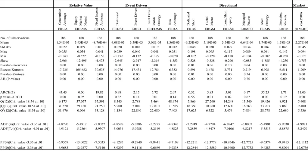
Table 1 contains the descriptive statistics of net-of-fee monthly excess returns (in excess of six month LIBOR rate) of the CSFB/Tremont indices.7 According to the figures in Table 1, the best performing HF style in terms of returns is Global Macro with 0.519 percent average monthly excess return (6.228 percent annualized) for the sample period (1994-2009), while the poorest performing style is Dedicated Short with –0.6237 percent monthly return (-7.476 percent annualized). A comparison of the HF returns with the S&P500 index reveals that only five HF
7 In the literature, various risk-free rates are used to define excess returns. These include LIBOR (Billio et al. 2006),
styles namely, Event Driven, Event Driven Multi-Strategy, Global Macro, and Long-Short Equity, outperformed the broader market index for that time period. The most risky HF style, as measured by standard deviation, is Dedicated Short (SD=0.048), closely followed by Emerging Markets (SD=0.046) while the least risky style is Risk Arbitrage (SD=0.012).8
In all but one instance (Dedicated-Short), the unconditional skewness statistics are negative and with the exception of Managed Futures, the values are all statistically significant. The range of skewness is from 0.528 for Dedicated Short to -12.49 for Equity Market Neutral, demonstrating a wide range of statistical distributions.9 Presence of significant skewness is an indication of asymmetry of the HF return distribution around its mean, contributed to by various option-based investment strategies employed by the HF (Fung and Hsieh 1997). The negative sign of skewness is an indication that the corresponding HF bears significant tail risk and serves as a potential source of contribution to systemic risk. Returns on these HFs may be positive most of the time until a tail event occurs that forces the HF to make large option payouts (large loss).
The excess kurtosis values for all HFs are positive and statistically significant, with the exception of Managed-Futures, indicating that almost all HF return distributions are leptokurtic, demonstrating long tails and extreme values on both sides of the mean. Almost all HFs have negative excess skewness and positive excess kurtosis. Both are undesirable features which need to be compensated with greater premia. The magnitude of excess kurtosis of the HFs is directly proportionate to that of their skewness (Table 1), namely that risky HFs are risky both in terms of skewness and kurtosis and contribute to systemic risk through both channels. In particular, the
8 The lack of normality in distribution has implications for the way HF risks are evaluated. As stated previously,
Brooks and Kat (2002) have argued that investors may receive a higher mean return and lower volatility in return for more negative skewness and higher kurtosis. As a result, some HFs may exhibit low standard deviations, but this may not necessarily imply that they are less risky.
9 The dramatically high skewness and kurtosis for Equity-Market-Neutral style is caused by its performance since
November 2008. The estimated skewness and excess kurtosis during the period of January 1994September 2008 is -0.069 and 0.7975, respectively, which is similar to those obtained by Billio et al. (2009).
Equity-Market-Neutral style has the highest level of skewness as well as the largest level of excess kurtosis. The range of excess kurtosis for the HFs studied is from 0.21 for Managed-Futures to 165.68 for Equity-Market-Neutral and is time dependent10,indicating that these HFs have a more peaked (leptokurtic) distribution than normal and exhibit more extreme values. Using the CSFB/Tremont HF excess return data, as is used in this study, Chan et al. (2005), Billio et al. (2006) and Billio et al. (2009) also find the magnitude of skewness and excess kurtosis to be period-dependent. With the exception of Equity-Market-Neutral, our results are similar to those obtained by Billio et al. (2009). The high excess kurtosis values are consistent with considerable contributions from these HFs to extreme events and, hence, systemic risk.
The ARCH (1) test results reveal the presence of first order ARCH effects in the return series of Convertible Arbitrage, Fixed-Income-Arbitrage, Event Driven Multi Strategy, Global- Macro, and Multi Strategy. However, no evidence of higher order ARCH effects, represented by Q2 (n), is found to be present (Table 1). This means that shocks to HF returns do carry over to the next month but die down at that point. The evidence of limited ARCH effects in monthly data series, supported by Li and Kazemi (2007), does not preclude the presence of long-term persistence as captured by a GARCH process.11
3.2 The Model
3.2.1 Specification of the Model and the Risk Factors
10 The dramatically high kurtosis for Equity-Market-Neutral (165.68) reduces to 0.34 and 0.51, respectively, if the
time period ends in March 2005 and December 2007. The extreme peakedness is caused by the fall in Equity Market Neutral returns by 51.8% in November 2008. Although not as dramatic for other styles, the magnitudes of skewness and kurtosis do vary with the length of the holding period for all HFs.
11 The Jarque-Bera (1981) test for joint normal skewness/kurtosis (zero skewness, zero-excess kurtosis) rejects
normality for all return series, with the exception of Managed Futures. The Ljung-Box (1978) test statistics of 12 lags reveal that the null of zero autocorrelation can be rejected for the return series of Global Macro, Multi Strategy and Risk Arbitrage. To avoid model misspecification problems, the Augmented Dickey-Fuller (ADF) test (Dickey and Fuller, 1979, 1981), and the Phillips-Perron test (Perron, 1988; Phillips and Perron, 1988) are performed to check the stationarity of the HF excess returns series. The findings indicate that all return series are stationary.
It is widely accepted that, to capture the differences in HF management styles, style-specific performance measurement models have to be used (Agarwal and Naik, 2004). Several existing studies have employed the stepwise regression procedure to identify the appropriate factors for each style (e.g., Chan et al., 2005; and Billio et al., 2006). We adopt the factors (Fm,t) so selected by these authors along with co-skewness and co-kurtosis to investigate of HF returns within a four-moment factor-EGARCH (1,1) model described by the system of equations (1) – (4) below:
3 1 2 3 1 1 , 98 07 08 0 , n j m j Rk t b b RMj t f Fm m t d D d D d D t (1) 1 ; ~ (0, , ), ~ (0,1) ( t ) z h t h z iid t t t t t t I , E( ) 0 and (t E t s) 0, t s (2) 1 2 3 log( )ht g z( t1)log(ht-1) D98 _ 07 D07 _ 08 D08 _ 09 (3) ( ) [ - ( )] g zt zt E zt zt (4)
In this model, Rk t, is the excess return on HF style k (k = 1, 2, .,13) at time t. j t
RM (j=1,2,3) are the market premium and its squared and cubed values. The coefficients of the latter two variables represent co-skewness and co-kurtosis, respectively. The risk factors (Fm t, ) for each style are described in appendix1. The financial crises dummy variables, D98, D07, D08, are detailed in the next section.12 All returns are defined in excess of six month LIBOR. Equation (2) describes the error term,t, and its standardized value ztt ht . Equation (3) describes the conditional variance of the error tem (t), namely ht, as an exponential function of g zt( 1)and past
conditional variances (ht-1), where ht is assumed to be time-varying, positive and a measurable function of the information set (t-1) and g zt( 1) is an asymmetric function of zt (equation 4). As Nelson (1991) points out, in order to accommodate the asymmetric relation between return
shocks and volatility changes, the conditional volatility must be a function of both the size and the sign of the standardized residual (zt). In equations (3-4) αzt1E zt1is considered the “size”, the “magnitude”, or the “cluster” effect, whilezt1is the “sign” effect, for the shock zt.
Coefficient , pertaining to the size effect, is expected to be positive indicating that larger shocks to returns will have greater impacts on HF volatility, than smaller shocks, regardless of whether they are positive or negative. If coefficient, pertaining to the “sign effect’ is non-zero (
0
) and statistically significant, the shock impact will be asymmetric because in this case negative and positive values of zt increase the volatility differentially. In particular, when ( 0)
, negative shocks (zt < 0) increase volatility more than positive shocks of equal magnitude.13 The strength of the asymmetry can be measured by the relative contributions of the negative and positive shocks to volatility, or the relative sensitivity of g(z) to shocks when shocks are, respectively, negative and positive. This measure can be calculated as the ratio of the derivatives of g (z) with respect to z under negative and positive shocks, which is derived as: (|-1+γ|)/(1+ γ).14 The asymmetry effect is referred to as the “leverage effect”in the equity literature because it entails that negative innovations reduce the value of equity, thereby, increasing financial leverage and making the equity riskier (increase its volatility). The lagged volatility term log (ht-1) is the GARCH effect. The GARCH coefficient determines the influence of past conditional volatilities on the current conditional volatility, or the persistence effect.
3.2.2 HFs and Financial Crises
13
Nelson (1991) explains the size effect in the following manner. To see that the first component of g(zt) represents a size effect, suppose α > 0 and γ = 0. Then the innovation in log (ht+1) will be positive (negative) when
the magnitude of |zt | is greater (smaller) than its expected value. For the sign effect, suppose α = 0 and γ < 0, then innovation in log (ht+1) is sign-sensitive; it is positive when zt is negative and vice versa. In some cases the overall
change in volatility is indeterminate, e.g., when α > 0 and γ < 0. See Koutmos and Booth (1995) and Nelson (1991). 14See Koutmos and Booth (1995), əg(z)/əz is (1+ γ) for z >0 and (|-1+ γ|) for z <0.
The role of HFs in financial crises has been extensively analyzed (Adams et al., 1998, Eichengreen et al., 1998, Jorion, 2000, Brown, Goetzman and Park, 2000, Fung et al. 2000, and Brown et al., 2009). Although HFs tend to play a considerable role in financial crises, they have been found not to cause them, except, perhaps, the crisis following the Long-Term Capital Management (LTCM).15 To capture the effects of financial crises on HF returns distributions, several crisis event dummies, and three non-overlapping pre-and post event period dummies are used. The event dummy variables are defined as follows:
Financial Crisis of 1998: (D98) =1 for the months of August and September 1998, zero
otherwise. Two major events; the default of Russian government debt in August 1998 and the events surrounding the Long-Term Capital management (LTCM) in September 1998, contributed to an increase in “systemic risk” of HFs (Chan et al., 2005).
ortgage Crisis of 2007: (D07) =1 for October 2007, zero otherwise. Although it is difficult to perfectly ascertain the start of the subprime mortgage crisis, the signs for a major crisis were visible in October 2007. According to Mortgage Bankers Association, in the third quarter of 2007, the sub-prime Adjustable Rate Mortgage (ARM) outstanding, stood only at 6.8%, but represented 43% of the foreclosures. Additionally, in this period the seriously delinquent rate for subprime loans was 460 basis points higher compared to the third quarter 2006 (http://www.mbaa.org/NewsandMedia/ PressCenter/ 58758.htm).
Credit Crisis of 2008: (D08) =1 for September and October 2008, zero otherwise. It is
difficult to perfectly pinpoint the start of the credit crisis in 2008. However, the government takeover of Fannie Mae and Freddie Mac, the merger of Merrill Lynch with Bank of America, the collapse of Lehman Brothers and the bail out of AIG in September and the consequent uncertainty in October are characterized as the credit crisis event.16 Three non-overlapping pre- and post-event dummy variables are included in the volatility model to demarcate the shifts in volatility after each crisis event. They are defined as:
D98_07 = 1 during the period of August 1998 to September 2007, zero otherwise;
D07_08 = 1during the period of October 2007 to August 2008, zero otherwise;
D08_09 = 1 during the period of September 2008 to August 2009, zero otherwise.
15 At the height of Asian financial crisis in 1997, some Asian governments accused HFs of driving down the value
of their currencies (see, Brown et al., 2000). However, studies by Adams et al. (1998), Eichengreen et al. (1998), Brown et al., (2000), and Fung et al., (2000) conclude that the dynamics of HF activities provides little evidence that HFs caused the crisis. Similarly, although the failure of Bear-Sterns HFs did set off the collapse of sub-prime CDOs in 2007, Brown et al. (2009) maintain that HFs did not cause the growth of these CDOs. As such, there is little evidence that HFs caused the 2008 financial crisis.
16 In the extant literature, different lengths of event windows have been used for the LTCM crisis of 1998 (Rigobon,
2003), mortgage crisis of 2007 and credit crisis of 2008 (Billio et al. 2009). We also used shorter/longer windows and non-overlapping dummies for the event. Results, available on request, are identical to those reported in Table 2.
A positive (negative) crisis dummy coefficient i is associated with increased (decreased) level of volatility during the post event period. The parameter vector [ , , , , , , , , ]b b f d0 j m i i is estimated simultaneously by using the maximum likelihood estimation technique.
4. EMPIRICAL RESULTS
4.1 Excess Return, Market, Co-Skewness and Co-kurtosis
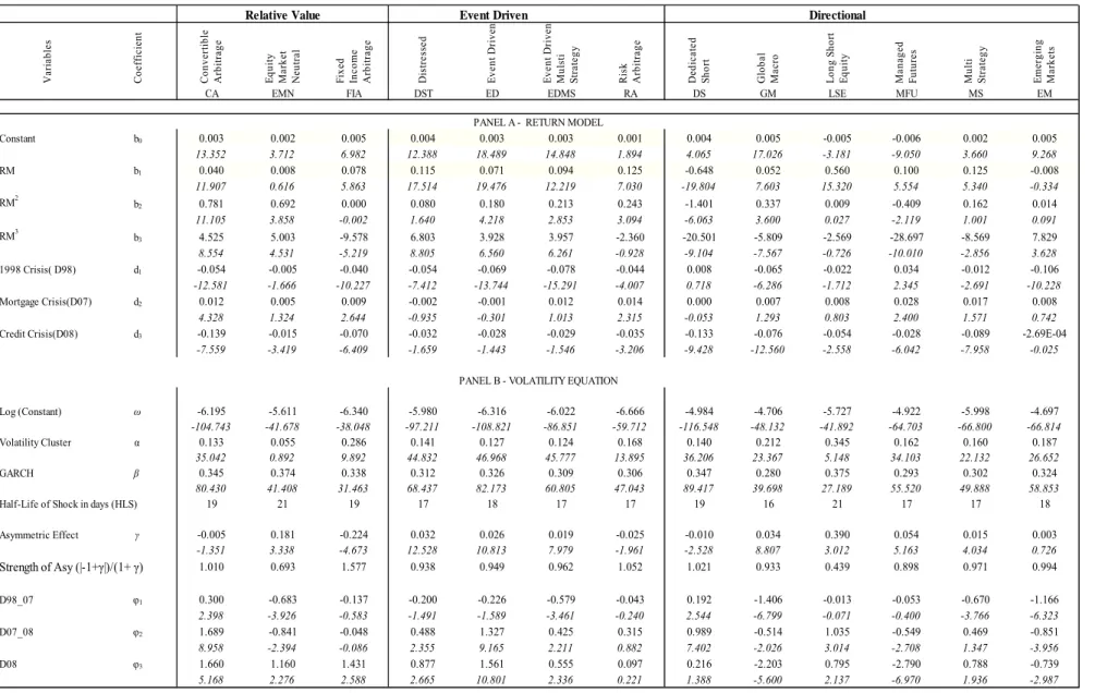
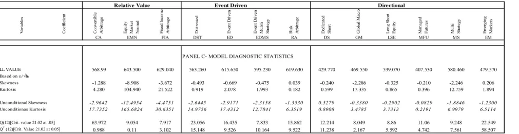
Table 2 presents the higher-moment factor-EGARCH (1,1) results. The intercept represents performance for zero values of co-skewness, co-kurtosis, and risk-factors during the non-crisis period. For each style, the intercept (b0) is highly significant and, with the exception of Long-Short Equity and Managed-Futures, positive, indicating that absent any effects from market, co-skewness, co-kurtosis and risk-factors, HFs did well during the non-crisis period in terms of producing abnormal returns. This indicates market inefficiency and skillfulness of the HF managers. The sensitivity to S&P 500 variable (b1) is statistically significant, suggesting exposure to market and making the title “hedge fund” a misnomer, except for Neutral and Emerging Markets funds. The neutrality to market factor of the Equity-Market-Neutral style is consistent with expectations. However, the Emerging- Markets style that involves investing in both stock and fixed income securities around the world appears to have properly hedged its exposure to the U.S. market as its beta is insignificant as well. Alternatively, it is possible that S&P 500 is not a suitable market factor for the emerging market assets. All market beta coefficients, with the exception of Dedicated-Short, are positive. The negative market exposure of this latter style is because it maintains a net short position, mostly in equities and derivatives, at all times. In terms of the magnitude of the market exposure, the Long-Short Equity, a member of Directional Strategy, has the highest exposure (0.56), due to the speculative nature of its strategy. Convertible- Arbitrage, a part of relative value (or non-directional) strategy
has the lowest exposure (0.04) because this strategy takes advantage of temporary mispricing between different financial instruments and maintains a very low exposure to the market.
The skewness of the market (-0.75) and all HF returns, reported in Table 1, are negative, except for Dedicated-Short, which is positive, and Managed-Futures, which is insignificant. The negative skewness figures indicate that the market and the corresponding HFs were left-skewed and experienced more negative than positive extreme (tail) values over the sample period (which includes the crises periods). The coefficient of co-skewness (b2) is significant for nine out of the thirteen styles studied, with Dedicated-Short and Managed-Futures, part of directional strategy, exhibiting negative co-skewness, and the remaining seven styles showing positive co-skewness. A positive (negative) co-skewness coefficient (b2) indicates that adding the HF to the market portfolio by an investor would produce a portfolio with a less (more) negative skewness, making it more (less) desirable to the investor. Of the seven styles that show positive co-skewness, the co-skewness coefficient is largest for Convertible-Arbitrage (b2=0.781) followed by Equity-Market-Neutral (b2=0.692), both a part of relative value strategy. These HFs enhance the market risk to the largest extent as they reduce the chances of extreme negative returns the most.
HFs with negative co-skewness, namely Dedicated-Short and Managed-Futures, are less desirable because they shift the return distribution to the left and are more likely to make a contribution to financial crisis. The negative co-skewness of Dedicated-Short and Managed-Futures may be, at least partially, due to nature of their assets and the trading strategies they utilize. Dedicated-Short HFs tend to maintain net short position and to hold put options. Managed-Futures HFs also long put options. Trading strategies such as longing put options permit occurrence of small losses on an ongoing basis with infrequent large profits. Anson and Ho (2004) show that Managed-Futures’ commodity trading advisors (CTAs) provide an
exposure whose payoff is similar to a long put option (see Gregoriou et al, 2005, p. 269 for a discussion of option based strategies). These HFs contribute to financial crisis through the skewness channel as they allow for more negative extreme values.
The co-kurtosis coefficient (b3) is significant for eleven out of the thirteen styles, of which five are negative and six are positive. Positive (negative) co-kurtosis of a HF indicates that the HF and market returns tend to share more (fewer) extreme events, heightening (moderating) the risk and contributing more (less) to crises. With the exception of the Emerging-Market style, all significant co-kurtosis coefficients under directional strategy are negative along with the coefficient pertaining to Fixed-Income-Arbitrage under the relative value strategy. In terms of magnitude, the co-kurtosis coefficients of Managed-Futures (b3 = -28.69) and Dedicated-Short (b3 = -20.50) are considerably greater (in absolute term) than other HFs indicating greater impact on the market portfolio. The negative co-kurtosis of these HFs is an indication that they share few extreme events with the market at large, and they make its distribution less peaked. Since this is a desirable property, these HFs have a lower expected returns, though their actual returns are unpredictable. Contrary to this, for HF styles Convertible-Arbitrage, Equity-Market-Neutral, Distressed, Event-Driven, Event-Driven-Multi-Strategy, and Emerging-Markets, the co-kurtosis coefficient (b3) is positive. These HFs tend to share more extreme events with the market, curtailing the diversification benefits and boosting the overall portfolio risk as a result. These HFs are less desirable to risk-averse investors and are, therefore, expected to command higher returns (see, Guidolin and Timmermann (2008) for a discussion). These HFs must be watched more carefully by the regulators because they have the potential to contribute to systemic crisis.
Overall, our results show that skewness and kurtosis are significant factors in describing HF returns behavior, when market is already accounted for, and should be included in returns
modeling. In other words, the market risk measure used in typical asset pricing models is not an exhaustive measure of risk. Inclusion of these higher moments in the model improves the accuracy of return and risk assessment of the HFs and delineation of their contribution to systemic risk. The inclusion of these moments also allows us to better pinpoint the type of risk inherent in the fund. For example, the negative co-skewess and positive co-kurtosis of the Managed-Futures style, found within our extended model is an indication that the risk reduction property of this HF found in the literature within a two-moment framework (Abrams et al., 2009, Schneeweis, 2001), is a combination of variance, co-kewness and co-kurtosis risk categories. Hence, if these higher moments of the return distribution are excluded, pricing, risk measurement, cost of debt and the hedging strategies relevant to these HFs are likely to be distorted. Huber and Ronchetti (2009) have shown that when fat tail error distributions (skewness, kurtosis) are present, OLS estimates will be inefficient. This renders the results in the existing literature based on this technique suspect.17
4.2. Results on HF Volatility Model: Clusters, Asymmetry and Shock Persistence
An advantage of estimating HF volatility within the framework of an EGARCH model is the ability to disaggregate the changes in volatility into cluster effect (size effect), asymmetry (sign or leverage effect) and persistence effects (GARCH). The coefficients ,γ, and β in equations 3-4, describing the conditional volatility process, represent these effects, respectively. 4.2.1. Cluster Patterns
Volatility clustering is said to exist when high (low) HF volatility in a given period is followed by high (low) volatility in subsequent periods. It is important for regulators, investors and corporate managers alike to understand the volatility clustering patterns of HFs because
17 The magnitudes and the directions of the coefficients pertaining to macroeconomic factors that we obtain are
these patterns contribute to the overall pattern of volatility, and, hence, impact asset pricing and hedging strategies.18 Specifically, since the timing and duration of volatility clusters can significantly alter the value of hedging instruments and, consequently, affect the HF’s ability to manage the shifts in volatility, knowledge of clusters is crucial for risk management. We investigate the effects of clustering on HF volatility within our adopted generalized framework.
We find that all HF styles, with the exception of Equity-Market-Neutral, demonstrate positive and significant values of the clustering parameter (α). This indicates that for all HF styles, except one, larger surprises in returns, regardless of their signs, will increase the HF return volatility to a greater extent, than smaller shocks, and high (low) volatility in a given period will be followed by high (low) volatility in subsequent periods (Table 2, panel B). The magnitude of the effect is measured by the term [zt - (E zt)], called the size effect, as it shows the size of the surprise. The highest and lowest significant (α) values pertain to Long-Short Equity (0.345), and Event-Driven-Multi-Strategy (0.124), respectively. The higher (α) value for the Long-Short HF denotes that this HF style is subject to stronger clustering tendencies. Consequently, shocks to this style will heighten its volatility to a larger extent and if its volatility spills over to other styles, the HF industry and the financial system as a whole will be more heavily affected. The speculative nature of the Long-Short Equity strategies; longing in rising markets and shorting in falling markets, is a driving force behind its strong cluster pattern. The significance of cluster patterns for all HFs, except one, is an indication that shocks to HFs do
18 In the aftermath of LTCM crisis, there has been a growing demand on the part of the HF managers for instruments
such as variance swap in order to hedge movements in volatility and to advance revenues. A variance swap used in trading variance risk is a product that allows the buyer to hedge the risk of volatility of an underlying security or index by paying a premium to be able to receive the large positive payoff of a variance swap in times of market turmoil. The seller benefits from the revenues generated through the contract. The largest sellers of the variance risk are Distressed Securities, Emerging Markets, Equity Non-Hedge (not studied here), Event-Driven, and Fixed Income HFs. Bondarenko (2006) finds that on average, the HF industry earns about 6.5% of its total assets annually by short-selling the variance risk ($32.4 billion in 2000).
accelerate in subsequent periods and if there is a common shock to all HFs, the magnitude of the effect on the system will be substantial. This calls for regulators’ close watch of the HF industry. 4.2.2. Asymmetry
As discussed in section 2.2, a main contribution of this study is to identify whether the HF volatility reactions to positive and negative return shocks are asymmetric, i.e., whether the HF volatility is affected differentially by positive and negative shocks to its returns. As detailed earlier (section 3.2.1), given the positive sign of (α) in the function g z( )t [zt - (E zt)]zt
(equation 4), a negative shock (z) will increase volatility to a greater extent when < 0 than when > 0. The relative magnitude of a negative and a positive shock effect on volatility is measured by the ratio 1 / (1). The results, presented in Table 2, panel B, suggest that for two out of the thirteen HF styles studied, Emerging Markets and Convertible Arbitrage, the sign effect coefficient ( ) is insignificant ( = 0) denoting symmetry namely that negative and positive shocks increase volatility to the same extent. For the other eleven styles is highly significant indicating the prevalence of asymmetry. One plausible explanation for finding of symmetry for the Emerging-Market style is that the volatility of emerging equity markets is primarily driven by local factors and these factors may demonstrate symmetric effects because they are less integrated with world markets, have access to fewer types of instruments and are slow to adjust.
The values for the intensity of asymmetry, 1 / (1), are reported in table 2 below values. This ratio shows the extent to which a negative innovation will differentially impact volatility, compared to a positive innovation. For example, using = -0.224 for Fixed-Income Arbitrage, we obtain a ratio of 1.56, indicating that a negative innovation in this HF style will
increase volatility more than a positive innovation by a factor of 1.56 (or 56% greater). In terms of the magnitude of asymmetry (in absolute term), for cases that negative shocks have larger effects, the Fixed-Income Arbitrage exhibits the most asymmetry ( = -0.224, the intensity ratio
= 1.56) while Convertible Arbitrage style exhibits the least asymmetry ( = -.005, the intensity
ratio = 1.01). The implication is that the former is of more concern to the investors and regulators during the market downturns because its decline will be sharper and will impact the system more strongly downward. The Long-Short Equity style exhibits the most asymmetry in the reverse direction, in the sense that negative shocks increase volatility to a much lesser degree (43%), compared to the positive shocks ( = .039, the intensity ratio = .439).
The asymmetry (leverage) effect is prevalent in the equity return literature (Engle and Ng, 1993). However, Braun et al. (1995) report that this effect occurs mainly at the market level while it is limited for industry portfolios. Our findings show that asymmetry is considerable even at the HF portfolio level, at least for some HF styles, and that negative shocks could lead to greater or lesser volatility than positive shocks. Consistent with the equity return literature, we find the asymmetry coefficient to be negative ( 0) for the Fixed-Income-Arbitrage, Risk-Arbitrage and Dedicated-Short HF styles, namely that for these styles, negative shocks (bad news) increase their volatility more so than positive shocks (good news). The implication is that during the downturns these HFs need to be watched more carefully or they should be hedged prior to the downturns to avoid their heavier impact on the industry and the financial system.
There are several possible explanations for a negative relationship between return shocks and return volatility to hold. First, in line with the leverage effect, when the values of these HFs drop due to poor performance, their equity becomes more leveraged, causing the volatility of returns to increase in magnitude. Second, in line with the time-varying risk premium hypothesis
discussed by French et al. (1987), if volatility is priced, an anticipated increase in HF volatility will raise its required rate of return which will lead to an immediate decline in the value of HF assets. A similar explanation is proposed by Bekaert and Wu (2000) within the framework of volatility feedback effect suggesting that if volatility is priced, an anticipated increase in volatility raises the required return on assets, leading to an immediate decline in the asset price. Contrary to the leverage effect, the underlying causality in the time-varying risk premium and volatility feedback approaches run from volatility to price (Bollerslev et al., 2006). Third, if more assets flow into the fund due to better than anticipated performance, HF managers may selectively invest in securities that are safer, or not priced on a daily basis, and, therefore, lower the volatility of the fund. 19
The fining of ( > 0) for the remaining HF styles is similar to that obtained by Braun et al. (1995) at the portfolio level. For these HF styles, positive innovations in returns produce a positive sign effect and they may increase conditional volatility in the next period, to a greater extent than negative shocks. This delineates a tradeoff between return and volatility in the sense that these two variables move in the same directions, as do risk and return.
The co-movement of returns and volatility may occur e.g., if HFs are holding options and as markets rise, the chances of exercising the option increase, leading to greater volatility as well as greater return. In general, HFs utilize various strategies including lock-ups, side pockets, spinouts, various gate provisions, redemptions-in-kind, suspension of redemption, and innovations, to control liquidity (cash outflow) and down-side risk. If HFs receive additional cash inflows, in response to good performance, and these cash flows are blocked from flowing out by the above mechanisms, HFs may become confident in investing in risky assets with higher
returns and higher volatilities, increasing the overall volatility as a result. Moreover, it is well-established in the literature that performance persistence of HFs is short-lived, typically from one quarter up to one year (Agarwal and Naik 2000), suggesting that the assets purchased by the new cash inflows may lead to a decline in performance because assets with the previously prevailing risk-return trade-offs are difficult to attain (Ding et al., 2007). Thus, in an effort to maintain higher returns, the HF manager may seek out assets with greater risk. Conversely, when HFs are faced with negative shocks, they will not be harmed by cash outflows and they may, in addition, become more risk averse, making safer investments and lowering volatility.
4.2.3. Shock Persistence
Panel B of Table 2 presents the parameters of the conditional volatility model (equation 3). The GARCH coefficient,, determines the influence of the past conditional volatilities on the current conditional variance, or how strongly volatility shocks persist from one period to the next. Results presented in Table 2 show that the necessary stationary condition 1is met for all HF styles. The strength of the volatility persistence () stands at approximately 0.3 for all HF styles, indicating that 30% of the volatility shock sustains itself from one period to the next and 2.7% (.33) of the shock is sustained after 3 months.
An alternative measure of volatility persistence is the half-life of a volatility shock (HLS), which is the time it takes for the volatility to move halfway back towards its unconditional variance after it receives a shock (Engle and Bollerslev, 1986). HLS can be measured as: HLS Ln 0.5 /Ln β .20 The EGARCH volatility process employed here is considered to be “mean reverting” to its long-run level with the magnitude of controlling the speed of the mean reversion. The HLS values for the HFs considered are produced in Table 2
below the GARCH parameter (). As an example, for Convertible-Arbitrage (=0.345), the HLS is Ln(0.5) Ln(0.345) = 0.65 of a month, or approximately 19 days. This indicates that once a shock is introduced to this HF, it will take 19 days for the volatility to move halfway back towards its unconditional variance. Utilizing the same approach, the HLS for each strategy is found to be between 16 days for Global-Macro (as the fastest reversion case) and 21 days (for Equity-Market-Neutral and Long-Short Equity as the slowest cases). The fitted EGARCH models strongly suggest that the shocks to HF returns are relatively short-lived, compared to their equity counterparts which show persistence of six to twelve months according to Bollerslev et al., (1992).21 It is notable, however, that the sample period of the latter study occurred earlier in time, when markets were slower to adjust.22
4.2.4. Similarity in Volatility Patterns across HFs
An interesting issue is the degree of similarity of the changes in volatility patterns across HFs, including clusters, asymmetry and shock persistence, because these similarities can accentuate the effect of shocks and lead to crisis. These effects are of concern to investors, especially institutional investors such as banks, pension funds, mutual funds, insurance companies, HF managers and regulators in choosing the
portfolio mix, hedging decisions and the design of the regulatory structure. Similarity in
cluster patterns can be examined by comparing the cluster parameter (α) across HFs. If cluster patterns are similar across HFs, the effects of shocks on different HFs will follow parallel patterns, rather than being staggered or counterbalancing. These effects will ebb and spike
21 A wide variety of equity indices are studied. For example, Nelson (1991) used CRSP Value-Weighted Market
Index while Engle and NG (1993) used the Japanese TOPIX index.
22 To investigate whether shock half lives (HLS) shortened or lengthened during the recent crisis, we also run
identical models with data set ending in 2005. The magnitudes of all HF betas are approximately 0.3, and, hence, HLS values, remain around 17 days.
simultaneously, producing sharper bumps and valleys in the aggregate and in systemic risk measures. Cluster patterns examined here show a moderate degree of similarity as for ten, out of the thirteen, HFs parameter (α) takes a value between zero and .2 with even the three exception cases being close to this range (Global Macro .21, Fixed-Income Arbitrage .28, Long-Short Equity .35). The rather low value of (α) indicates a mild tendency to cluster.
Asymmetry also demonstrates similarity across HFs as for ten out of the thirteen HFs considered the asymmetry parameter (γ) varies over a narrow range (0.0-.05), despite the idiosyncratic volatility characteristics that are inherent in each HF style. The three exception cases are Equity-Market-Neutral (γ = .18), Fixed-Income-Arbitrage (γ = -.22) and Long-Short Equity (γ = .39). The relative strength of asymmetry ( 1 / (1)) shows a greater range of variation, however. HFs show a greater degree of similarity in terms of shock persistence as (β) parameters are similar in magnitude and the HLS for all HF styles is limited between 16-19 days. In terms of implications for the systemic risk, the finding of similarity in volatility patterns and persistence of shocks across HFs indicates that the effect of a general shock to all HFs would continue over the same length of time, namely that parallel effects on different HFs would make the cumulative impact on the industry and the financial system large, and then, at a certain point in time, the effects would disappear within a few days across all HFs, creating a sharp movement in the opposite direction. This pattern is likely to cause high volatility and strengthen systemic risk.
We also investigate the co-dependence of HF return volatilities employing a variance decomposition framework (VDC). HF return volatilities may be driven fully by their own internal dynamics (segregation hypothesis) or, at least partially, by outside factors such as spillovers of shocks from other HFs, in particular, HFs within the same strategy
(interdependence hypothesis). Hence, we conduct the VDC within each of the HF strategies (Relative Value, Event Driven, and Directional). According to the results (not reported), different HFs are differentially susceptible to volatility changes in other HFs within their own strategy. For example, within the first three months after a shock is introduced, internal dynamics determine around 80%-90% of the volatility variation in eight of the thirteen HFs, an indication that internal forces are the dominant drivers of volatility variation. This figure is between 65%-80% for another two funds and 45%-63% for the remainder three funds. Outside forces, namely spillovers from other HFs from the same strategy, constitute the remaining share of the volatility changes. The greater degree of interdependence in volatilities (lowest share contributed by internal dynamics) in the latter three cases tends to amplify the effect of shocks on the overall market and lead to a greater systemic risk. These three funds, all from the Event Driven strategy, are clearly more exposed to external shocks. Overall, the degree of interdependence across HFs, as revealed by the VDC, is also moderate in nature and should not be considered alarming in terms of contribution to systemic risk.
4.3. Performance and Risk under Crisis Conditions 4.3.1. Effect of Crisis on HF Returns
The return model (equation 1) includes three event dummy variables for the three crises which occurred during the sample period; the Russian debt crisis of 1998 which coincided with the collapse of LTCM, the mortgage crisis of 2007 and the credit crisis of 2008. Our results, displayed in Table 2, panel A, show that the Russian and LTCM debacles did materially affect HF returns. The coefficients pertaining to this crisis (D98) in the mean equation of all HFs, with the exception of Dedicated-Short, are highly significant. The direction of the effect is negative in all cases, except Managed-Futures, indicating that all HF styles, except one, were unprepared for the Russian and the LTCM crises and sustained losses as a result. These effects may be of a pure
contagion type, based on fear, or an information-based effect due to common positions taken by the HFs in the sample at the time of the crisis. The exceptions, namely Managed-Futures and Dedicated-Short, are likely to have had enough short positions to counterbalance the losses and they also tend to display low or even negative correlation with equity returns. The Emerging Markets style sustained the greatest loss during this crisis, as measured by the coefficient (d1) of
-0.106, perhaps because of difficulties in hedging such positions, while Equity-Market-Neutral style sustained the lowest loss with a coefficient of -0.005, as it should be expected. Managed-Futures HF, which has historically exhibited low or even negative correlation with traditional investments and generated strong absolute returns across market cycles, enjoyed a gain, as shown by a coefficient value of 0.034.23
The nature of the trading strategies utilized by the managers often creates additional diversification benefits. Most Managed-Futures programs use disciplined, trend-following trading strategies which are designed to capture a majority of the price movements in long and intermediate-term trends while systematically using stop-loss orders to try to exit bad trades before the losses pile up (turtletrader.com/pdfs/managed_futures.pdf). It appears that at times of market distress, Managed-Futures HFs provided a valuable channel of diversification for investors because of their investments in a wide range of markets/instruments and their managers’ skills.24
According to the results shown in Table 2, ten of the thirteen HF styles were significantly affected by the credit crisis of 2008, accounted for by the dummy variable D08, and the effects were all negative. It seems that the HFs in none of these ten styles were ready to confront the crisis as they had not expected it, nor taken steps to cover themselves against this type of shock.
23 See Lintner (1983) for a discussion of portfolio diversification using Managed-Futures investments.
24 A number of HF styles rebounded by June 1999. The styles such as Equity-Market-Neutral, Long-Short Equity
and Managed-Futures posted returns greater than 15% while Event-Driven and Multi-Strategy HFs showed smaller though positive returns. However, Dedicated-Short, Emerging-Markets and Global-Macro styles remained in the negative territory. (http://www.hedgeindex.com/hedgeindex/documents/Analyzing_Turmoil_ Outcome.pdf).
This finding is supported by Billio et al. (2009) who identified the presence of a common idiosyncratic risk factor for the whole HF industry and found that a latent factor exposure was present during the 1998 and 2008 crises, though not for the 2007 crisis. Billio et al. (2009) conclude that the common latent risk factor and changes in HF risk exposures during this crisis must be included in modeling HF risk. Otherwise, the effect of this crisis on HF risk will be underestimated and the diversification benefits will be exaggerated. Similar to our finding, they conclude that the subprime mortgage crisis affected only a select number of HF styles.
In terms of magnitude, the effect of credit crisis of 2008 (D08) on the HF industry was much more substantive than that of the 2007 mortgage crisis (D07) in all HF styles considered, with the exception of the Emerging-Market. This is reasonable given that HFs were not as highly involved in real estate or mortgages as in stocks, fixed-income instruments and derivatives, and that the negative psychology of markets had clearly deepened in this later stage of the crisis. Furthermore, it is interesting to note that the coefficient of the dummy variable (D07) for the mortgage crisis (d2) is positive and significant for four HF styles: Convertible-Arbitrage,
Fixed-Income-Arbitrage, Risk-Arbitrage, and Managed-Futures. These HF styles appear to have recognized the low quality of the U.S. home mortgage loans, bet against them and profited from their decision.25 The other nine HF styles also escaped unscathed and overall no HF style included in the sample seems to have been harmed significantly by the mortgage crisis which preceded the financial market crisis.
Market developments over the two crises proceeded as follows. From the beginning of the subprime crisis in September 2007, banks, securities firms, HFs and other financial
25 There is additional evidence that a number of HFs posted substantial gains by placing bets against subprime
mortgage securities. The California-based Lahde Capital Management LLC’s US Residential Real Estate Hedge V Class A posted a 1000% return in 2007, making it one of the best performing funds of all time. Similarly, the New York based Paulson & Co. managed to double its assets to $24 billion in 2007. Paulson outperformed most peers in 2007 by betting against collateralized debt obligations (hedgefundhub.com/paulson-co-hedge-fund).
institutions started deleveraging their positions by selling assets, including financial instruments and non-core businesses.26 This unwinding of positions resulted in a cascading price decline across all financial markets (Brunnermeier 2009).27 As asset prices fell, the resulting margin calls forced HFs to offload their liquid assets, in turn triggering further selling pressure and further decline in asset values. In this context, the fact that financial leverage can magnify a small profit opportunity into a large one, and a small loss into a colossal one, played a significant role. As the decline in asset prices reduced the value of the collaterals, credit was withdrawn quickly, leading to forced liquidation of large positions over a short period of time, resulting in a widespread financial panic at this later stage of financial crisis. Thus, the coefficients for the dummy variable for the 2008 credit crisis (d3) are uniformly negative, and with the exception of the Event-Driven,
Event-Driven-Multi-Strategy and Emerging-Markets, they are all statistically significant. Two strategies, Convertible-Arbitrage and Dedicated-Short, sustained the largest negative effects (d3
-0.13), as detailed below, while Equity-Market-Neutral suffered the least (d3 = -0.015). Over
81% of Convertible-Arbitrage managers generated positive returns in 2007. However, none could remain in positive territory as they faced the events of September and October 2008 when the crisis had deepened far beyond their expectations.28
The events surrounding nationalization of Fannie Mae and Freddie Mac and the bankruptcy of Lehman Brothers, both during September 2008, and subsequent implementation of short sale ban at the global level soon after, contributed much to the losses sustained by Dedicated-Short and Convertible-Arbitrage styles. Specifically, with government takeover of Fannie Mae and Freddie Mac and the collapse of Lehman Brothers, which were significant
26 See (gao.gov/new.items/d10555t.pdf). The same GAO report finds that in the fourth quarter of 2008,
broker-dealers reduced assets by nearly $785 billion and banks reduced bank credit by nearly $84 billion.
27 See Brunnermeier (2009) for a discussion on how deleveraging by financial institutions by selling financial assets
and restricting new lending may have contributed to the financial crisis.