Turing Incomputable Computation

(1)

Turing Incomputable Computation

Michael Stephen Fiske

Aemea Institute, San Francisco, California, U.S.A. [email protected]

Abstract

A new computing model, called the active element machine (AEM), is presented that demonstrates Turing incomputable computation using quantum random input. The AEM deterministically executes a universal Turing machine (UTM) programηwith random ac-tive element firing patterns. These firing patterns are Turing incomputable when the AEM executes a UTM having an unbounded number of computable steps. For an unbounded number of computable steps, if zero information is revealed to an adversary about the AEM’s representation of the UTM’s state and tape and the quantum random bits that help determineη’s computation and zero information is revealed about the dynamic con-nections between the active elements, then there does not exist a “reverse engineer” Turing machine that can map the random firing patterns back to the sequence of UTM instruc-tions. This casts a new light on Turing’s notion of acomputational procedure. In practical terms, these methods present an opportunity to build a new class of computing machines where the program’s computational steps are hidden. This non-Turing computing behavior may be useful in cybersecurity and in other areas such as machine learning where multiple, dynamic interpretations of firing patterns may be applicable.

1 Introduction

Recent cyberattacks have demonstrated that current approaches to the malware problem (e.g., detection) are inadequate. This is not surprising as malware detection is Turing undecidable [6]. Further, some recent malware implementations use NP problems to encrypt and hide the malware [17]. Two goals guide an alternative approach: (a) Program execution should hide computational steps in order to hinder “reverse engineering” efforts by malware hackers; (b) New computational models should be explored that make it more difficult to hijack the purpose of program execution. The methods explained here pertain to (a).

Turing incomputable ([4], [7], [8]) computation is created using quantum random input. A new computing machine, called the active element machine (AEM), is presented that uses quantum randomness ([42], [43]) to deterministically execute a universal Turing machine (UTM)

programη(table 2) with random firing interpretations. The active element machine computing

model was introduced in [18], is summarized in section 2 and is further described in subsection 7.2 of the appendix. Furthermore, the active element firing patterns – computing the execution of the UTM program – are Turing incomputable when the UTM computation is non-halting or when the UTM computation is executed repeatedly on an unbounded number of computable initial configurations that halt.

The incomputability of the firing patterns depends on two quantum randomness axioms. 1. No bias. A single outcomexiof a bit sequence (x1x2. . .) generated by quantum

random-ness is unbiased: P(xi= 1) =P(xi= 0) = 1₂.

2. History has no effect on the next event. Each outcome xi is independent of the history.

No correlation exists between previous or future outcomes. P(xi = 1 | x1 = b1, . . . ,

(2)

Let Ω = {(b1b2. . .) :bi ∈ {0,1}} be the space of infinite sequences of 0’s and 1’s

represent-ing infinite quantum random bit sequences. From these two axioms, in [4] Calude and Szovil conclude that if a quantum system producing the quantum randomness runs under ideal condi-tions to infinity, then the resulting infinite sequence of 0’s and 1’s (i.e., sequence in Ω) is Turing incomputable. In other words, no Turing machine can exactly reproduce this infinite sequence of 0’s and 1’s. In this context, no Turing machine can reproduce an unbounded number of the aforementioned active element firing patterns.

The following definition helps clarify the one-way nature of the random AEM firing patterns.

Definition 1. Turing machine map back. Let g : N → {0,1} and f : N → {0,1, . . . , m}

be functions. A Turing machine maps g back to function f if conditions A andB hold. A)

The initial Turing machine tape hasg(k) stored on tape square k for eachk. B)The Turing machine begins execution at tape square 1 and after a finite number of steps writes f(1) on tape square 1. For eachk, the Turing machine visits tape squarekand after a finite number of steps, it writesf(k) on tape squarek and then moves to tape squarek+ 1.

If zero information is revealed to an adversary about the AEM’s representation of the UTM’s

state and tape and the quantum random bits that help determine η’s computation and zero

information is revealed about the dynamic connections between the active elements, then there does not exist a “reverse engineer” Turing machine that can map the random firing patterns back to the sequence of UTM instructions when the UTM executes an unbounded number of computable steps. Overall, using quantum randomness, a finite active element machine can deterministically execute any Turing machine with active element firing patterns that are Turing incomputable. This casts a new light on the notion of acomputational procedure([5], [45]). In [29], Lewis and Papadimitriou discuss the Church-Turing notion of an algorithm (computational procedure):

The principle that Turing machines are formal versions of algorithms and that no computational procedure will be considered as an algorithm unless it can be presented as a Turing machine is known as Church’s thesis or the Church-Turing Thesis. It is a thesis, not a theorem, because it is not a mathematical result: It simply asserts that a certain informal concept corresponds to a certain mathematical object. It is theoretically possible, however, that Church’s thesis could be overthrown at some future date, if someone were to propose an alternative model of computation that was publicly acceptable as fulfilling the requirement offinite labor at each stepand yet was provably capable of carrying out computations that cannot be carried out by any Turing machine.

The works of [14], [22], [23], [27] and [40] describe methods of hypercomputationthat cur-rently have no physical realization. In [11] Davis provides counterarguments to the physical realizability of hypercomputation. In [10] he calls hypercomputation “a myth” and appears to dismiss random number generators as a means to enhance the computing power of Turing machines.

The computing power of Turing machines provided with a random number generator was studied in the classic paper [12]. It turned out that such machines could compute only functions that are already computable by ordinary Turing machines.

In [12], de Leeuw et al. explain that their results depend on the definitions of the machines chosen and the tasks these machines perform.

The following question will be considered in this paper: Is there anything that can be done by a machine with a random element but not by a deterministic machine?

The question as it stands is, of course, too vague to be amenable to mathematical analysis. In what follows, it must be delimited in two respects. A precise definition of the class of machine to be considered must be given and an equally precise definition must be given of the tasks which they are to perform. It is clear that the nature of our results will depend strongly on these two choices and therefore our answer is not to be interpreted as a complete solution of the originally posed informal question.

(3)

What are relevant differences? In [12], the Turing machine reads a random infinite sequence of 0’s and 1’s off the tape – called a probabilistic machine – but the Turing machine program

does not change as a consequence of this random input. (A definition of Turing machine

programis in section 7.1 of the appendix.) In this paper, during AEM program execution, the

Metacommand changes the AEM architecture (program) based on the quantum random input,

which changes the AEM program’s computing behavior. In particular, at each computational step of the UTM, the random input helps determine the element parameters and connection

parameters of the active elements that collectively computeη; and the Meta command helps

dynamically change these parameters based on the random input.

Another AEM example with random input also illustrates the differences. In [18], section

7 describes a method – using a finite AEM program, a quantum random input and the Meta

command – for recognizing a non-Turing binary language L ⊂ {0,1}∗_{. After the AEM has}

received enough random input, then the AEM can determine whether, for example, if the

string 011001 is in the binary languageLrecognized by the AEM. In other words, the random

input helps determine the binary languageL and theMeta command helps dynamically build

the appropriate AEM that recognizesL.

A physical realization of the methods shown here can be implemented using a quantum random generator device [43] with a USB plug connected to a laptop computer executing a finite active element machine program. It is important to note that this physical realization of incomputable firing patterns is a scientific thesis – not a mathematical proof, as this realization depends on quantum theory.

In a cryptographic system, Claude Shannon [38] defines the notion ofperfect secrecy.

Perfect Secrecy is defined by requiring of a system that after a cryptogram is intercepted by the enemy thea posterioriprobabilities of this cryptogram representing various messages be identically the same as thea prioriprobabilities of the same messages before the interception.

Perfect secrecy here means that zero information is released about the state and the tape

contents of the universal Turing machine, the quantum random bits that help determine howη

is computed and the dynamic connections of the active element machine. Formally, letf1,j f2,j . . . fm,j represent the random firing pattern computingη during thejth computational step

and assume an adversary can only eavesdrop onf1,j f2,j . . . fm,j. Letq denote the current

state of the UTM, ak a UTM alphabet symbol andqk a UTM state. Perfect secrecy means

that probabilitiesP(q=qk | f1,j =b1 . . . fm,j =bm) =P(q=qk) andP(Tk =ak |f1,j =b1

. . . fm,j =bm) =P(Tk =ak) for eachbi∈ {0,1} and eachTk which represents the contents of

thekth tape square.

In [28], Kocher et al. present differential power analysis. Differential power analysis ob-tains information about cryptographic computations executed by register machine hardware, by statistically analyzing the electromagnetic radiation leaked by the hardware during its com-putation. If a quantum active element computing system is built so that its internal components remain close to perfectly secret, then it could be extremely challenging for an adversary to carry out cyberattacks such as differential power analysis.

1.1 Brief Summary of Prior Computing Models

In [45], the Turing Machine is introduced. A brief review is in the appendix. In [44], Sturgis and Shepherdson show the computational equivalence of the register machine. The works [9],

[29], [30], [31], [33] and [41] cover computability theory. Alternative models influenced by

neurophysiology are discussed by McCulloch and Pitts in [32], Rosenblatt in [37], Minsky and Papert in [34], Rall in [35], Hertz et al. in [21] and Hopfield in [24], [26] and [25]. In [20] Halang

(4)

et al. describe some advantages of using time. Important work on quantum computing models is presented in [1], [2], [13], [15], [16], [19], [30], [31] and [39].

2 An Informal Summary of the Active Element Machine

A formal introduction to the active element machine is in section 7.2. An AEM is composed of computational primitives called active elements. There are three kinds of active elements: Input, Computational and Output active elements. Input active elements process information received from the environment or another active element machine. Computational active ele-ments receive pulses from the input active eleele-ments and other computational active eleele-ments and transmit new pulses to computational and output active elements. The output active ele-ments receive pulses from the input and computational active eleele-ments. Every active element is active in the sense that each one can receive and transmit pulses simultaneously.

Each pulse has an amplitude and a width, representing how long the pulse amplitude lasts as input to the active element receiving the pulse. If active elementEi simultaneously receives

pulses with amplitudes summing to a value greater than Ei’s threshold and Ei’s refractory

period has expired, thenEi fires. WhenEi fires, it sends pulses to other active elements. IfEi

fires at timet, a pulse reaches elementEk at time t+τik where τik is the transmission time

from elementEi to Ek.

The AEM programming language has 5 commands and 2 special keywords. (See 7.3.)

Con-sider element command (Element (Time 2) (Name L) (Threshold -3) (Refractory 2) (Last 0)). At

time 2, if active element Ldoes not exist, then it is created. Element Lhas its threshold set to −3, its refractory period set to 2, and its last time fired set to 0. After time 2, element L

exists indefinitely with threshold = −3, refractory = 2 until a new element command whose

name valueLis executed at a later time; in this case, the parameter values specified in the new command are updated.

A connection command sets the pulse parameters between two elements. Consider command (Connection (Time 2) (From C) (To L) (Amp -7) (Width 6) (Delay 3)) . At time 2, the connection from active element Cto active element Lhas its amplitude set to −7, its pulse width set to

6, and transmission time set to 3. AFire command fires an input active element in order to

communicate program input to the AEM.(Fire (Time 3) (Name C)) causes element Cto fire at

timet= 3.

AProgramcommand enables one command to execute multiple commands. The execution of(Q (Args 0 E L)) based on the following program definition

(Program Q (Args t x y)

(Element (Time t) (Name x) (Refractory 7) (Threshold 8) (Last 0)) (Connection (Time t) (From x) (To y) (Amp 5) (Width 3) (Delay 4)) )

creates elementEand a connection fromEtoLat timet= 0.

TheMetacommand(Meta (Name E) (Window 1 5) (C (Args a b)) ) causes commandCto

exe-cute with argumentsaandbeach time that elementEfires during the time window [1,5]. The

keyworddTdenotes an infinitesimal amount of time that helps coordinate almost simultaneous

events. dT>0 anddTis less than every positive rational number. The keywordclockevaluates to an integer, which is the current time of the AEM clock.

(5)

3 AEM Interpretations of Boolean Functions

In this section, the same boolean function is computed by two or more distinct active element firing patterns, which can be executed at two distinct times or by two different circuits in the AEM. The use of level sets helps design distinct AEM firing patterns that can compute the same boolean function. These firing patterns can be generated using quantum randomness.

The following procedure uses a finite active element program and a quantum system to either fire input element I or not fireI at time t =n where n is a natural number {0,1,2,3, . . .}. This random sequence of 0’s and 1’s can be generated by quantum systems discussed in [3], [42] or [43].

Procedure 1. Randomness generates an AEM, representing a real number in[0,1] A random sequence of bits creates active elements named 0,1,2, . . . that store the binary representationb0b1b2. . . of real numberx∈[0,1]. If input elementIfires at time t=n, then

bn = 1; thus, create active element n so that after t = n, element n fires every unit of time

indefinitely. If input elementIdoesn’t fire at timet=n, thenbn = 0 and active elementnis

created so that it never fires. The following programrealexhibits this behavior. (Program real (Args t)

(Connection (Time t) (From I) (To t) (Amp 2) (Width 1) (Delay 1)) (Connection (Time t+1+dT) (From I) (To t) (Amp 0))

(Connection (Time t) (From t) (To t) (Amp 2) (Width 1) (Delay 1)) ) (Element (Time clock) (Name clock) (Threshold 1) (Refractory 1) (Last -1)) (Meta (Name I) (real (Args clock)))

Suppose the sequence of random bits begins with 1, 0, 1,. . .. Thus, input elementI fires at times 0, 2, . . . . At time 0, the following commands are executed.

(Element (Time 0) (Name 0) (Threshold 1) (Refractory 1) (Last -1)) (real (Args 0))

The execution of(real (Args 0)) causes three connection commands to execute.

(Connection (Time 0) (From I) (To 0) (Amp 2) (Width 1) (Delay 1)) (Connection (Time 1+dT) (From I) (To 0) (Amp 0))

(Connection (Time 0) (From 0) (To 0) (Amp 2) (Width 1) (Delay 1))

At time 0, input elementIsends a pulse with amplitude 2 to element0. Thus, element0fires at

time 1. At time1+dT, a moment after time 1, the connection from input elementIto element

0 is removed. At time 0, a connection from element 0 to itself with amplitude 2 is created.

Element0continues to fire indefinitely, indicating that b0= 1.

(Element (Time 1) (Name 1) (Threshold 1) (Refractory 1) (Last -1)) is created at time 1. Since element1has no connections into it and threshold 1, it never fires. Thusb1= 0.

3.1 Active Element Firing Patterns

This subsection explains how a firing pattern can be used to compute a boolean function f : {0,1}2 _{→ {}₀_,₁_}_{. These methods can be extended to} _f _: _{₀_,₁_}n _{→ {}₀_,₁_}_{. In the next}

section, the level set methods described here are combined with procedure 1 so that a quantum random firing pattern computes the boolean functions representing the execution of universal

Turing machine programη.

Active elementsX0, X1, X2 andX3 are designed so that eachXi either fires or doesn’t fire

during windowW= [a, b]. After one of the 16 firing patterns is randomly generated, level sets f−1{0}andf−1{1}are used to computef :{0,1}2_{→ {}₀_,₁_}_{. Element}_P _{represents the output}

off. The goal is forP to fire during windowWif and only ifP receives a unique firing pattern from elementsX0, X1, X2 andX3. This goal motivates the following definition.

(6)

Definition 2. Number of Firings during a Window

Let X denote the set of active elements{X0, X1, . . . , Xn−1}that determine a firing pattern during window of timeW. Then|(Xk,W)|=the number of times that elementXk fired during

W. Thus, define the number of firings during windowW as|(X,W)|=Pn−1

k=0|(Xk,W)|.

Observe that|(X,W)|= 0 for firing pattern 0000 and|(X,W)|= 2 for firing pattern 0101. To isolate a firing pattern so that elementP only fires if this unique firing pattern occurs, set the threshold of elementP = 2|(X,W)| −1. The element command forPis

(Element (Time a-dT) (Name P) (Threshold 2|(X, W)| −1) (Refractory b-a) (Last 2a-b))

Each connection fromXk toP is based on whetherXk is supposed to fire or not fire during

W. IfXk is supposed to fire duringW, the following connection is established.

(Connection (Time a-dT) (From X_k) (To P) (Amp 2) (Width b-a) (Delay 1))

IfXk is not supposed to fire duringW, then the following connection is established.

(Connection (Time a-dT) (From X_k) (To P) (Amp -2) (Width b-a) (Delay 1)) The firing pattern is already known because it is determined based on a random source of bits received by input elements, as explained in procedure 1.

Example 1. Computing ⊕with Firing Pattern0010

Firing pattern0010 computes exclusive-orA⊕B= (A∨B)∧(¬A∨ ¬B).

An AEM program is designed such that A⊕B = 1 if and only if the firing pattern for

X0, X1, X2, X3 is 0010. If A⊕B = 1 then P fires. If A⊕B = 0 then P doesn’t fire.

Choose window W = [2,3]. The following commands connect elements Aand B to elements

X0, X1, X2, X3.

(Connection (Time 0) (From A) (To X_0) (Amp 2) (Width 2) (Delay 2)) (Connection (Time 0) (From B) (To X_0) (Amp 2) (Width 2) (Delay 2)) (Element (Time 0) (Name X_0) (Threshold 3) (Refractory 1) (Last 1))

(Connection (Time 0) (From A) (To X_1) (Amp -2) (Width 2) (Delay 2)) (Connection (Time 0) (From B) (To X_1) (Amp -2) (Width 2) (Delay 2)) (Element (Time 0) (Name X_1) (Threshold -1) (Refractory 1) (Last 1))

There are four cases forA⊕B shown below.

1. 1⊕0. ElementAfires at timet= 0 and elementB doesn’t fire att= 0.

2. 0⊕1. ElementsAdoesn’t fire att= 0 and elementB fires at timet= 0.

3. 1⊕1. ElementAfires at timet= 0 and elementB fires att= 0.

4. 0⊕0. ElementsAandB both don’t fire att= 0.

To isolate firing pattern 0010, set the threshold ofPto 2|(X,W)|−1 = 1. The element command forP is (Element (Time 2-dT) (Name P) (Threshold 1) (Refractory 1) (Last 1)). To makeP fire if

(7)

(Connection (Time 2-dT) (From X_0) (To P) (Amp -2) (Width 1) (Delay 1)) (Connection (Time 2-dT) (From X_1) (To P) (Amp -2) (Width 1) (Delay 1)) (Connection (Time 2-dT) (From X_2) (To P) (Amp 2) (Width 1) (Delay 1)) (Connection (Time 2-dT) (From X_3) (To P) (Amp -2) (Width 1) (Delay 1))

For cases 1 and 2, (1⊕0 and 0⊕1) onlyX2 fires. A moment beforeX2fires att= 2 (i.e., −dT), the amplitude fromX2to P is set to 2. At time t= 2, a pulse with amplitude 2 is sent

from X2 to P, so P fires at time t = 3 since its threshold = 1. In other words, 1⊕0 = 1 or

0⊕1 = 1 has been computed. For case 3, (1⊕1),X0, X2 andX3fire. Thus, two pulses each

with amplitude =−2 are sent fromX0 andX3 to P. And one pulse with amplitude 2 is sent

fromX2 toP. Thus,P doesn’t fire. In other words, 1⊕1 = 0 has been computed. For case 4,

(0⊕0),X1 fires. One pulse with amplitude =−2 is sent toX2. Thus,P doesn’t fire. In other

words, 0⊕0 = 0 has been computed.

As shown in table 1, any of the sixteen boolean functions can be mapped to one of the sixteen firing patterns by an appropriate AEM program using level sets to separate elements of the domain {(0,0),(1,0),(0,1),(1,1)}. Each active element Xk in the firing pattern

sep-arates these members based on the (amplitude from A to Xk, amplitude from B to Xk,

threshold of Xk, element Xk) quadruplet. For example, the quadruplet (0,2,1, X1) separates {(1,1),(0,1)} from {(1,0),(0,0)} with respect to X1. Recall that A = 1 means A fires and

B = 1 means B fires. Then X1 will fire with inputs{(1,1),(0,1)} and X1 will not fire with

inputs{(1,0),(0,0)}. The separation rule is expressed as (0,2,1, X1) ↔ _{{₍₁(1_,,₀₎1),_,(0₍₀,_,1)₀₎}_} The

sep-aration rule (0,−2,−1, X2) ↔ {_{₍₁(1,_,0)₁₎,_,(0₍₀_,,0)₁₎}_} indicates thatX2 has threshold−1 and amplitudes

0 and−2 from Aand B respectively. Further, X2 will fire with inputs{(1,0),(0,0)} and will

not fire with inputs{(1,1),(0,1)}.

Table 1: Functionsfk:{0,1} × {0,1} → {0,1} Boolean Function AEM Separation Rule(s)

f1(A,B) = 1 (0,0,−1, Xk)

↔

{(0,0),(1,0),(0,1),(1,1)} ∅ f2(A,B) = 0 (0,0,1, Xk)

↔

_{(0_,₀₎_,₍₁_,₀₎∅_,₍₀_,₁₎_,₍₁_,_1)} f3(A,B) =A (2,0,1, Xk)

↔

{(1,1),(1,0)} {(0,1),(0,0)} f4(A,B) =B (0,2,1, Xk)

↔

{(1,1),(0,1)} {(1,0),(0,0)} f5(A,B) =¬A (−2,0,−1, Xk)

↔

{(0,1),(0,0)} {(1,1),(1,0)} f6(A,B) =¬B (0,−2,−1, Xk)

↔

{(1,0),(0,0)} {(1,1),(0,1)} f7(A,B) =A∧B (2,2,3, Xk)

↔

{(1,1)} {(1,0),(0,1),(0,0)} f8(A,B) =A∨B (2,2,1, Xk)

↔

{(1,0),(0,1),(1,1)} {(0,0)} f9(A,B) =A→B (−4,2,−3, Xk)

↔

{(0,0),(0,1),(1,1)} {(1,0)} f10(A,B) =A←B (2,−4,−3, Xk)

↔

{(0,0),(1,0),(1,1)} {(0,1)} f11(A,B) =A↔B (2,−4,−3, Xk) and (−4,2,−3, Xj) withj6=k

(8)

Boolean Function AEM Separation Rule(s) f12(A,B) =¬(A∨B) (−2,−2,−1, Xk)

↔

{(0,0)} {(1,0),(0,1),(1,1)} f13(A,B) =¬(A∧B) (−2,−2,−3, Xk)

↔

{(1,0),(0,1),(0,0)} {(1,1)} f14(A,B) =A⊕B (2,2,1, Xk) and (−2,−2,−3, Xj) withj6=k f15(A,B) =A<B (−2,4,3, Xk)

↔

{(0,1)} {(0,0),(1,0),(1,1)} f16(A,B) =A>B (4,−2,3, Xk)

↔

{(1,0)} {(0,0),(0,1),(1,1)}

For eachXj, use one of the separation rules to map the level setfk−1{1}or alternatively map

the level setfk−1{0} to one of the sixteen firing patterns represented byX0, X1, X2, X3.

4 Random Firing Interpretations Execute a UTM

A universal Turing Machine (UTM) is a Turing machine that can mimic the computation of any Turing Machine by reading the other Turing Machine’s description and input from the UTM’s tape. Table 5 in the appendix shows Minsky’s universal Turing machine described in [33]. A boolean representation of Minsky’s UTM is shown in table 2.

The elements of {0,1}2 _{are denoted as}_A₌_{₀₀_,₀₁_,₁₀_,₁₁_}_{. The tape symbols in Minsky’s}

UTM alphabet correspond to elements inAas follows: 0↔00, 1↔01,y ↔10 and A↔11.

The states of Minsky’s UTM correspond to the elements ofQas follows: q1 ↔001,q2↔010,

q3 ↔011,q4↔100,q5↔101,q6 ↔110,q7↔111 and the halting state H ↔000. In regard

to tape head moves,L↔0 andR↔1 in{0,1}. Symbolhindicates that the tape head does

not move, which occurs when the UTM has halted.

An active element machine is designed to compute the universal Turing Machine programη

shown in table 2. Following the methods in 3.1, multiple AEM firing interpretations are created that computeη. The three boolean variablesU, W, Xare concatenated to represent the current

state of the UTM. The two boolean variablesY, Z represent the current tape symbol. Observe

thatη= (η₀η₁η₂,η₃η₄,η₅). The level sets ofη₃are shown below.

η3−1(U W X, Y Z){1}={(111,00),(110,00),(110,01),(110,10),(101,00),(101,01),(101,10),(100,00),(100,10)

(011,01),(011,10),(010,11),(010,01),(010,00)}

η3−1(U W X, Y Z){0}={(111,01),(111,10),(111,11),(110,11),(101,11),(100,01),(100,11),(011,00),(011,11)

(010,10),(001,00),(001,01),(001,10),(001,11),(000,01),(000,10),(000,11),(000,00)}

Table 2: Boolean Universal Turing Machine programη= (η0η1η2, η3η4,η5)

10 00 01 11 001 (001, 00, 0) (001, 00, 0) (010, 01, 0) (001, 01, 0) 010 (001, 00, 0) (010, 10, 1) (010, 11, 1) (110, 10, 1) 011 (011, 10, 0) (000, 00, h) (011, 11, 0) (100, 01, 0) 100 (100, 10, 0) (101, 10, 1) (111, 01, 0) (100, 01, 0) 101 (101, 10, 1) (011, 10, 0) (101, 11, 1) (101, 01, 1) 110 (110, 10, 1) (011, 11, 0) (110, 11, 1) (110, 01, 1) 111 (111, 00, 1) (110, 10, 1) (111, 01, 1) (010, 00, 1)

(9)

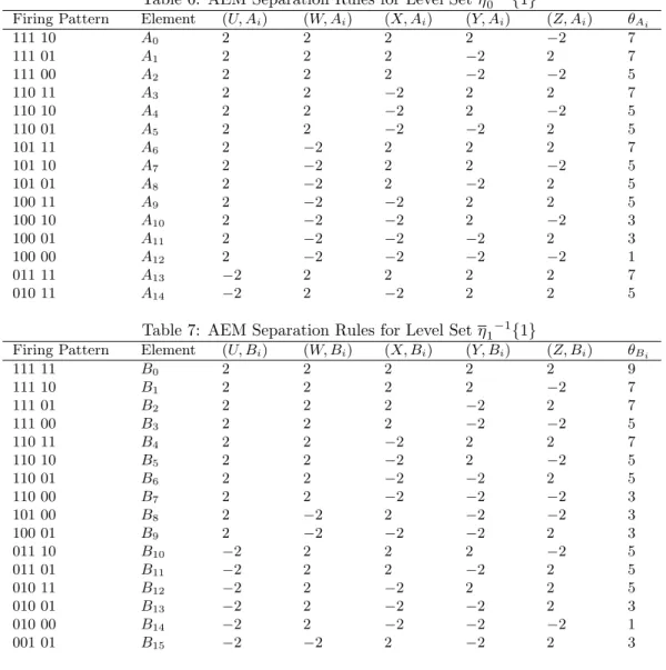
The level sets ofη_k :{0,1}3_{× {}₀_,₁_}2_{→ {}₀_,₁_}_where _k_{∈ {}₀_,₁_,₂_,₄_,₅_}_{are shown below.} η₀−1₍_{U W X, Y Z}_){1}₌_{(111_,₁₀₎_,₍₁₁₁_,₀₁₎_,₍₁₁₁_,₀₀₎_,₍₁₁₀_,₁₁₎_,₍₁₁₀_,₁₀₎_,₍₁₁₀_,₀₁₎_,₍₁₀₁_,₁₁₎_,₍₁₀₁_,₁₀₎_,₍₁₀₁_,₀₁₎ (100,11),(100,10),(100,01),(100,00),(011,11) (010,11)} η0−1(U W X, Y Z){0}={(111,11),(110,00),(101,00),(011,10),(011,01),(011,00),(010,10),(010,01),(010,00) (001,11),(001,10),(001,01),(001,00),(000,11),(000,10),(000,01),(000,00)} η1−1(U W X, Y Z){1}={(111,11),(111,10),(111,01),(111,00),(110,11),(110,10),(110,01),(110,00),(101,00) (100,01),(011,10),(011,01),(010,11),(010,01),(010,00),(001,01)} η1−1(U W X, Y Z){0}={(101,11),(101,10),(101,01),(100,11),(100,10),(100,00),(011,11),(011,00),(010,10) (001,11),(001,10),(001,00),(000,11),(000,10),(000,01),(000,00)} η2−1(U W X, Y Z){1}={(111,10),(111,01),(110,00),(101,11),(101,10),(101,01),(101,00),(100,01),(100,00) (011,10),(011,01),(010,10),(001,11),(001,10),(001,00)} η2−1(U W X, Y Z){0}={(111,11),(111,00),(110,11),(110,10),(110,01),(100,11),(100,10),(011,11),(011,00) (010,11),(010,01),(010,00),(001,01),(000,11),(000,10),(000,01),(000,00)} η4−1(U W X, Y Z){1}={(111,01),(110,11),(110,01),(110,00),(101,11),(101,01),(100,11),(100,01),(011,11) (011,01),(010,01),(001,11),(001,01)} η4−1(U W X, Y Z){0}={(111,11),(111,10),(111,00),(110,10),(101,10),(101,00),(100,10),(100,00),(011,10) (011,00),(010,11),(010,10),(010,00),(001,10),(001,00),(000,11),(000,10),(000,01),(000,00)} η5−1(U W X, Y Z){1}={(111,11),(111,10),(111,01),(111,00),(110,11),(110,10),(110,01),(101,11), (101,10) (101,01),(100,00),(010,11),(010,01),(010,00)} η5−1(U W X, Y Z){0}={(110,00),(101,00),(100,11),(100,10),(100,01),(011,11),(011,10),(011,01),(010,10) (001,11),(001,10),(001,01),(001,00),(000,11),(000,10),(000,01),(000,00)}

The level setη5−1(U W X, Y Z){h}={(011,00)} is the special case when the UTM halts (i.e.,

η(011,00) = (000,00, h) ). When the UTM halts, the AEM reaches a halting firing patternH. The next example copies one element’s firing state to another element’s firing state. This program helps assign the value of a random bit to an active element and perform other functions in the UTM. When the followingcopyprogram is called, active elementbfires ifafired during the window of time [s,t). Further, a connection is set up frombtobso thatbwill keep firing indefinitely. This enablesbto storeactive elementa’s firing state.

Example 2. Copy Program

An AEM program copies active elementa’s firing state to elementb. (Program copy (Args s t b a)

(Element (Time s-1) (Name b) (Threshold 1) (Refractory 1) (Last s-1)) (Connection (Time s-1) (From a) (To b) (Amp 0) (Width 0) (Delay 1)) (Connection (Time s) (From a) (To b) (Amp 2) (Width 1) (Delay 1)) (Connection (Time s) (From b) (To b) (Amp 2) (Width 1) (Delay 1)) (Connection (Time t) (From a) (To b) (Amp 0) (Width 0) (Delay 1)) )

Procedure 2. Computing Turing Programη with Random Firing Patterns Procedure 2 describes the computation ofη with random AEM firing patterns.

Consider function η3:{0,1}5→ {0,1}. The following scheme is used to represent boolean

values 1 and 0 with the firing of active elements. If active elementU fires during window W, then this corresponds to inputU = 1 inη₃; if active elementU doesn’t fire during windowW, then this corresponds to inputU = 0 in η₃. When U fires,W doesn’t fire, X fires,Y doesn’t fire andZ doesn’t fire, this corresponds to computingη₃(101,00). The value 1 =η₃(101,00) is the underlined bit in (011,10,0), which is located in row 101, column 00 of table 2.

Procedure 1 and the separation rules in table 3 are synthesized so thatη₃is computed using a dynamic interpretation determined by quantum random bits. This creates random active element firing patterns that computeη₃.

(10)

The firing activity of element P3 represents the output value of η3(U W X, Y Z). Fourteen

random bits are created from quantum randomness (See [42], [43]). These random bits create a corresponding random firing pattern of active elements R0, R1, . . . R13. Meta commands

dynamically build active elements and connections based on the separation rules in table 3 and the firing activity of elements R0, R1, . . . R13. These dynamically created elements and

connections determine the firing activity of elementP3based on the firing activity of elements

U, W, X, Y andZ. This procedure is described below.

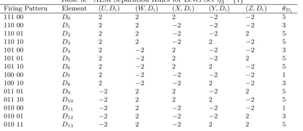
Table 3: AEM Separation Rules for Level Setη3−1{1}

Firing Pattern Element (U, Di) (W, Di) (X, Di) (Y, Di) (Z, Di) θDi

111 00 D0 2 2 2 −2 −2 5 110 00 D1 2 2 −2 −2 −2 3 110 01 D2 2 2 −2 −2 2 5 110 10 D3 2 2 −2 2 −2 5 101 00 D4 2 −2 2 −2 −2 3 101 01 D5 2 −2 2 −2 2 5 101 10 D6 2 −2 2 2 −2 5 100 00 D7 2 −2 −2 −2 −2 1 100 10 D8 2 −2 −2 2 −2 3 011 01 D9 −2 2 2 −2 2 5 011 10 D10 −2 2 2 2 −2 5 010 00 D11 −2 2 −2 −2 −2 1 010 01 D12 −2 2 −2 −2 2 3 010 11 D13 −2 2 −2 2 2 5

Step 2.1 A quantum source creates fourteen random bitsa0,a1,. . . anda13. These bit

values are stored in elementsR0,R1, . . . , R13. If ak = 1, then Rk fires; if ak = 0, Rk doesn’t

fire.

Step 2.2 Set up dynamical connections from active elements U, X, W, Y, Z to elements D0, D1, . . . , D13, which depend on meta commands that use the firing pattern from elements

R0, R1, . . . R13.

ForD0, look at the first row and first column of table 3. The firing pattern 111 00 means

thatD0 dynamically separates this pattern with respect to the other firing patterns ofU W X

Y Z. The separation is dynamic based on whether elementR0 fires or doesn’t fire. IfR0fires,

then D0 fires when the firing pattern for U W X Y Z is 111 00; for all other firing patterns

for U W X Y Z, then D0 doesn’t fire. If R0 doesn’t fire, then D0 doesn’t fire when the firing

pattern for U W X Y Z is 111 00; for all other firing patterns for U W X Y Z, then D0 fires.

In a similar way, D1 dynamically separates the firing pattern 110 00 for U W X Y Z based on

whether elementR1 fires. Observe that every firing pattern in the first column is in the level

set ofη₃−1_{₁_}_.

The firing pattern 111 00 corresponds to theηinstruction (111,00), whose output (110,10,1)

is shown in the last row and second column of table 2. The amplitudes from U, W, X, Y, Z to

D0are labeled by the headers (U, Di), (W, Di), (X, Di), (Y, Di) and (Z, Di), respectively. D0’s

threshold 5 is in the first row under the headerθDi.

(Program set_dynamic_C (Args s t f xk a w tau rk)

(Connection (Time s-dT) (From f) (To xk) (Amp -a) (Width w) (Delay tau)) (Meta (Name rk) (Window s t)

(11)

(Program set_dynamic_E (Args s t xk h r L rk)

(Element (Time s-2dT) (Name xk) (Threshold -h) (Refractory r) (Last L)) (Meta (Name rk) (Window s t)

(Element (Time t) (Name xk) (Threshold h) (Refractory r) (Last L))) )

(set_dynamic_E (Args s t D0 5 1 s-2 R0)) (set_dynamic_C (Args s t U D0 2 1 1 R0)) (set_dynamic_C (Args s t W D0 2 1 1 R0)) (set_dynamic_C (Args s t X D0 2 1 1 R0)) (set_dynamic_C (Args s t Y D0 -2 1 1 R0)) (set_dynamic_C (Args s t Z D0 -2 1 1 R0))

At times-dT,set_dynamic_Cinitializes the amplitudes of the connections toAU D0 =−2,

AW D0 = −2, AXD0 = −2, AY D0 = 2, AZD0 = 2. If R0 fires, then the meta command in

set_dynamic_C, causes the connection command to execute at time t, which flips the sign of each of the amplitudes to AU D0 = 2, AW D0 = 2, AXD0 = 2, AY D0 = −2, AZD0 = −2.

Similarly, set_dynamic_E initializes the threshold ofD0 to θD0 = −5. If R0 fires, then the

meta command causes the element command to execute at timet, which flips the sign of the

threshold ofD0. In this case,θD0= 5.

Similarly, for elements D1, . . . , D13, set_dynamic_E and set_dynamic_C dynamically set

the element parameters and the connections fromU, X, W, Y, Z to D1, . . . , D13 based on the

rest of the quantum random firing pattern R1, . . . R13 and the appropriate parameter values

shown in table 3.

Step 2.3 Set up connections to active elementsG0, G1, G2, . . . G14 which represent the

number of elements in{R0, R1, R2, . . . R13}that are firing. If 0 are firing, then onlyG0is firing.

Otherwise, ifk >0 elements in{R0, R1, R2, . . . R13} are firing, then onlyG1, G2, G3. . . Gk are

firing.

(Program firing_count (Args G a b h)

(Element (Time a-2dT) (Name G) (Threshold h) (Refractory b-a) (Last 2a-b)) (Connection (Time a-dT) (From R0) (To G) (Amp 2) (Width b-a) (Delay 1)) (Connection (Time a-dT) (From R1) (To G) (Amp 2) (Width b-a) (Delay 1))

. . .

(Connection (Time a-dT) (From R13) (To G) (Amp 2) (Width b-a) (Delay 1)) )

(firing_count (Args G0 a b -1)) (firing_count (Args G1 a b 1)) . . . (firing_count (Args G13 a b 25)) (firing_count (Args G14 a b 27))

Step 2.4 Element P3 represents the output of η3. Initialize P3’s threshold based on

meta commands that use the firing activity from elementsG0, G1, G2, . . . G13. Sincet + dT<

t + 2dT <· · · < t + 15dT, the meta commands set the threshold for P3 to −2(14−k) + 1

where k is the number of firings. For example, if nine of the randomly chosen bits are high,

thenG9 will fire, so the threshold ofP3 is set to−9. If five of the random bits are high, then

the threshold ofP3is set to−17. Each element of the level setη3−1{0}creates a firing pattern

ofD0, . . . D13 equal to the complement of the random firing patternR0R1. . . R13 (i.e.,Dk fires

if and only ifRk does not fire).

(Program set_P_threshold (Args G P s t a b theta kdT) (Meta (Name G) (Window s t)

(Element (Time t+kdT) (Name P) (Threshold theta) (Refractory b-a) (Last t-b+a))))

(set_P_threshold (Args G0 P3 s t a b -27 dT)) (set_P_threshold (Args G1 P3 s t a b -25 2dT))

(12)

. . .

(set_P_threshold (Args G13 P3 s t a b -1 14dT)) (set_P_threshold (Args G14 P3 s t a b 1 15dT))

Step 2.5 Set up dynamical connections from D0, D1, D2, . . . , D13 to P3 based on the

random bits stored by R0, R1, . . . R13. These connections are based on meta commands that

use the firing pattern from elementsR0, R1, . . . R13.

(Program set_from_Xk_to_Pj (Args s t Xk Pj a w tau Rk)

(Connection (Time s-dT) (From Xk) (To Pj) (Amp -a) (Width w) (Delay tau)) (Meta (Name Rk) (Window s t)

(Connection (Time t) (From Xk) (To Pj) (Amp a) (Width w) (Delay tau))) )

(set_from_Xk_to_Pj (Args s t D0 P3 2 b-a 1 R0)) . . . (set_from_Xk_to_Pj (Args s t D13 P3 2 b-a 1 R13))

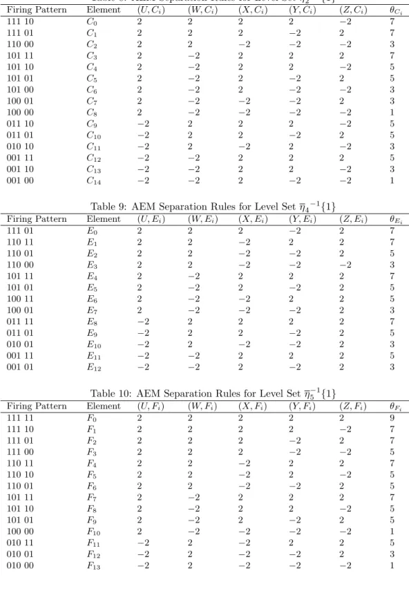
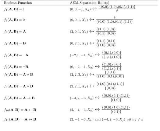
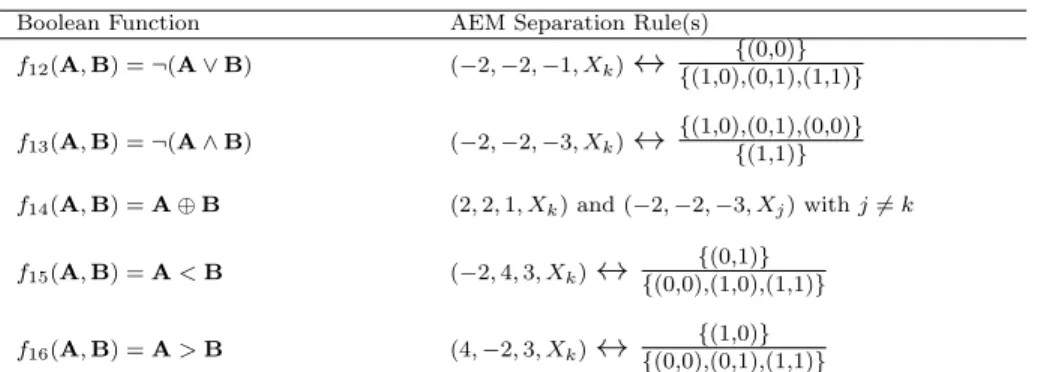
Similar procedures use random firing patterns on elements {A0, . . . , A14}, {B0, . . . , B15}, {C0, . . . , C14},{E0, . . . , E12}, and{F0, . . . , F13}to computeη0,η1,η2,η4, andη5, respectively.

The outputs ofη₀,η₁,η₂,η₄, andη₅ are represented by active elementsP0, P1, P2, P4 andP5,

respectively. In subsection 7.5 of the appendix, the level set rules forη₀,η₁,η₂,η₄, andη₅are shown, respectively in tables 6, 7, 8, 9 and 10.

The firing activity of elementPk represents a single bit that helps determine the next state

or next tape symbol during a UTM computational step. If an eavesdropper is able to listen to the firing activity ofP0, P1, P2, P3, P4 andP5, which collectively represent the computation of

η(U XW, Y Z), then this leaking of information could be used to reconstruct some or all of the UTM tape contents. This weakness can be rectified as follows. For each UTM computational step, the AEM uses six additional quantum random bitsb0, b1, b2, b3, b4, b5. ForP3, if random

bitb3= 1, then the dynamical connections fromD0, D1, . . . D13 toP3are chosen as described

above. However, if random bitb3= 0, then the amplitudes of the dynamical connections from

D0, D1, . . . D13 toP3and the threshold ofP3are multiplied by−1. This causesP3to fire when

η₃(U XW, Y Z) = 0 andP3 doesn’t fire whenη3(U XW, Y Z) = 1.

This cloaking of P3’s firing activity can be coordinated with a meta command based on

the value ofb3so thatP3’s firing is appropriately interpreted to dynamically change the active

elements and connections that update the UTM tape contents and state after each computa-tional step. This cloaking procedure can also be used for elementPk and random bitbk where k∈ {0,1,2,4,5}. Furthermore, the same methods can be used to cloak the active element firing patterns that represent the UTM’s state and tape contents. In particular, these methods may help cloak the firing pattern representing the halting stateH.

Besides representing and computing the programη with quantum random firing patterns,

there are other useful functions computed by active elements executing the UTM. Assume that these connections and the active element firing activity are kept perfectly secret as they represent the state and the tape contents of the UTM tape contents. Alternatively, the active elements representing the UTM tape contents and state may be cloaked similar to the description for cloaking elementsP0, P1, . . . , P5.

• Three active elements (q 0), (q1) and (q2) store the current state of the UTM.

• There are a collection of elements to represent the tape head location k where k is an

(13)

• A marker active elementLlocates the leftmost tape square and a separate marker active

element R locates the rightmost tape square. Any tape symbols outside these markers

are assumed to be blank (i.e., 0). If the tape head moves beyond the leftmost tape

square, thenL’s connection is removed and updated one tape square to the left and the

machine is reading a 0. If the tape head moves beyond the rightmost tape square, then

R’s connection is removed and updated one tape square to the right and the machine is

reading a 0.

• There are a collection of elements that represent the tape contents of the UTM. For each

tape squarekinside the marker elements, there are two elements named (S k) and (T k)

whose firing pattern determines the alphabet symbol at tape square k. For example, if

elements (S 5) and (T 5) are not firing, then tape square 5 contains alphabet symbol 0. If element (S −7) is firing and element (T −7) is not firing, then tape square−7 contains alphabet symboly. If element (S−4) is not firing and element (T −4) is firing, then tape

square −4 contains alphabet symbol 1. If elements (S 13) and (T 13) are both firing,

then tape square 13 contains alphabet symbolA.

• Representing alphabet symbol 0 with two active elements that are not firing is convenient because if the tape head moves beyond the initial tape contents of the UTM, then the meta command can add two elements that are not firing to represent the contents of the new square.

The copy program helps construct useful functionality in the UTM. The following program helps copy a new alphabet symbol to the tape.

(Program copy_symbol (Args s t b0 a0 b1 a1)

(copy (Args s t b0 a0)) (copy (Args s t b1 a1)) ) The following program enables a new state to be copied. (Program copy_state (Args s t b0 a0 b1 a1 b2 a2)

(copy (Args s t b0 a0)) (copy (Args s t b1 a1)) (copy (Args s t b2 a2)) )

The sequence of steps by which the UTM is executed with an AEM are described below. 1. Tape contents are initialized and the marker elementsLandRare initialized.

2. The tape head is initialized to tape squarek= 0 and the current machine state is initial-ized toq2. In other words, (q0) is not firing (q1) is firing and (q2) is not firing.

3. (S k) and (T k) are copied toainand the current state (q0), (q1), (q2) is copied toqin.

andmrepresents the tape head move.

4. Ifqout=H, then the UTM halts: the AEM reaches a firing pattern that stores the current

tape contents indefinitely and keeps the tape head fixed at tape squarekwhere the UTM

halted.

5. Otherwise, the firing pattern of the three elements representing qout are copied to (q 0),

(q1), (q 2). aout is copied to the current tape square represented by (S k), (T k).

6. Ifm=L, then first determine if the tape head has moved to the left of the tape square

marked byL. If so, then haveLremove its current marker and mark tape squarek−1.

(14)

7. Ifm=R, then first determine if the tape head has moved to the right of the tape square

marked byR. If so, then haveRremove its current marker and mark tape squarek+ 1.

In either case, go back to step 3 where (S k+ 1) and (T k+ 1) are copied toain.

First, a simple lemma is proved. This lemma will help show that for a non-halting

UTM computation the firing activity of the elements computing η (i.e.,{A0, . . . , A14, P0}, {B0, . . . , B15, P1},{C0, . . . , C14, P2},{D0, . . . , D13, P3},{E0, . . . , E12, P4}and{F0, . . . , F13, P5}

) is incomputable.

Lemma 4.1. Let γ:_N→ {0,1}be an incomputable function. For eachk such that1≤k≤m assume the boolean function Bk : {0,1}n → {0,1}n is invertible. Let h : N → {1, . . . , m}

be a computable function. Define function g : _N → {0,1} where (g(1), g(2), . . . , g(n)) = Bh(1)(γ(1), γ(2), . . . , γ(n)) and where (g(n+ 1), g(n + 2), . . . , g(2n)) = Bh(2)(γ(n + 1),

γ(n+ 2), . . . , γ(2n)), and for thejthn-tuple in {0,1}n ₍_g₍_jn_{+ 1)}_{, g}₍_jn_{+ 2)}_{, . . . , g}₍₍_j_{+ 1)}_n₎₎

=Bh(j)(γ(jn+ 1), γ(jn+ 2), . . . , γ((j+ 1)n)),. . .. Theng is an incomputable function.

Proof. By reductio ad absurdum, supposegis a computable function. Theng(1), g(2), . . . , g(m) are computable. Since h(1) is computable and each Bk is invertible and boolean, B_h−₍₁₎1 is

computable. ThenB_h−₍₁₎1 (g(1), g(2), . . . , g(n)) is computable which equals (γ(1), . . . , γ(n)). This

completes the base case that γ is computable. Repeating this computation j −1 times, by

induction,γ(1), . . . , γ((j−1)n) are computable. For the inductive step, g(jn+ 1), g(jn+ 2), . . . , g((j+ 1)n) is computable. Since h(j) is computable, then B_h−₍1_j₎ is computable. Thus, B_h−₍1_j₎(g(jn+ 1), g(jn+ 2), . . . , g((j+ 1)n)) is computable which equals (γ(jn+ 1), γ(jn+ 2), . . . , γ((j + 1)n)). The induction principle implies that γ(i) is computable for every natural numberiwhich is a contradiction.

Definition 3. Representing the firing activity of the active elements computingη

Consider the jth computational step of the UTM. Fork such that 1≤k≤15, letfk,j = 1

if elementAk−1 fires during thisjth step andfk,j = 0, otherwise. Letf16,j represent the firing

activity ofP0. For k such that 17 ≤ k ≤ 32, let fk,j = 1 if element Bk−17 fires during this

jth step andfk,j = 0, otherwise. Let f33,j represent the firing activity ofP1. Fork such that

34≤k≤48, let fk,j = 1 if elementCk−34 fires during this jth step andfk,j = 0, otherwise.

Letf49,j represent the firing activity ofP2. Forksuch that 50≤k≤63, letfk,j = 1 if element Dk−50 fires during thisjth step andfk,j = 0, otherwise. Letf64,j represent the firing activity

ofP3. Forksuch that 65≤k≤77, letfk,j = 1 if elementEk−65 fires during thisjth step and

fk,j = 0, otherwise. Letf78,j represent the firing activity ofP4. Forksuch that 79≤k≤92, let

fk,j = 1 if elementFk−79 fires during thisjth step andfk,j = 0, otherwise. Letf93,j represent

the firing activity ofP5.

Definition 4. Unbounded number of computable UTM steps

If the UTM execution does not halt, then fk,j is defined for every natural number j. If

the UTM execution halts on a finite or infinite number of tape inputs, then the definition of f1,j, . . . , f93,j can be extended as follows. Suppose the first tape input halts after m1 steps.

Before the second UTM execution starts, it is assumed that the UTM’s tape contents are initialized using a computable method. For the first computational step,j=m1+1. Inductively,

(15)

are initialized using a computable method. On the first step of the k+ 1th UTM execution j=m1+m2+. . . mk+ 1.

For an unbounded number of computable UTM steps, define the function g : N→ {0,1}

whereg(93(j−1)+r+1) =f(r+1),j and 0≤r <93. In other words,g(1) =g(93(1−1)+1) =f1,1 g(2) =f2,1 . . . g(93) =f93,1 g(94) =f1,2 and so on.

Theorem 4.2. If an unbounded number of computable UTM steps are executed by the AEM according to Procedure 2 and the two quantum randomness axioms hold, theng is an incom-putable function.

Proof. It suffices to show that the sequence (f1,1, f2,1, . . . f93,1, f1,2, f2,2, . . . , f93,2, . . . , f1,j, . . . f93,j, . . .) in Ω is Turing incomputable. The proof covers the computation of η3.

Simi-lar steps, described below, can be verified forη₀, η₁, η₂, η₄ and η₅. Lemma 4.1 is applied and the proof is completed.

The function γin 4.1 is defined based on the firing activity of R0, R1, . . . , R13 discussed in

steps 2.1 and 2.2 and quantum random bitb3. From [4], the two quantum randomness axioms

imply that γ is Turing incomputable. (Alternatively, it can be shown that the two quantum

randomness axioms induce a Lebesgue probability measure on Ω. The computable sequences in Ω have Lebesgue measure zero because they are countable. Thus, any infinite quantum random sequence is incomputable with probability = 1).

From definition 3, g represents the firing activity of elements A0, . . . , A14, B0, . . . , B15,

C0, . . . , C14, D0, . . . , D13, E0, . . . , E12, F0, . . . , F13and of output elementsP0, P1, P2, P3, P4, P5. g corresponds to function g in lemma 4.1. The elements D0, . . . , D13 are discussed in steps

2.1 and 2.2. For each computational step of the UTM, table 4 shows how the AEM maps the firing activity of R0, R1, . . . , R13, b3 to the firing activity of D0, D1, . . . , D13, P3. This is

verified by checking the program definitions ofset_dynamic_Candset_dynamic_Ein step 2.2.

For example, if the current UTM instruction is (111,00) – i.e., in state 111 and reading tape symbol 00 – then this corresponds to boolean functionB(111,00)shown in the first row of table 4.

B(111,00)defines the mapping ofR0, R1, . . . , R13, b3to the firing activity ofD0, D1, . . . , D13, P3.

Each boolean functionBk in table 4 is invertible becauseBk◦Bk equals the identity.

The final verification is that h : N → {1,2, . . . ,15} is computable. First, identify 1 with

instruction (111,00), 2 with instruction (110,00),. . ., 14 with instruction (010,11) and 15 with η3−1{0}. Let (q, Tk) be the current state and tape symbol of the UTM at thejth computational

step. Defineh(j) = (q, Tk) ifη3(q, Tk) = 1. Otherwise, defineh(j) =η3−1{0}. Sincehcan be

computed based on the computation of the UTM,h is computable. In the other case, where

the UTM execution halts one or more times, definition 4 assumes that the initialization of the

UTM tape contents is computable, sohis computable.

Theorem 4.3. If an adversary can only eavesdrop on the firing activity of (f1,1, f2,1, . . . f93,1,

. . . , f1,j, . . . f93,j, . . .)then the AEM execution, described in Procedure 2, of the UTM is perfectly

secret. In other words, P(q =qk) =P(q =qk | f1,j =b1 . . . fm,j =bm) andP(Tk =ak) = P(Tk =ak | f1,j =b1 . . . fm,j =bm) for eachbi ∈ {0,1}, where q is the current state of the

UTM andTk is the contents of thekth tape square.

Proof. The proof is a straightforward consequence of the two quantum randomness axioms, the boolean functions in table 4 characterizing the firing activity off1,1. . . , f1,j, . . . f93,j, . . . and

the definition of conditional probability.

Let event Q correspond to q = qk. Let event B correspond to f1,j = b1. Then event

(16)

Table 4: Boolean functions Bk:{0,1}15→ {0,1}15forη3

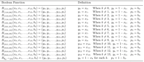
Boolean Function Definition

B(111,00)(x0, x1, . . . , x13, b3) = (y0, y1, . . . , y13, p3) y0=x0. Whenk6= 0, yk= 1−xk. p3=b3. B(110,00)(x0, x1, . . . , x13, b3) = (y0, y1, . . . , y13, p3) y1=x1. Whenk6= 1, yk= 1−xk. p3=b3. B(110,01)(x0, x1, . . . , x13, b3) = (y0, y1, . . . , y13, p3) y2=x2. Whenk6= 2, yk= 1−xk. p3=b3. B(110,10)(x0, x1, . . . , x13, b3) = (y0, y1, . . . , y13, p3) y3=x3. Whenk6= 3, yk= 1−xk. p3=b3. B(101,00)(x0, x1, . . . , x13, b3) = (y0, y1, . . . , y13, p3) y4=x4. Whenk6= 4, yk= 1−xk. p3=b3. B(101,01)(x0, x1, . . . , x13, b3) = (y0, y1, . . . , y13, p3) y5=x5. Whenk6= 5, yk= 1−xk. p3=b3. B(101,10)(x0, x1, . . . , x13, b3) = (y0, y1, . . . , y13, p3) y6=x6. Whenk6= 6, yk= 1−xk. p3=b3. B(100,00)(x0, x1, . . . , x13, b3) = (y0, y1, . . . , y13, p3) y7=x7. Whenk6= 7, yk= 1−xk. p3=b3. B(100,10)(x0, x1, . . . , x13, b3) = (y0, y1, . . . , y13, p3) y8=x8. Whenk6= 8, yk= 1−xk. p3=b3. B(011,01)(x0, x1, . . . , x13, b3) = (y0, y1, . . . , y13, p3) y9=x9. Whenk6= 9, yk= 1−xk. p3=b3. B(011,10)(x0, x1, . . . , x13, b3) = (y0, y1, . . . , y13, p3) y10=x10. Whenk6= 10, yk= 1−xk. p3=b3. B(010,00)(x0, x1, . . . , x13, b3) = (y0, y1, . . . , y13, p3) y11=x11. Whenk6= 11, yk= 1−xk. p3=b3. B(010,01)(x0, x1, . . . , x13, b3) = (y0, y1, . . . , y13, p3) y12=x12. Whenk6= 12, yk= 1−xk. p3=b3. B(010,11)(x0, x1, . . . , x13, b3) = (y0, y1, . . . , y13, p3) y13=x13. Whenk6= 13, yk= 1−xk. p3=b3. Bη3−1{0}(x0, x1, . . . , x13, b3) = (y0, y1, . . . , y13, p3) yk= 1−xk for eachk. p3= 1−b3. xk= 1 if elementRkfires. Ifb3= 1, P3fires iff (U W X, Y Z)∈η3

−1

{1}.

xk= 0 if elementRkdoesn’t fire. Ifb3= 0, P3fires iff (U W X, Y Z)∈η3

−1

{0}.

=P(Rk = 1) =P(B) =P(B) = 1₂ and from the properties of the boolean functions in table 4.

Thus, P(Q) =P(Q | B) which means that P(q =qk) = P(q =qk | f1,j =b1). Similar steps

can be repeated to show thatP(q=qk) =P(q=qk |f1,j =b1. . . fm,j =bm) andP(Tk=ak)

=P(Tk=ak |f1,j =b1 . . . fm,j=bm).

It is worth mentioning that if the system reveals information about the dynamic connections fromRktoDk or the quantum random bits generated or firing activity of elementsRkor those

elements representing the UTM tape or state, then the perfect secrecy doesn’t hold.

Corollary 1. Consider an unbounded number of computable steps generated by the AEM in procedure 2, where the sequence of UTM instructions isI1, I2, . . . , Ik, . . ., and Ik ∈Q× A as

defined in table 2. Define function f : N → Q× A as f(k) = Ik. If an adversary can only

eavesdrop on g (the firing activity computing η), then there does not exist a Turing machine that can mapgback to f.

Proof. This corollary follows from definition 1 and the work in lemma 4.1 and theorems 4.2 and 4.3.

5 Summary

By using a finite AEM program and the meta command, and executing procedure 2, any Turing machine program – with a computable unbounded execution – can be executed with AEM firing patterns that are Turing incomputable. For an unbounded number of computable UTM execution steps, when appropriate parameters of the AEM execution are not revealed to an adversary, then there does not exist a Turing machine that can mapg(i.e., the active element

(17)

firing patterns computing η) back to the sequence of universal Turing machine instructions executed by the AEM.

6 Acknowledgements

I would like to thank Wolfgang Halang, Michael Jones, Don Knuth, David Lewis, A. Mayer, Lutz Mueller, Don Saari and Mario Stip˘cevi´c for their helpful advice.

References

[1] P. Benioff. The computer as a physical system: A microscopic quantum mechanical Hamiltonian model of computers as represented by Turing machines.Journal of Statistical Physics, 22:563–591, 1980.

[2] P. Benioff. Quantum mechanical Hamiltonian models of Turing machines that dissipate no energy. Physics Review Letter, 48:1581–1585, 1980.

[3] Cristian S. Calude, Michael J. Dinneen, Monica Dumitrescu, and Karl Svozil. Experimental Evidence of Quantum Randomness Incomputability. Physics Review A, 82(022102):1–8, 2010. [4] Cristian S. Calude and Karl Svozil. Quantum randomness and value indefiniteness. Advanced

Science Letters, 1(2):165–168, 2008.

[5] Alonzo Church. An Unsolvable Problem of Elementary Number Theory. American Journal of Mathematics, 58:345–363, 1936.

[6] Fred Cohen. Computer Viruses Theory and Experiments. Computers and Security, 6(1):22–35, February 1987.

[7] S. Barry Cooper. The Incomputable Alan Turing. InTuring 2004: A celebration of his life and achievements. Electronic Workshops in Computing, June 2004.

[8] S. Barry Cooper and Piergiorgio Odifreddi. Incomputability in Nature. Plenum Publishers, 2003. [9] Martin Davis. Computability and Unsolvability. Dover Publications, 1982.

[10] Martin Davis. The Myth of Hypercomputation. Springer-Verlag, 2004.

[11] Martin Davis. Why there is no such discipline as hypercomputation. Applied Mathematics and Computation, 178(1):4–7, July 2006.

[12] K. de Leeuw, E.F. Moore, C.E. Shannon, and N. Shapiro.Computability of Probabilistic Machines. Princeton University Press, 1956.

[13] David Deutsch. Quantum theory, the Church-Turing principle and the universal quantum com-puter. Proceedings of London Mathematical Society. Series A, 400(1818):97–117, 1985.

[14] Gábor Etesi and István Németi. Non-Turing computations via Malament-Hogarth spacetimes. International Journal of Theoretical Physics, 41(2):341–370, 2002.

[15] Richard Feynman. Simulating physics with computers. International Journal of Theoretical Physics, 21:467–488, 1982.

[16] Richard Feynman. Quantum mechanical computers. Foundations of Physics, 16:507–531, 1986. [17] Eric Filiol.Malicious Cryptology and Mathematics. Intech, 2012.

[18] Michael Stephen Fiske. The Active Element Machine. InProceedings of Computational Intelli-gence. Autonomous Systems: Developments and Trends, volume 391, pages 69–96. Springer-Verlag, 2011.

[19] L.K. Grover. Quantum mechanics helps in searching for a needle in a haystack. Physics Review Letters, 79:325–328, 1997.

[20] Wolfgang Halang and Boudewijn Hoogeboom.The concept of time in the specification of real-time systems. Kluwer Academic Publishers, 1992.

(18)

[21] John Hertz, Anders Krogh, and Richard G. Palmer. Introduction To The Theory of Neural Com-putation. Addison-Wesley, Redwood City, California, 1991.

[22] Mark Hogarth. Does general relativity allow an observer to view an eternity in a finite time? Foundations of Physics Letters, 5(2):173 – 181, 1992.

[23] Mark Hogarth. Non-Turing Computers and Non-Turing Computability. In Proceedings of the Biennial Meeting of the Philosophy of Science Association, volume 1, pages 126 – 138. University of Chicago Press, 1994.

[24] John J. Hopfield. Neural networks and physical systems with emergent collective computational abilities. Proceedings of the National Academy of Sciences, 79:2554 – 2558, 1982.

[25] John J. Hopfield. Pattern recognition computation using action potential timing for stimulus representation.Nature, 376:33 – 36, 1995.

[26] John J. Hopfield and D.W. Tank. Neural computation of decisions in optimization problems. Biological Cybernetics, 52:141 – 152, 1985.

[27] Tien Kieu. Quantum Algorithm for Hilbert’s Tenth Problem.http://arxiv.org/abs/quant-ph/ 0110136, 2001.

[28] Paul Kocher, Joshua Jaffe, and Benjamin Jun. Differential Power Analysis. In Advances in Cryptology - Crypto 99 Proceedings. Lecture Notes in Computer Science, volume 1666. Springer-Verlag, 1999.

[29] Harry R. Lewis and Christos H. Papadimitriou. Elements Of The Theory Of Computation. Prentice-Hall, 1981.

[30] Yuri Manin. A Course in Mathematical Logic. Springer-Verlag, 1977.

[31] Yuri Manin. Computable and Uncomputable (in Russian). Sovetskoye Radio, Moscow, 1980. [32] Warren S. McCulloch and Walter Pitts. A logical calculus immanent in nervous activity.Bulletin

of Mathematical Biophysics, 5:115 – 133, 1943.

[33] Marvin Minsky. Computation: Finite and Infinite Machines. Prentice-Hall (1st edition), Engle-wood Cliffs, New Jersey, 1967.

[34] Marvin Minsky and Seymour A. Papert. Perceptrons. MIT Press, Cambridge, Massachusetts, 1969.

[35] Wilfrid Rall. The Theoretical Foundation of Dendritic Function. Selected Papers of Wilfrid Rall with Commentaries. Edited by Idan Segev, John Rinzel, and Gordon Shepherd. MIT Press, Cam-bridge, Massachusetts, 1995.

[36] Abraham Robinson.Non-standard Analysis. Princeton University Press (Revised Edition), Prince-ton, New Jersey, 1996.

[37] Frank Rosenblatt. Two theorems of statistical separability in the perceptron. In Proceedings of a Symposium on the Mechanization of Thought Processes, pages 421 – 456, London, 1959. Her Majesty’s Stationary Office.

[38] Claude Shannon. Communication Theory of Secrecy Systems. http://netlab.cs.ucla.edu/ wiki/files/shannon1949.pdf, 1949.

[39] Peter W. Shor. Algorithms for quantum computation: discrete log and factoring. InProceedings of the 35th Annual IEEE Symposium on Foundations of Computer Science, pages 2 – 22, 1994. [40] Hava Siegelmann. Computation Beyond the Turing Limit. Science, 268(5210):545 – 548, April

1995.

[41] Robert Soare. Computability and Recursion. Bulletin of Symbolic Logic, 2:284 – 321, 1996. [42] Andr´e Stefanov, Nicolas Gisin, Olivier Guinnard, Laurent Guinnard, and Hugo Zbinden. Optical

quantum random number generator. Journal of Modern Optics, 47(4):595 – 598, 2000.

[43] Mario Stip˘cevi´c and B. Medved Rogina. Quantum random number generator based on photonic emission in semiconductors. Review of Scientific Instruments, 78:1 – 7, 2007.

(19)

Computing Machines, 10:217–255, 1963.

[45] Alan M. Turing. On Computable Numbers, with an Application to the Entscheidungsproblem. Proceedings of the London Mathematical Society. Series 2, 42(3 and 4):230–265, 1936.

7 Appendix

7.1 Turing Machine

Define a Turing Machine, where the program definitionηis explicitly represented as a function instead of quintuples ([9], [45]).

Definition 5. Turing Machine

A Turing machine is a triple (Q,A, η) where

• Qis a finite set of states that does not contain a unique halting state, represented asH.

• When machine execution begins, the machine is in an initial statesands∈Q.

• Ais a finite set of alphabet symbols that are read from and written to the tape. • LandR represent advancing the tape head to the left or right square, respectively.

• η is a function where η : Q× A → Q× A × {L, R} ∪ {H} × A × {h}. η acts as the

programfor the Turing machine. For eachqinQandαinA,η(q, α) = (r, β, x) describes

how machine (Q,A, η) executes one computational step. When in stateq and scanning

alphabet symbolαon the tape:

– Machine (Q,A, η) changes to stater.

– Machine (Q,A, η) rewrites alphabet symbolαas symbolβ on the tape.

– Ifx=L, then machine (Q,A, η) moves its tape head one square to the left on the tape and is subsequently scanning the symbol in this square.

– Ifx=R, then machine (Q,A, η) moves its tape head one square to the right on the tape and is subsequently scanning the symbol in this square.

– If x=h, machine (Q,A, η) enters the halting stateHand the machine stops exe-cuting.

Definition 6. Turing Machine Tape

The Turing machine tapeT is represented as a functionT :Z→ AwhereZis the integers.

The tapeT isM-bounded if there exists a bound M >0 such that T(k) =T(j) whenever |k|,|j| ≥ M. The Turing machine definitions in [9] and [45] assume the initial tape, before

program execution begins, is M-bounded and the tape contains only blank symbols, denoted

here as #, outside the bound. The symbol on thekth square of the tape isT(k).

Definition 7. Configuration with Tape Head Location

Let (Q,A, η) be a Turing machine with tape T. A configuration is an element of the set

C = (Q∪ {H})×Z× {T : T is tape with range A}. If (q, k, T) is a configuration, then k is

(20)

Consider the configuration (p,2, . . .##αβ##. . .). The 1st coordinate indicates that the

Turing machine is in state p. The 2nd coordinate indicates that its tape head is currently

scanning tape square 2, denoted as T(2). The 3rd coordinate indicates that tape square 1

contains symbolα, tape square 2 contains symbolβ, and all other tape squares contain the # symbol. The underlining ofβ indicates that the tape head is currently scanning tape square 2.

Definition 8. Turing Machine Computational Step

Given Turing machine (Q,A, η) in current configuration (q, k, T) such thatT(k) =α. After the execution of one computational step, the new configuration is determined by one and only one of the three cases.

1. (r, k−1, S) if η(q, α) = (r, β, L) for non-halting stater. 2. (r, k+ 1, S) if η(q, α) = (r, β, R) for non-halting stater. 3. (H, k, T) if η(q, α) = (H, α, h) for halting stateH.

In cases (1) and (2) the new tapeS(j) =T(j) wheneverj6=kand S(k) =β. In case (3) the machine execution halts. Sometimes (q, α) is called a Turing machine instruction.

If the machine is currently in configuration (q0, k0, T0) and over the nextnsteps the sequence

of machine configurations (points) is (q0, k0, T0), (q1, k1, T1), (q2, k2, T2), . . . ,(qn, kn, Tn), then

this execution sequence is sometimes called the nextncomputational steps.

Table 5: Minsky Universal Turing Machine with Programη from [33]

y 0 1 A q1 (q1, 0,L) (q1, 0,L) (q2, 1,L) (q1, 1,L) q2 (q1, 0,L) (q2,y,R) (q2,A, R) (q6,y,R) q3 (q3,y,L) (H, 0,h) (q3,A, L) (q4, 1,L) q4 (q4,y,L) (q5,y,R) (q7, 1,L) (q4, 1,L) q5 (q5,y,R) (q3,y,L) (q5,A, R) (q5, 1,R) q6 (q6,y,R) (q3,A,L) (q6,A, R) (q6, 1,R) q7 (q7, 0,R) (q6,y,R) (q7, 1,R) (q2, 0,R)

State setQ={q1, q2, q3, q4, q5, q6, q7}. Alphabet A={y,0,1, A}. Halt stateH.

7.2 Active Element Machine Architecture

Define the extended integers asZ={m+kdT :m, k∈ZanddT is a fixed infinitesimal}. For

more on infinitesimals, see keyword 1 and reference [36].

Definition 9. Machine Architecture

Γ,Ω, and∆are index sets that index the input, computational, and output active elements, respectively. Depending on the machine architecture, the intersectionsΓ∩ΩandΩ∩∆can be empty or non-empty. A machine architecture, denoted as M(I,E,O), consists of a collection of input active elements, denoted as I = {Ei : i ∈ Γ}; a collection of computational active

elementsE ={Ei:i∈Ω}; and a collection of output active elements O={Ei:i∈∆}.

Each computational and output active element,Ei, has the following components and

(21)

• A thresholdθi

• A refractory periodri whereri>0.

• A collection of pulse amplitudes{Aki:k∈Γ∪Ω}.

• A collection of transmission times{τki:k∈Γ∪Ω}, whereτki>0 for all k∈Γ∪Ω.

• A function of time, Ψi(t), representing the time active element Ei last fired. Ψi(t) =

sup{s:s < tandgi(s) = 1}, wheregi(s) is the output function of active elementEi and

is defined below. The sup is the least upper bound and is always defined here, whence Ψi

is well-defined.

• A binary output function, gi(t), representing whether active elementEi fires at time t.

The value of gi(t) = 1 if PAki(t) > θi where the sum ranges over all k ∈ Γ∪Ω and t≥Ψi(t) +ri. In all other cases,gi(t) = 0. For example,gi(t) = 0, ift <Ψi(t) +ri.

• A set of firing times of active elementEk within active elementEi’s integrating window, Wki(t) ={s: active elementEk fired at times and 0≤t−s−τki< ωki}. Let |Wki(t)|

denote the number of elements in the setWki(t). IfWki(t) =∅, then|Wki(t)|= 0.

• A collection of input functions, {φki : k ∈ Γ∪Ω}, each a function of time, and each

representing pulses coming from computational active elements, and input active elements. The value of the input function is computed asφki(t) =|Wki(t)|Aki(t).

• The refractory periods, transmission times and pulse widths are positive integers; and

pulse amplitudes and thresholds are integers. These parameters are a function of time (i.e.,θi(t), ri(t), Aki(t), ωki(t), τki(t)). Timet is an element of the extended integersZ.

Input active elements that are not computational have the same characteristics as compu-tational elements, except they have no inputsφkicoming from elements in this machine. Input

elements are assumed to be externally firable. An external source such as the environment or an output element from another distinct machineM(I0_,_E0_,_O0_{) can cause an input element to} fire. An input element can fire at any time after its refractory period has expired. An element can be an input and computational element. Similarly, an element can be an output and com-putational element. Alternatively, when an output element,Ei, is not a computational element,

wherei∈∆−Ω, thenEi does not send pulses to elements in this machine.

If gi(s) = 1, this means active element Ei firedat times. The refractory period, ri, is the

amount of time that must elapse after active element Ei just fired before Ei can fire again.

The transmission time, τki, is the amount of time it takes for active element Ei to find out

that active elementEkhas fired. Thepulse amplitude,Aki, represents the strength of the pulse

that active elementEk transmits to active elementEi after active elementEk has fired. After

this pulse reachesEi, thepulse widthωki represents how long the pulse lasts as input to active

elementEi. If Aki= 0, then there is no connection from active element Ek to active element Ei.

7.3 Active Element Machine Programming Language

This subsection describes a programming language for the active element machine. There are

five types of commandsElement,Connection,Fire,ProgramandMeta.

Syntax 1. AEM Program

(22)

<AEM_program> ::= <cmd_sequence>

Syntax 2. AEM Symbols and Extended Integer Expressions <ename> ::= <int>|<symbol>

<symbol> ::= <char_symbol><str_tail>|(<ename> . . . <ename>)

<str_tail> ::= ""|<char_symbol><str_tail>|0<str_tail>|<pos_int><str_tail> <char_symbol> ::= <letter>|<special_char>

<lower_case> ::= a|b|c|d|e|f|g|h|i|j|k|l|m|n|o|p|q|r|s|t|u|v|w|x|y|z <upper_case> ::= A|B|C|D|E|F|G|H|I|J|K|L|M|N|O|P|Q|R|S|T|U|V|W|X|Y|Z <special_char> ::= _

The following rules represent the extended integers, addition and subtraction. <int> ::= <pos_int> | <neg_int> | 0

<neg_int> ::= - <pos_int> <pos_int> ::= <non_zero><digits>

<digits> ::= <numeral> | <numeral><digits> <non_zero> ::= 1 | 2 | 3 | 4 | 5 | 6 | 7 | 8 | 9 <numeral> ::= "" | <non_zero> | 0

<aint> ::= <aint><math_op><d> | <d><math_op><aint> | <d> <math_op> ::= + |

-<d> ::= <int> | <symbol_string> | <infinitesimal> <infinitesimal> ::= dT

Command 1. Element

AnElementcommand specifies the time when an active element is created or its parameter values are updated. This command has the following Backus-Naur syntax.

<element_cmd> ::= (Element (Time <aint>) (Name <ename>) (Threshold <int>) (Refractory <pos_int>) (Last <int>))

The keywordTime tags the time values(extended integer) at which the element is created

or updated. If the name symbol value isE, the keyword Name tags the name Eof the active

element. The keywordThresholdtags the thresholdθE(s) assigned toE.Refractorytags the

refractory valuerE(s). The keywordLast tags the last time fired value ΨE(s). Command 2. Connection

AConnectioncommand creates or updates a connection from one active element to another active element. This command has the following Backus-Naur syntax.

<cnct_cmd> ::= (Connection (Time <aint>) (From <ename>) (To <ename>)

[(Amp <int>) (Width <pos_int>) (Delay <pos_int>)])

The keywordTimetags the time valuesat which the connection is created or updated. The

keyword From tags the name F of the active element that sends a pulse with these updated

values. The keywordTotags the nameTof the active element that receives a pulse with these