Department of Econometrics and Business Statistics
http://www.buseco.monash.edu.au/depts/ebs/pubs/wpapers/Density forecasting for long-term
peak electricity demand
Rob J Hyndman and Shu Fan
August 2008
peak electricity demand
Rob J Hyndman
Department of Econometrics and Business Statistics, Monash University, VIC 3800
Australia.
Email: [email protected]
Shu Fan
Department of Econometrics and Business Statistics, Monash University, VIC 3800
Australia.
Email: [email protected]
7 August 2008
peak electricity demand
Abstract: Long-term electricity demand forecasting plays an important role in planning for future generation facilities and transmission augmentation. In a long term context, planners must adopt a probabilistic view of potential peak demand levels, therefore density forecasts (providing estimates of the full probability distributions of the possible future values of the demand) are more helpful than point forecasts, and are necessary for utilities to evaluate and hedge the financial risk accrued by demand variability and forecasting uncertainty. This paper proposes a new methodology to forecast the density of long-term peak electricity demand.
Peak electricity demand in a given season is subject to a range of uncertainties, including un-derlying population growth, changing technology, economic conditions, prevailing weather conditions (and the timing of those conditions), as well as the general randomness inherent in individual usage. It is also subject to some known calendar effects due to the time of day, day of week, time of year, and public holidays.
We describe a comprehensive forecasting solution in this paper. First, we use semi-parametric additive models to estimate the relationships between demand and the driver variables, including temperatures, calendar effects and some demographic and economic variables. Then we forecast the demand distributions using a mixture of temperature simula-tion, assumed future economic scenarios, and residual bootstrapping. The temperature sim-ulation is implemented through a new seasonal bootstrapping method with variable blocks. The proposed methodology has been used to forecast the probability distribution of annual and weekly peak electricity demand for South Australia since 2007. We evaluate the perfor-mance of the methodology by comparing the forecast results with the actual demand of the summer 2007/08.
1 Introduction
Electricity demand forecasting is a key task for the effective operation and planning of power systems. Demand forecasting is concerned with the prediction of hourly, daily, weekly, and annual values of the system demand and peak demand. Such forecasts are sometimes catego-rized as short-term, medium-term and long-term forecasts, depending on the time horizon. Long-term demand forecasting, usually corresponding to the forecast horizon from several months to several years ahead, is an integral process in scheduling the construction of new generation facilities and in the development of transmission and distribution systems. An overestimate of long-term electricity demand will result in substantial wasted investment in the construction of excess power facilities, while an underestimate of demand will result in insufficient generation and unmet demand.
In the literature to date, short-term demand forecasting has attracted substantial attention due to its importance for power system control, unit commitment, economic dispatch and electricity markets. On the other hand, medium- and long-term forecasting have not received as much attention, despite their value for system planning and budget allocating.
The natures of long-term and short-term demand forecasts are quite different. For short-term forecasting, we are often interested in point forecasts (i.e., forecasts of the mean or median of the future demand distribution). For long-term forecasting, point forecasts are of limited interest as they cannot be used to evaluate and hedge the financial risk accrued by demand variability and forecasting uncertainty. Instead, density forecasts (providing estimates of the full probability distributions of the possible future values of the demand) are more helpful and necessary for long-term planning. For example, the National Electricity Market (NEM) of Australia asks for different levels of the Probability of Exceedance (POE) to be provided with forecasting (Power Systems Planning and Development,2005). Another difference between short-term and long-term demand forecasting is in their use of meteorological information. It is well known that meteorological variables are the key inputs for most demand models. For short-term forecasts (up to one week ahead), such information can be obtained from weather services; but it is unavailable for long-term forecasts and so we require a feasible method to generate realistic future temperatures.
A wide variety of forecasting techniques have been proposed in the past few years, mostly as-suming short-term forecast horizons. These techniques can be classified into several groups: statistical models including linear regression and time series methods (Weron,2006;Huang
and Shih, 2003; Taylor, 2003; Al-Hamadi and Soliman, 2005;McSharry et al., 2005a); ar-tificial intelligent approaches including arar-tificial neural networks and fuzzy logic methods (Kermanshahi, 1998; Hippert et al., 2001; Amjady, 2006, 2007; Kandil et al., 2002; Song et al., 2005); and other methods including machine learning, data mining techniques and grey models (Chen et al.,2004;Fan and Chen,2006;Morita et al.,1996). For long-term de-mand forecast horizons, a few researchers have proposed interval and probabilistic forecasts, notably Morita et al. (1996) and McSharry et al. (2005a). We build on this latter work by proposing a comprehensive methodology to forecast the density of annual and weekly peak electricity demand up to ten years ahead.
Peak electricity demand in a given season is subject to a range of uncertainties, including underlying population growth, changing technology, economic conditions, prevailing weather conditions (and the timing of those conditions), as well as the general randomness inherent in individual usage. To deal with the various uncertainties and obtain density forecasts, we first estimate the relationships between demand and the driver variables using semi-parametric additive models. Then we forecast the demand distributions using a mixture of temperature simulation, assumed future economic scenarios, and residual bootstrapping. The tempera-ture simulation is implemented through a new seasonal bootstrapping method with variable blocks.
The proposed methodology has been applied to forecast the probability distributions of an-nual and weekly peak electricity demand up to 10 years ahead for South Australia since 2007. The 10-year probability of exceedance values (conditional on predicted economic and demographic variables) for various probabilities including 10%, 50% and 90% have been cal-culated in this paper. To evaluate the performance of the proposed methodology, we compute the actual and forecast results for each summer. We also compute the 10-year forecasts based on data observed to the end of the summer of 2007/08. The results show good forecasting capacity of the proposed methodology at predicting the forecast distribution.
2 Data description and analysis
2.1 Load and temperature data
The forecasts presented in this paper are for South Australian “native demand”, being the demand met by both scheduled and non-scheduled generators supplying the South Australian region of the NEM. Each day is divided into 48 periods which correspond with NEM settlement
periods.
South Australia is Australia’s fourth largest state and is largely a desert region. The population of about 1.6 million is heavily concentrated in the capital city, Adelaide, and in nearby areas. We obtained half-hourly demand data from the Electricity Supply Industry Planning Council (ESIPC) of South Australia from 1 July 1997 to 31 March 2008.
Because our interest is in peak electricity demand, which occurs without exception in summer for South Australia, only data from November–March were retained for analysis and mod-elling. All data from April–October for each year were omitted. Thus, each “year” consists of 151 days. Here, we define the period November–March as “summer” for the purposes of this paper.
Time plots of the half-hourly demand data are illustrated in Figures1–2, which clearly show the intra-day pattern (of length 48) and the weekly seasonality (of length 48×7=336); the annual seasonality (of length 48×151=7248) is less obvious.
The demand values include relatively large major industrial loads (from mining companies in South Australia). The half-hourly major industrial demand is given in Fig. 3. It can be seen that this load has increased from an average of around 50 MW to more than double, and is
Figure 1: Half-hourly demand data for South Australia from 1 July 1997 to 31 March 2008.
SA native demand (January 2008) Date in January SA demand (GW) 1.5 2.0 2.5 3.0 1 3 5 7 9 1111 1313 1515 1717 1919 2121 23 25 27 29 31
Figure 2: Half-hourly demand data for South Australia, January 2008.
Figure 4: Half-hourly South Australia electricity demand (excluding major industrial demand) plotted against temperature (degrees Celsius).
likely to grow strongly in the future. Although this load can vary considerably over time (e.g., plant outages at the sites that have sometimes persisted for several months), the load is not temperature sensitive. Therefore, it will be considered separately.
Half-hourly temperature data for two different locations in high demand areas (Kent Town and Adelaide Airport) have been considered in this paper. The relationship between demand (excluding major industrial loads) and average temperature is shown in Fig.4, where a strong non-linear relationship between load and temperature can be observed.
2.2 Demographic and economic data
The long-term electricity demand growth is largely dependent on demographic and economic variables. We have considered the following annual demographic and economic observa-tions, obtained from Australian Bureau of Statistics (ABS) at the end of each financial year (June 30).
1. Estimated residential population. 2. Persons per household.
4. Adelaide CPI.
5. Household sector per capita disposable income. 6. GSP chain volume estimates.
7. Average electricity price (residential and business) per kWh.
8. Air-conditioning index (the proportion of households with an air-conditioning unit).
3 Methodology framework
Based on the available data described in the previous section, we propose a new methodology to forecast density forecasts of peak load up to ten years ahead. The proposed methodological framework in this paper is illustrated in Fig.5. As indicated, the proposed methodology can
Half-hourly temperatures (two locations) Annual demand prediction Non-parameteric
statistical model for half-hourly demand
Half-hourly demand &demographic dataAnnual economic
Temperature simulation
Linear statistical model for annual
demand
Future annual economic &demographic scenarios
Hour-hourly demand simulation
Density forecasts for annual peak load
Model Evaluation (Ex-ante and Ex-post )
Updated data Stage 1: Modelling Stage 2: Simulating & Forecasting Stage 3: Evaluating Historical Data
be summarized in three stages: modeling, simulating and forecasting, and evaluating. The relationships between demand and the driver variables, including temperatures, calendar effects and some demographic and economic variables, have been established using semi-parametric additive models (Ruppert et al.,2003). The model can be split into annual effects (economic and demographic variables) and half-hourly effects (temperature and calendar variables), with the two parts of the model estimated separately. The annual effects were selected using Akaike’s Information Criterion (AIC) and the half-hourly effects were selected by minimizing the out-of-sample forecasting errors.
In the second stage, the forecast distributions were obtained from the estimated model using a mixture of temperature and residual simulations, and future assumed demographical and economic scenarios. A new seasonal bootstrapping method with variable blocks is applied to resample residuals and temperatures. The temperature bootstrap is designed to capture the serial correlation that is present in the data due to weather systems moving across South Aus-tralia. More than 2000 years of temperatures are simulated to estimate the forecast density. Finally, to evaluate the forecasting performance of the model, we compare the actual demand of a summer with two different types of predictions: ex ante forecasts and ex post forecasts. Specifically,ex ante forecastsare the forecasts made in advance using whatever information is available at the time. On the other hand,ex post forecastsare those that are made using information on the “driver variables” that is only known after the event being forecast. The difference between the ex ante forecasts and ex post forecasts will provide a measure of the effectiveness of the model for forecasting (taking out the effect of the forecast errors in the input variables). The results show good forecasting capacity of the proposed model at predicting the distribution of long-term electricity demand.
In the following section, we will explain the theory and implementation for each stage in more detail.
4 Model establishment
4.1 Model description
Our semi-parametric additive model is in the regression framework but with some non-linear relationships and with serially correlated errors. This is similar to the models developed by others including McSharry et al. (2005b) and Ramanathan et al. (1997), but we propose
a large number of modifications and extensions to make the models more general, robust and effective. In particular, our models allow nonlinear and nonparametric terms using the framework of additive models (Hastie and Tibshirani,1990).
Specific features of the models we consider are summarized below: • temperature effects are modelled using regression splines;
• temperatures from the last three hours and the same period from the last six days are considered;
• economic and demographic variables are modelled linearly; • errors are serially correlated.
We fit a separate model to the data from each half-hourly period. Since the demand patterns change throughout the day, better estimates can be obtained if each half-hourly period is treated separately. This procedure of using individual models for each time of the day has also been applied by other researchers (Ramanathan et al.,1997;Fan and Chen,2006). The model for each half-hour period can be written as
log(yt,p−ot,p) =hp(t) +fp(w1,t,w2,t) + J X j=1 cjzj,t+nt (1) where
• yt,p denotes the demand at timet (measured in half-hourly intervals) during period p (p=1, . . . , 48);
• ot,pdenotes the major industrial demand for timet during periodp; Here, major
indus-trial loads are subtracted and will be modelled separately. • hp(t)models all calendar effects;
• fp(w1,t,w2,t)models all temperature effects wherew1,t is a vector of recent
tempera-tures at Kent Town andw2,tis a vector of recent temperatures at Adelaide airport;
• zj,t is a demographic or economic variable at timet; its impact on demand is measured via the coefficientcj (these terms do not depend on the periodp);
• nt denotes the model error at timet.
We model the log demand, rather than the raw demand. We tried a variety of transformations of demand from the Box-Cox (1964) class and found that the logarithm resulted in the best fit to the available data. Natural logarithms have been used in all calculations. The effect of this transformation is that major industrial demand has an additive effect on demand, but
calendar, temperature, economic and demographic variables have multiplicative effects on demand.
Calendar effects
hp(t)includes handle annual, weekly and daily seasonal patterns as well as public holidays:
hp(t) =αt,p+βt,p+γt,p+δt,p+`p(t) (2)
• αt,ptakes a different value for each day of the week (the “day of the week” effect);
• βt,ptakes value zero on a work day, some zero value on the day before a non-work day and a different value on the day after a non-non-work day (the “holiday” effect); • γt,ptakes value zero except for the time period from 12 midnight to 1am on New Year’s
Day (the “New Year’s Eve” effect);
• δt,ptakes value zero except for the time period from 12 midnight to 1am on New Year’s Day of the year 2000 (the “millennium” effect);
• `p(t)is a smooth function that repeats each year (the “time of summer” effect).
The smooth function`(t)is estimated using a cubic regression spline. We choose six knots at equally spaced times throughout the summer: 16.6 days, 33.6 days, 49.6 days, 66.6 days, 83.6 days, 99.6 days, 116.6 days and 132.6 days.
Temperature effects
The function fp(w1,t,w2,t) models the effects of recent temperatures on the aggregate de-mand. Because the temperatures at the two locations are highly correlated, we don’t use these directly. Instead, we take the average temperature across the two sites
xt= (w1,t+w2,t)/2
and the difference in temperatures between the two sites
dt= (w2,t−w1,t).
These will be almost uncorrelated with each other making it easier to use in statistical mod-elling. Then the temperature effects are included using the following terms:
fp(w1,t,w2,t) 6 X k=0 fk,p(xt−k) +gk,p(dt−k) + 6 X j=1 Fj,p(xt−48j) +Gj,p(dt−48j) +qp(x+t ) +rp(x−t ) +sp(x¯t), (3) where
• x+t is the maximum of the xt values in the past 24 hours; • x−t is the minimum of the xt values in the past 24 hours;
• ¯xt is the average temperature in the past seven days.
Each of the functions (fk,p, gj,p, Fk,p, Gj,p, qp, rp and sp) is assumed to be smooth and is
estimated using a cubic regression spline. We use splines with knots at 22 and 29◦C for f, F andq. For the functionr, we use knots at 13.8 and 16.9◦C. For the functions, we use knots at 18.2 and 22.2◦C. For the functions g and G, we use knots at -2.2 and -0.7◦C. Other knot positions were tried, including the inclusion of additional knots, but these positions gave the best results.
Demographic and economic effects
The remaining terms in the model are the demographic and economic effects which enter via the summation term
J X
j=1
cjzj,t (4)
Thus, each of these variables has a linear relationship with demand coefficientsc1, . . . ,cJ.
Because economic relationships are usually relatively weak, and change slowly, we chose to estimate each of these as a linear term with the same coefficient for each time period. Fur-thermore, the demographic and economic variables were subject to substantial measurement error. Consequently, more complicated relationships for these variables are not justified.
Error term
The error termnt will be serially correlated, reflecting the fact that there are other
4.2 Variable selection
A highly significant model term does not necessarily translate into good forecasts. We need to find the best combination of the input variables for producing accurate demand forecasts. First, we split the model into two separate models, one model based on the annual economic and demographic variables (the linear terms), and the other based on the remaining variables which are measured at half-hourly intervals. Thus,
log(yt,p−ot,p) =log(y∗t,p) +log(¯yi)
where ¯yi is the median non-mining demand for the summer in which time periodt falls, and yt∗,p is the standardized non-mining demand for timet and periodp. The top panel of Fig.6
shows the original demand data with the median annual summer values shown in red, and the bottom panel shows the half-hourly adjusted demand data. Then
log(yt∗,p) =hp(t) +fp(w1,t,w2,t) +et (5) and log(¯yi) = J X j=1 cjzj,i+"i (6)
where the two error terms,et and"i sum tont.
Temperature and calendar variables
We fit a separate model of the form (5) for each half-hourly period, i.e., we fit 48 half-hourly demand models. For each model, the temperature and calendar variables are selected through a cross-validation procedure. That is, we separate the data into training and validation sets, and then select the input variables by minimizing the accumulated prediction errors for the validation data set. Here we use the mean squared error (MSE) as the selection criterion, and only time periods between 12noon and 8.30pm were included in the MSE calculations, since our major concern is the peak load.
The predictive value of each term in the model was tested independently by dropping each term from the model while retaining all other terms. Omitted terms that led to a decrease in MSE were left out of the model in subsequent tests. Thus, we carried out a step-wise variable selection procedure based on out-of-sample predictive accuracy.
Figure 6: Top: Half-hourly demand data for South Australia from 1 July 1997 to 31 March 2008. The median annual demand shown as a red line. Bottom: Adjusted half-hourly demand where each year of demand is adjusted to have median 1. Only data from November–March are shown.
Many hundreds of variable combinations were tested in the calculation. The following input variables were selected:
• the current temperature and temperatures from the last 2.5 hours; • temperatures from the same time period for the last two days;
• the current temperature differential and the temperature differential from the last six hours;
• the maximum temperature in the last 24 hours; • the minimum temperature in the last 24 hours; • the average temperature in the last seven days; • the day of the week
• the holiday effect
• the day of summer effect
Once the best model was identified, the model was refitted using all available data.
Demographic and economic variables
We consider models of the form (6) in selecting the various demographic and economic vari-ables. In addition, we include lagged average price (due to the lagged effect of price on demand) and the number of cooling degree-days for each summer. For each day, the cooling degrees is defined as the difference between the mean temperature and 18.5◦C. If this dif-ference is negative, the cooling degrees is set to zero. These values are added up for each summer to give the cooling degree-days for the summer.
Because there is so little available annual data, we could not use out-of-sample tests for vari-able selection with model (6). Instead, we used the corrected Akaike’s Information Criterion (Harrell,2001, p.202) to select the best model. The corrected AIC can be expressed as
AICC=−2L+2p 1+ p+1 n−p−1 (7)
where Lis the log-likelihood of the model,pis the number of parameters in the model andn is the number of observations used in fitting the model. So it is a penalized likelihood method. The lower the value of the AIC, the better the model.
A large range of models were considered; the best model included the GSP, lagged average price and cooling degree days with the following estimated coefficients.
• The coefficient of GSP was 1.167×10⁻⁵. That is, annual median demand increases by 1.17% for every additional $1 billion of GSP.
• The coefficient of the price variable was −0.0201. That is, annual median demand decreases by 1.99% for every additional cent/kWH that price increases.
• The coefficient of cooling degree-days was 3.215×10⁻⁴. That is, annual median de-mand increases by 3.27% for every additional 100 cooling degree days.
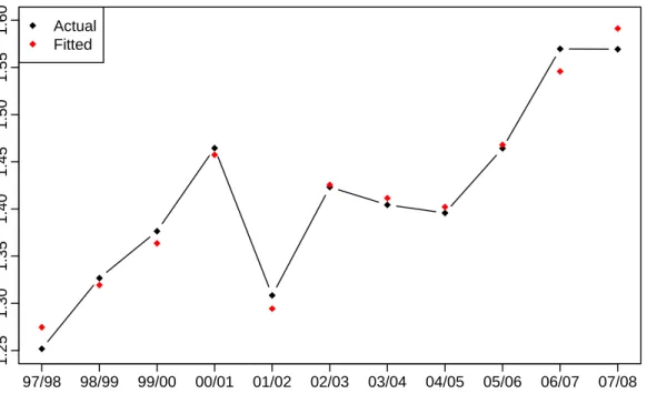
Year Annual demand 1.25 1.30 1.35 1.40 1.45 1.50 1.55 1.60 97/98 98/99 99/00 00/01 01/02 02/03 03/04 04/05 05/06 06/07 07/08 Actual Fitted
Figure 7: Actual summer demand and summer demand predicted from the model for annual
data.
4.3 Model fitting
We investigate the predictive capacity of the model by looking at the fitted values. Fig. 7
shows the fitted annual median demand. It can be seen that the variables have captured the underlying trend in electricity demand remarkably well.
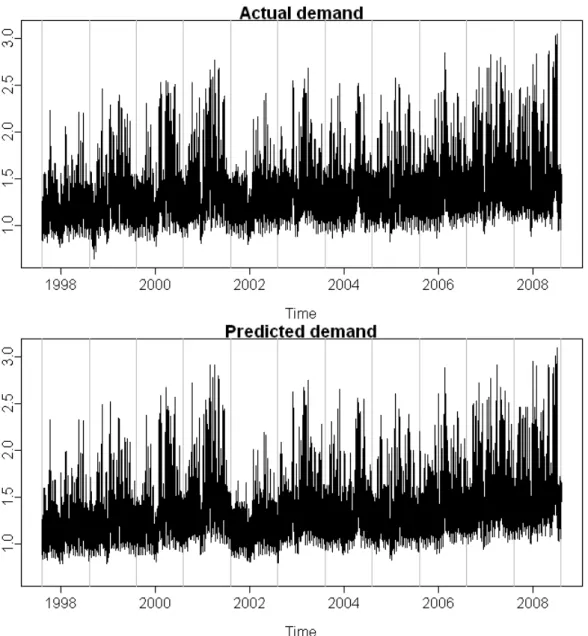
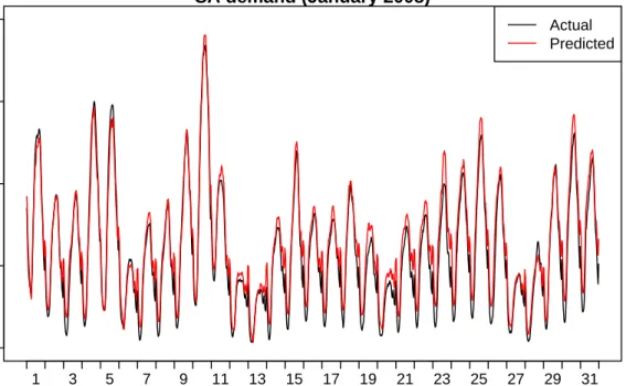
We combine these annual fits with the fits from the half-hourly model (5), to obtain estimated demand at each period of historical data. These are shown in Fig. 8. Fig. 9illustrates the model prediction for January 2008. The fitted and actual values are almost indistinguishable showing that the vast majority of the variation in the data has been accounted for through the driver variables.
These “predicted” values are not true forecasts as the demand values from these periods were used in constructing the statistical model. Consequently, they tend to be more accurate than what is possible using true forecasts.
The difference between actual demand and fitted demand are known as the residuals; these values are shown in Fig. 10. In this case, the MAE is 51.4 MW or about 2% of the total variation in demand.
Figure 8: Time plots of actual and predicted demand.
The out-of-sample forecast accuracy will, on average, be worse than the in-sample forecast accuracy. In other words, the MAE calculated on out-of-sample forecasts will be higher than the MAE calculated above on in-sample predictions. In Section 6.2we will consider out-of-sample forecast evaluation for the summer of 2007/08.
SA demand (January 2008) Date in January SA demand (GW) 1.0 1.5 2.0 2.5 3.0 1 3 5 7 9 11 13 15 17 19 21 23 25 27 29 31 Actual Predicted
Figure 9:Actual and predicted demand for the first three weeks of January 2008.
5 Temperature simulation
For forecasting, we will need future values of the input variables, i.e. temperatures and economic data. We obtained the long-term GSP forecasts and pricing scenarios from ESIPC. To simulate the temperatures, we propose a new double seasonal block bootstrap method that involves blocks of variable length and variable start position for producing the distribution of half-hourly temperatures across the year. The effectiveness of the proposed method has been validated by reproducing the probability distribution of historical demand using simulated temperatures.
5.1 Bootstrap temperature resampling
Single season block bootstrap
The method of bootstrapping involves randomly resampling historical data. With time series, it is important to preserve any seasonal or trend patterns as well as the inherent serial cor-relation. The standard method for bootstrapping time series is the “block bootstrap” (Politis,
2003) which involves taking random segments of the historical time series and pasting them together to form new artificial series. There are obviously a very large number of such series that could be formulated in this way. A key parameter in the technique is the length of each segment. This needs to be long enough to capture the essential serial correlations in the data, but short enough to allow a large number of possible simulated series to be generated. When applied to seasonal time series, it is important that the length of each segment or block is a multiple of the length of the seasonal period. Politis (2001) calls this a “seasonal block bootstrap” although we will call it a “single season block bootstrap” to distinguish it from the double seasonal version to follow.
In a single season block bootstrap, a bootstrap series consists of whole seasons from the his-torical data, pasted together in a different order from how they were observed. For example, if this was applied to quarterly data from 1980–2007, then the seasonal period is four quarters or one year. A bootstrapped series of the same length as the original series would consist of a shuffled version of the data, where the data for each year stays together but the years are rearranged. For example, it may look like this:
In this paper, we will apply this approach to residuals from a fitted model which have a sea-sonal period of 48 half-hourly periods or one day. The series also show some serial correlation up to about 14 days in length. So we could sample in blocks of 14 days, or 672 time periods. The whole series would be divided into these blocks of length 14 days. In ten years of data (each of length 151 days), we would have 107 complete blocks as follows:
Block 1 Block 2 Block 3 Block 4 . . . Block 107
where Block 1 consists of observations from days 1–14, Block 2 consists of observations from days 15–28, and so on.
Then a bootstrap sample is obtained by simply randomly resampling from the 107 blocks. For example, the bootstrap series may be constructed as follows:
Block 105 Block 73 Block 39 Block 54 . . . Block 5
Double season block bootstrap
The above approach is not suitable for temperature simulation because temperatures contain two types of seasonality: daily seasonality as well as annual seasonality. If we were to take the whole year as the seasonal period, there would be too few years to obtain enough variation in the bootstrap samples.
Consequently, a new approach is required. We extended the idea of Politis (2001) for time series such as half-hourly temperatures that involve two seasonal periods. Specifically, we divide each year of data into blocks of length 48mwheremis an integer. Thus, each block is of length mdays. For the sake of illustration, supposem=9 days. Then block 1 consists of the first 9 days of the year, block 2 consists of the next 9 days, and so on. There are a total of 151/9=16.8 blocks in each year. The last partial block will consist of only 7 days.
Then the bootstrap series consists of a sample of blocks 1 to 17 where each block may come from a different randomly selected year. For example, block 1 may come from 1999, block 2 from 1996, block 3 from 2003, and so on. The randomly selected years give rise to a large range of possible bootstrapped series.
B1:1997 B2:1997 B3:1997 B4:1997 . . . B17:1997 B1:1998 B2:1998 B3:1998 B4:1998 . . . B17:1998 B1:1999 B2:1999 B3:1999 B4:1999 . . . B17:1999 .. . B1:2007 B2:2007 B3:2007 B4:2007 . . . B17:2007
Then one possible bootstrap series may look like this.
B1:2007 B2:2005 B3:2002 B4:2001 . . . B17:1999 B1:1999 B2:2007 B3:2002 B4:1999 . . . B17:1998 B1:2002 B2:1997 B3:2003 B4:2001 . . . B17:2004 .. . B1:2003 B2:2003 B3:2004 B4:2006 . . . B17:1997
The difference between this and the previous single season block bootstrap is that here, the blocks stay at the same time of year as they were observed, although they may randomly move between years.
One problem with this double seasonal block bootstrap method is that the boundaries between blocks can introduce some unrealistic large jumps in temperature. However, this behaviour only ever occurs at midnight, thus, the phenomenon is unlikely to be a problem for our simu-lation purposes since we are interested in high temperature.
As explained above, the number of possible values the simulated series can take on any given day is limited to the specific historical values that have occurred on that day in previous years. With ten years of historical data, there are only ten possible values that any specific point in the simulated series can take. While calculating statistics such as probability levels for individual days, it becomes a problem as there is insufficient variation to obtain accurate estimates.
Consequently, we introduce some variation in length and position. That is, instead of having blocks of fixed lengthm, we allow the blocks to be of length betweenm−∆days andm+ ∆ days where 0 ≤∆ < m. Further, instead of requiring blocks to remain in exactly the same location within the year, we allow them to move up to ∆ days from their original position. This has little effect on the overall time series patterns provided ∆ is relatively small, and allows each temperature in the simulated series to take a greater number of different values. We use a uniform distribution on(m−∆,m+ ∆)to select block length, and an independent
uniform distribution on(−∆,∆)to select the variation on the starting position for each block. This “double seasonal block bootstrap with variable blocks” performs much better in produc-ing the distribution of temperatures on a given day due to the larger number of potential values the simulated temperatures can take.
The simulated temperatures are actually adjusted slightly by adding some additional noise to allow the distribution of daily maximum temperatures to closely match those observed since 1900. The same noise value is added to each time period in a block and to both temperature sites. This ensures the serial correlations and the cross-correlations are preserved.
5.2 Probability distribution reproduction
To validate the effectiveness of the proposed temperature simulation, we reproduce the prob-ability distribution of historical demand using known economic values but simulating temper-atures, and then compare with the real demand data.
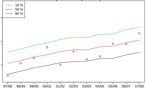
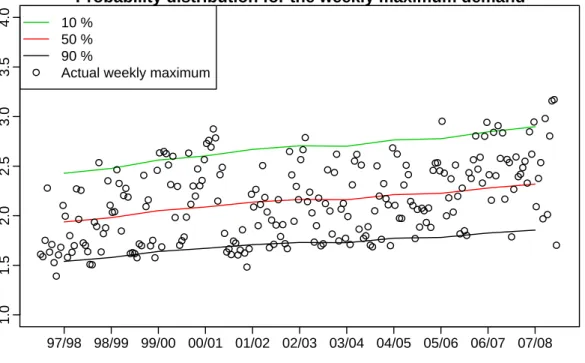
Figure11 shows PoE levels for all years of historical data using known economic values but simulating temperatures. These are based on the distribution of the annual maximum in each year. Figure12shows similar levels for the weekly maximum demand. There are three annual
PoE (annual interpretation)
Year PoE Demand 2.5 3.0 3.5 97/98 98/99 99/00 00/01 01/02 02/03 03/04 04/05 05/06 06/07 07/08 10 % 50 % 90 % ● ● ● ● ● ● ● ● ● ● ●
Figure 11: PoE levels for all years of historical data using known economic values but simulating
Probability distribution for the weekly maximum demand Year Demand 1.0 1.5 2.0 2.5 3.0 3.5 4.0 97/98 98/99 99/00 00/01 01/02 02/03 03/04 04/05 05/06 06/07 07/08 ● 10 % 50 % 90 %
Actual weekly maximum
●● ● ● ●● ● ● ●● ● ● ● ● ●● ● ● ● ●● ● ●● ●● ● ● ●● ● ● ●● ● ● ● ●●● ●●●● ●● ● ●● ●● ● ● ● ● ●● ● ● ● ● ● ●● ● ● ● ● ● ● ● ●● ● ●●● ● ● ● ●● ● ●●● ●● ●● ● ● ● ● ● ● ● ● ● ● ● ● ● ● ● ● ● ● ● ● ● ● ● ● ● ● ● ● ● ● ● ● ● ● ● ●● ● ● ● ● ● ● ● ●● ● ● ● ● ●● ● ● ●● ● ●● ● ● ● ● ● ● ● ● ● ● ● ●● ● ● ● ●● ● ● ● ●● ● ● ● ●●●● ● ● ● ● ● ● ● ● ● ● ● ● ● ● ● ● ● ● ● ● ● ● ● ● ● ● ● ● ● ●● ● ● ● ●●● ● ● ● ● ● ● ● ● ● ● ● ● ●● ●
Figure 12: Probability distribution of the weekly maximum demand for all years of historical
data using known economic values but simulating temperatures.
maximums above the 50% PoE level, two annual maximums below the 90% PoE level and no annual maximums above the 10% PoE levels. Of the 231 historical weekly maximum demand values in the past eleven summers, there have been nineteen above the 10% distribution level and twenty-one below the 90% distribution level. Therefore, it can be inferred that the reproduced probability distribution are within the ranges that would occur by chance with high probability (based on a binomial distribution). This provides good evidence that the forecast distributions will also be reliable for future years.
6 Forecasting and evaluation
We now forecast the distribution of annual and weekly peak electricity demand up to ten years ahead, and evaluate the model performance by comparing the forecasting results with the real demand data for summer 2007/2008.
6.1 Forecasting results
Forecasts of the distribution of demand are computed by simulation from the fitted model as described above. The temperatures at two locations are simulated from historical values
observed in 1997–2008 using the proposed double seasonal bootstrap with variable length. A total of 2000 years of temperature profiles were generated in this way for each year to be forecast.
Three different future scenarios for GSP, major industrial loads and average retail price were provided by ESIPC and are shown in Fig. 13. Future major industrial loads have been set based on the expected level of activity at these sites
The simulated temperatures, known calendar effects, assumed values of GSP, electricity price and major industrial demand, and simulated residuals, are all combined using the fitted sta-tistical model to give simulated electricity demand for every half-hourly period in the years to be forecast. Thus, we are predicting what could happen in the years 2008–2018 under these assumed economic and demographic forecasting scenarios, but allowing for random variation in temperature events and other conditions.
To simulate the major industrial demand,ot,p, we assume that it takes the formot,p=¯ot+ut,p
where ¯otis the annual major industrial demand andut,pis a (serially correlated) residual term that is independent of all other terms in the model. We use another single seasonal block bootstrap of length 20 days to simulateut,p and assume ¯ot is equal to the specified values in Fig.13(the low and base values are identical).
Probability distributions
We calculate the forecast distributions of the weekly maximum half-hourly demand for any randomly chosen week in summer, and the annual maximum half-hourly demand, using ker-nel density estimation (Silverman, 1986). Fig. 14 shows the simulated annual maximum demand densities for 2008/2009 – 2018/2019. Similarly, Figure 15 shows the simulated weekly maximum demand densities for 2008/2009 – 2018/2019.
South Australia GSP
Year
billion dollars (05/06 dollars)
2000 2005 2010 2015 50 60 70 80 90 100 High Base Low
Average electricity prices
Year c/kWh 2000 2005 2010 2015 12 13 14 15 16 17 High Base Low
Major industrial offset demand
Year MW 2000 2005 2010 2015 0 200 400 600 800 High Base Low
Figure 13: Three future scenarios for major industrial demand and South Australia’s GSP and
average electricity price. The bottom panel shows the predicted effect on annual median demand for South Australia.
3 4 5 6 0.0 0.5 1.0 1.5 Low Demand (GW) Density 3 4 5 6 0.0 0.5 1.0 1.5 Base Demand (GW) Density 3 4 5 6 0.0 0.5 1.0 1.5 High Demand (GW) Density 2008/20092009/2010 2010/2011 2011/2012 2012/2013 2013/2014 2014/2015 2015/2016 2016/2017 2017/2018 2018/2019
2 3 4 5 0.0 0.2 0.4 0.6 0.8 Low Demand (GW) Density 2 3 4 5 0.0 0.2 0.4 0.6 0.8 Base Demand (GW) Density 2 3 4 5 0.0 0.2 0.4 0.6 0.8 High Demand (GW) Density 2008/20092009/2010 2010/2011 2011/2012 2012/2013 2013/2014 2014/2015 2015/2016 2016/2017 2017/2018 2018/2019
Probability of exceedance
We also calculated “probability of exceedance” levels from the simulated data. Suppose we are interested in the level x such that the probability of the annual maximum demand exceeding x isp. Then x is the(1−p)th quantile of the distribution of the simulated demand values, which we compute using the approach recommended byHyndman and Fan(1996).
PoE values based on the annual maxima are plotted in Fig.16, along with the historical PoE values and the observed annual maximum demand values. Fig.17shows similar levels for the weekly maximum demand wherepis the probability of exceedance in a single year.
Annual POE levels
Year PoE Demand 2 3 4 5 6 97/98 99/00 01/02 03/04 05/06 07/08 09/10 11/12 13/14 15/16 17/18 ● ● ● ● ● ● ● ● ● ● ● ● 1 % POE 5 % POE 10 % POE 50 % POE 90 % POE
Actual annual maximum
Figure 16: Probability of exceedance values for past and future years. High scenario: dotted
Probability distribution for the weekly maximum demand Year Demand 1 2 3 4 97/98 99/00 01/02 03/04 05/06 07/08 09/10 11/12 13/14 15/16 17/18 ●● ● ● ●● ● ● ●● ● ● ● ● ●● ● ● ● ●● ● ●● ●● ● ● ●● ● ● ●● ● ● ● ●●● ●●●●●● ● ●● ●● ● ● ● ● ●● ● ● ● ● ● ●●● ● ● ● ● ● ● ●● ● ●● ● ● ● ● ●● ● ●●● ●● ●● ● ● ● ● ● ● ● ● ● ● ● ● ● ● ● ● ● ● ● ●● ● ● ● ● ● ●● ● ●● ● ● ● ● ●● ● ● ● ● ● ● ● ●● ● ● ● ● ●● ● ● ●●● ●● ● ● ● ● ● ●● ● ● ● ● ●● ● ● ● ●● ● ● ● ●● ● ● ● ●●●● ● ● ● ● ● ● ● ● ● ● ●● ● ● ● ● ● ● ● ● ● ● ● ● ● ● ● ● ● ●● ● ● ● ●●● ● ● ● ● ● ● ● ● ● ● ● ● ●● ● ● 10 % POE 50 % POE 90 % POE
Actual weekly maximum
Figure 17: Probability distribution levels for past and future years. High scenario: dotted lines.
Base scenario: solid lines. Low scenario: dashed lines.
6.2 Model evaluation
To evaluate the forecasting performance, we compare the actual demand of the last summer of data (2007/2008) with two different types of predictions: ex ante forecasts and ex post forecasts. Specifically,ex ante forecastsare those that are made using only the information that is available in advance; consequently, we calculate 2007/08 summer demand using eco-nomic conditions as assumed in 2007 and simulated temperatures based on models for data up to 2007.
On the other hand,ex post forecastsare those that are made using known information on the “driver variables”. In this evaluation, ex post forecasts for 2007/08 summer are calcu-lated using known economic conditions in 2007 and known temperatures for the summer of 2007/08. We do not use data from the forecast period for the model estimation or variable selection. Ex post forecasts can assume knowledge of the input or driver variables, but should not assume knowledge of the data that are to be forecast.
The difference between the ex ante forecasts and ex post forecasts will provide a measure of the effectiveness of the model for forecasting (taking out the effect of the forecast errors in the input variables).
Figure18illustrates the ex ante forecast density function for maximum weekly demand and maximum annual demand for 2007/08.
These graphs demonstrate that the actual demand values fit the ex ante forecast distribu-tions remarkably well. The upper graph provides the best evidence of the performance of the model. In this case, the 21 actual weekly maximum demand values all fall within the region predicted from the ex ante forecast distribution. Although there is only one annual maxi-mum demand observed, the bottom graph shows that this also falls well within the predicted region. Figure18also indicates the effect of updating and including the ex post economic in-formation subject to the use of simulated temperatures and random components. The graphs also show that the uncertainty associated with the economic variables is very small compared to the uncertainty due to temperatures and other sources of variation. However, there is con-siderable uncertainty associated with the economic forecasts themselves, especially over the longer term, since economic relationships might change over time (e.g., uncertainties about the impact of carbon pricing, adoption of new efficiency measures and new technologies).
7 Conclusion
In this paper, we have proposed a new semi-parametric methodology to forecast the density of long-term annual and weekly peak electricity demand. The key features of our model are that it provides a full density forecast for the peak demand several years ahead, with quantifiable probabilistic uncertainty. It captures the complex non-linear effect of temperature and allows for calendar effects, price changes, economic growth, and other possible drivers. The forecasting results demonstrate that the model performs remarkably well on the historical data.
As with any new methodology, there are some areas for possible future improvement. For in-stance, we assume that the long-term temperature patterns are stable in this work; however, climate change is likely to have much more complex and subtle effects on future tempera-ture patterns and distributions. We are endeavouring to incorporate some long-term climate change predictions into our model. Another area for development is to increase the number of temperature sites in the model. For South Australia’s geographically concentrated population, two temperature sites may be adequate. But for other regions, a larger number of temperature sites would be desirable.
1.0 1.5 2.0 2.5 3.0 3.5 4.0 0.0 0.2 0.4 0.6 0.8 1.0
Density of weekly maximum demand
Demand (GW)
Density
Ex ante Ex post
Actual weekly maximum
1.0 1.5 2.0 2.5 3.0 3.5 4.0
0.0
0.5
1.0
1.5
Density of annual maximum demand
Demand (GW)
Density
Ex ante Ex post
Actual annual maximum
Figure 18: Ex ante probability density functions for half-hourly, weekly maximum demand and
Acknowledgment
The authors would like to thank the South Australian Electricity Supply Industry Planning Council (ESIPC) for supplying the data used in this paper. We also would like to thank Gary Richards and David Swift of ESIPC for their valuable comments and feedbacks on this research work.
References
Al-Hamadi, H. M. and S. A. Soliman (2005) Long-term/mid-term electric load forecasting based on short-term correlation and annual growth, Electric Power Systems Research, 74, 353–361.
Amjady, N. (2006) Day-ahead price forecasting of electricity markets by a new fuzzy neural network,IEEE Trans. Power Syst.,21(2), 887–896.
Amjady, N. (2007) Short-term bus load forecasting of power systems by a new hybrid method, IEEE Trans. Power Syst.,22(1), 333 –341.
Box, G. E. P. and D. R. Cox (1964) An analysis of transformations,Journal of the Royal Statis-tical Society, Series B,26(2), 211–252.
Chen, B. J., M. W. Chang and C.-J. Lin (2004) Load forecasting using support vector machines: a study on EUNITE competition 2001,IEEE Trans. Power Syst.,19(4), 1821˝U1830.
Fan, S. and L. Chen (2006) Short-term load forecasting based on an adaptive hybrid method, IEEE Trans. Power Syst.,21(1), 392–401.
Harrell, Jr, F. E. (2001) Regression modelling strategies: with applications to linear models, logistic regression, and survival analysis, Springer, New York.
Hastie, T. and R. Tibshirani (1990)Generalized additive models, Chapman & Hall/CRC, Lon-don.
Hippert, H., C. Pedreira and R. Souza (2001) Neural networks for short-term load forecasting: A review and evaluation,IEEE Trans. Power Syst.,16(1), 44 – 55.
Huang, S. J. and K. R. Shih (2003) Short-term load forecasting via ARMA model identification including nonGaussian process considerations,IEEE Trans. Power Syst.,18(2), 673–679. Hyndman, R. J. and Y. Fan (1996) Sample quantiles in statistical packages, The American
Kandil, M. S., S. M. El-Debeiky and N. E. Hasanien (2002) Long-term load forecasting for fast developing utility using a knowledge-based expert system,IEEE Trans. Power Syst., 17(2), 491 – 496.
Kermanshahi, B. (1998) Recurrent neural network for forecasting next 10 years loads of nine Japanese utilities,Neurocomputing,23, 125–133.
McSharry, P. E., S. Bouwman and G. Bloemhof (2005a) Probabilistic forecast of the magnitude and timing of peak electricity demand,IEEE Trans. Power Syst.,20(2), 1166–1172.
McSharry, P. E., S. Bouwman and G. Bloemhof (2005b) Probabilistic forecasts of the magnitude and timing of peak electricity demand,IEEE Transactions on Power Systems,20, 1166–1172. Morita, H., T. Kase, Y. Tamura and S. Iwamoto (1996) Interval prediction of annual maxi-mum demand using grey dynamic model,International Journal of Electrical Power & Energy Systems,18(7), 409–413.
Politis, D. N. (2001) Resampling time series with seasonal components, inFrontiers in data mining and bioinformatics: Proceedings of the 33rd symposium on the interface of computing science and statistics, pp. 619–621.
Politis, D. N. (2003) The impact of bootstrap mathods on time series analysis,Statistical Sci-ence,18(2), 219–230.
Power Systems Planning and Development (2005) Load forecasting white paper, Tech. rep., National Electricity Market Management Company Limited.
Ramanathan, R., R. F. Engle, C. W. J. Granger, F. Vahid-Araghi and C. Brace (1997) Short-run forecasts of electricity loads and peaks,International Journal of Forecasting,13, 161–174. Ruppert, D., M. P. Wand and R. J. Carroll (2003)Semiparametric regression, Cambridge
Uni-versity Press, New York.
Silverman, B. W. (1986)Density estimation for statistics and data analysis, Chapman and Hall, London.
Song, K. B., Y. S. Baek, D. H. Hong and G. Jang (2005) Short-term load forecasting for the holidays using fuzzy linear regression method,IEEE Trans. Power Syst.,20(1), 96–101. Taylor, J. W. (2003) Short-term load electricity demand forecasting using double seasonal
exponential smoothing,Journal of the Operational Research Society,54, 799–805.
Weron, R. (2006)Modeling and forecasting electricity loads and prices: A statistical approach, Wiley Finance.