Leaf Recognition with Deep Learning and Keras using GPU computing

Leaf Recognition with Deep Learning and

Keras using GPU computing

Jes ´us L ´opez Barrientos

18/02/2018

Abstract–Our work is about using Deep Learning for leaf recognition using Keras and GPU compu-tation. We used 17 CNNs of”Kaggle” [1], a Machine Learning training webpage that using simple challenges with prizes help people to learn how to use Deep Learning. Kaggle made a challenge in August, 30th, 2016 that was about Leaf Recognition. In that challenge more than 1500 users participated in it. They made teams to participate and we grab 17 codes of them to see how their codes was working. We updated the codes, because they were written in 1.0 version of Keras, and we use 2.0.6 version and then we made a ranking to test their accuracy in leaf recognition using the dataset provided by kaggle. Also we downloaded two more datasets to make more tests with them. On the other hand, we found two papers in ”the ImageClef Competition” [2], and we implemented them from the beggining to see how simple is to transform a paper into code. ECOCUAN team, from 2015, used a tunned AlexNet CNN and KDETUT, from 2017, used a ResNet50 modified CNN. Another paper found on the net was one that use ResNet26 CNN, so we think that was a good idea to make a ranking of the three of them to see which is better.

Key Words– Deep Learning, Keras, CNN, Convolutional Neural Network, Tensorflow, Leaf Recognition, ResNet, AlexNet, LeNet, Kaggle, ImageClef

F

1

INTRODUCTION

H

OW make to learn a computer machine the specie of a tree leaf? That is the question of my work. Human eye see a leaf, but, what is the thing that makes us to recognize the specie of that leaf? we can see the shape of the leaf, but there are so much similar leaf of some species that are the same. So we can see the shape and the color of the leaf, but there are also some other features that can be learned to classify that leaf.

A Convolutional Neural Network makes that learning au-tomatical making segmentation of the leaf image. The al-gorithm segments the image and extract the best features for each segment for lately join the image and make a pre-diction of the class. That algorithm of automated learning is needed because of the big number of classes that exists in the world, and the impossibility to make people do a database containing all the features of all the leaf types. So that Network will do all the work for itself.

•Author: Jes´us L´opez Barrientos

•Contact E-mail: [email protected]

•Branch: Computing

•Tutor: Fernando Vilari˜no Freire (Computer Science Department)

•Contact E-mail: [email protected]

•2017/18 Course

That paper is divided in nine sections where we will ex-plain state-of-the-art of Deep Learning through the time, how all the codes are implemented, wich Convolutional Neural Network is in the code and what is our method for comparing the codes to make the ranking.

Also we will show you how we managed to make my ranking of all the Kaggle codes using two datasets, Kaggle dataset containing 990 binary leaf images of 99 classes of leaves and Middle European Woods 2012 [3] dataset, con-taining 9745 binary leaf images of 153 classes of leaves.

And our investigation of the three papers that we imple-mented, using two datasets, Flavia [4] dataset containing 1907 fully color images of 32 classes of leaves.

2

A

LITTLE

CNN’S HISTORY

D

EEPLEARNING was very hard to use before 90’s because the requirements for implement a good neural network was not enough with the comput-ers of that epoch. So in 1998, when the computcomput-ers could do powerful calculations, Yann LeCunn et al. [5] create a neural network to make an OCR, a postal code digit recog-nition. They used de MNIST dataset to train their network and they archieved a 99,7% of accuracy in their predictions. Their Net was based on one Convolutional layer followed by one Max pool layer.

In 2012, Alex Krizhevsky et al. participated in ImageNet Large Scale Visual Recognition Challenge [6] and proposed a new Convolutional Network named AlexNet [7] that out-performed the second best model. They archieved a 16% classification error and the second best was 26%. They modified the LeNet estructure to make it deeper with par-alelization of layers in two lines.

In 2013, Matthew Zeiler and Rob Fergus presented a new Convolutional Network named ZFNet [8] that was an im-provement of AlexNet modifying some parameters of the net. They win the ImageNet 2013 contest. They archieved a 11% classification error.

In 2014, Szegedy et al. from Google presented a new Network named GoogLeNet [9] that implements an Incep-tion Modulethat reduces the parameters of the net and uses an Average Pooling instead of Fully Connected layers in the top of the net. With that network they win the contest with a 6% classification error.

The second place of the 2014 competition was VGGNet [10], they archieved a 7% of classification error and they based their implementation on making their Network much deeper. They make a 16-layer Network to demostrate that more deep the net more best performance archieved.

In 2015, Kaiming He et al. won the contest archieving a 3% classification error with their new Network named ResNet [11]. They use convolutional blocks that imple-ments some convolutional layers followed by some batch-normalizations. In the first convolutional block of each fase they let the net to choose if is best to apply all the block to the data or skip the entire block and use only one con-volution of the inputs. Also they don’t apply some fully-connected layers in top of the net.

3

S

TATE

-

OF

-

THE

-

ART

Y

EAR 2017 was the last that the PlantClef compe-tition was done. The result of the competition shows that the best execution of a CNN scored a 96’2% accuracy with a dataset containing Trusted images and Noisy web data about plants. The CNN of the winner was built with 3 types of CNN, GoogLeNet, ResNet-152 and ResNetXT and the prediction was the average of the three of them. But the second best team, scored a 92,7% accuracy only making a prediction with a modified ResNet-50 CNN.

So Teams actually works in a merged CNN using differ-ent types of CNN.

Also, nowadays exists so many apps that uses CNN to make plant recognition. The most important is the Plant-Net [13] app. They use a modified GoogLePlant-Net CNN pre-trained with ImageNet dataset and periodicaly pre-trained with their own PlantNet dataset, a dataset that all people can con-tribute with their pictures. They use that CNN because they made the app in 2015, so the best CNN in that year was GoogLeNet. If you want to know more about that app you can see a review made by them namedPl@ntnet app in the era of deep learning[14].

Even Apple are using deep learning in their products[12], as face-recognition or SIRI speak recognition, so today is even easier to build an app with deep learning implementa-tion.

4

METHODOLOGY

T

HEmethodology of our work is to run ten codes ob-tained from Kaggle with CNNs with kaggle (that has images and numerical shapes of leaves) and MEW2012 datasets and to compare the results obtained, also, we converted the Flavia color dataset into Flavia thresholded to run with them. We also updated the codes because they were made with 1.0 version of Keras. We have 2.0.6 version, but, fortunately, the only differences between them was the order of some arguments of the Conv2d layer and the parameters to feed fit function. The problem arrives with 2.0.8 version of keras, that made our code not to run at all, so we decided not to upgrade and continue with 2.0.6. We also have 7 codes with only fully-connected layers, that only works with numerical shapes of leaves, to compare it with using images or images+shapes. For the three papers obtained, we implemented the CNNs only reading the pa-pers and understanding their explanations that althoug they contais explanation images, sometimes is hard to under-stand. We ran the three papers with Flavia dataset because it is in color and simple enought to run fast and obtain good results. In that ranking we made a cross-validation procces with Sklearn cross val score function to obtain the accuracy number. We implemented it with Python using Keras (with Tensorflow backend) and Sklearn. We recommend to use Anaconda[15] because it installs all what you want only by typing the install method found in their website to install the packages you want, and it works on all systems, windows, linux and Mac OS.

Also it has Spyder editor, a powerful python editor that has all the functionalities needed to write and run the codes, and also view the results in the ipython console.

It also has the option to create a enviroment to install the packages and let the system untouched. It is essential if you have another version of python installed and you don’t want to have incompatibilities with it.

4.1

Keras Python Library

Keras[16] is a python library built by Franc¸ois Chollet

that helps to build convolutional neural networks by using very easy to use functions that are being updated constantly thanks to the improvements proposed by github users. That library helps a lot to build it because makes transparent to the user the usage of tensorflow backend, that has too much instructions to build the network. To build your network it is as simple as create a combined model function that cre-ates all the layers you want, only needing one function per layer. You only have to add the arguments to the functions, the number of neurons, filter size and stride number and it is all. Keras let you use the CPU or GPU versions of it. If you have Nvidia graphic card that is CUDA capable, you can run GPU version. It makes the network to learn faster than the CPU version. The difference is like 30 seconds to learn 1 epoch with CPU version and 5 seconds in a GPU version. It is very important in dataset containing GB of images because the difference is between 1 day or 1 week of learning. For example in ImageNet[17] dataset that con-tains 150.000 images of 1000 classes. Another advantage of Keras is that Google is behind it working to improve that library so the improvements appears quickly. The

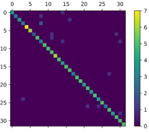
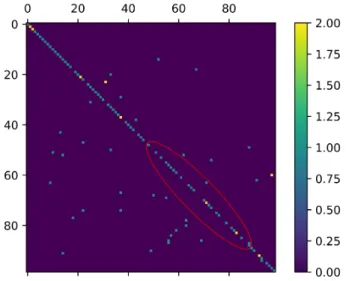
disad-Fig. 1: Confusion Matrix

vantage of Keras is that newer versions are not backwards compatible, so you has to rewrite all the code to run with it. Keras has two learning methods, the normalfit()function that only specifying the training dataset and if you want an-other validation dataset, and the number of epochs to train it will train our network for the number of epochs. You can also specify another argument,batchthat works to feed the network in groups of images that you specify in the batch number. It is useful to train the network faster. The other function is the fit generator() function. That function is very helpful to train our network with too big datasets, for example the ImageNet dataset as you can feed the network reading batches of images at a time specifying a generator function that reads the images and gives it to the CNN. In fit function you has to put all the dataset to it, imagine to load 60GB of images... The problem with Keras fit function is that it returns not the best model of the training, it returns the last model trained by it so you have to add a callback argument that stores the best model trained in a file you can specify.

4.2

Sklearn Python Library

Sklearn[18] is a library for python that let us use some functions very useful to test the integrity of our CNN. That functions are the ones to create a matrix function, make a classification report and a cross-validation function. We modified the cross-validation function because it uses fit function without callbacks so it doesn’t show the best result for the training so we added that to make the result more accurated.

As you can see in Fig.1, the confusion matrix show you the number of positive results in the diagonal of the image and the other around are the negative results. For example, you can see one 3 class classified as a 8 class.

4.3

Datasets

The datasets used in our work are: Kaggle dataset, used by the kaggle contestants provided by the kaggle webpage, theMiddle and European Woods 2012 dataset, a dataset found on internet that contains the same types of images that kaggle dataset has but with a lot of more images per class, so it is useful to compare the CNNs with a large dataset. And the last one is theFlavia dataset. That dataset is used by the last paper found, the one that uses the ResNet26 CNN.

It is in color so it is used to train our three papers implemen-tations and make the comparisons. For more tests, we trans-formed the Flavia dataset into a thresholded Flavia dataset, we named it Flaviabw. We used it to train the kaggle codes.

4.3.1 Kaggle dataset

The Kaggle dataset contains 990 images of 99 classes of leaves. All the images are thresholded, so they are black and white images. Also contains a .csv document contain-ing shape, texture and margin numerical features of all the leaves. That dataset is the one provided by kaggle in their competition. The original dataset has more images, but they use a part of it as a test data, so they don’t provide the tags for them so we can not use that as a train or test so we dis-card them.

(a) Kaggle leaf (b) MEW 2012 leaf

Fig. 2

4.3.2 MEW2012

The Middle and European Woods 2012 contains 9745 im-ages of 153 classes of leaves. They are the same type as Kaggle, thresholded black and white images. It is the best way to test the CNNs without the numerical features be-cause it has more images of the same type.

4.3.3 Flavia

Fig. 3: Flavia leaf

The flavia dataset contains 1907 images of 32 classes. They are full color images but with a white background (Fig.3) so it only appears the leaf. It is used in the ResNet26 paper to train their CNN. We make a flavia thresholded dataset to test it with Kaggle CNNs because we think we can make the best comparison having more datasets to train with.

4.4

Convolutional Neural Networks

In this section we will explain a bit of what the networks we have to run are made up of. We will explain the layers

that have them and their neuronal structure. For the Kaggle codes, because they are so many, you can find their specifi-cation in the Annex.

4.4.1 CNNs from Kaggle competition

This website held a competition for classification of leaves using Machine Learning from August 30, 2016 to March 1, 2017. It involved more than 1500 groups that were try-ing to get a good classification in their leaderboard but the three winners were taken without taking into account the result. So the winners of the contest were not going to be the ones that got a better classification but three groups that their codes were the most excellent. A code may not give a better classification than the first but it may be much bet-ter structured or with betbet-ter results with a larger dataset, so the judges checked the code personaly to get the best three of them. One of them was Albhijeet Mulgund who made a neural network based on LeNet architecture with Keras (it is one of the codes that we have for our work). It was a role model for many other participants of the contest.

Fig. 4: LeNet Architecture

These networks are based on the network called LeNet (Fig. 4), which is composed of one or two convolutional layers followed by a normalization layer and a pooling layer. Only one contestant used the AlexNet network, but having hardware limitations on his computer, since he used the CPU for calculations, he finally had to opt for a simple LeNet. Although in our work we have executed the two net-works to see their results. Some of these netnet-works use the numerical shapes provided in the kaggle dataset, they are introduced just after the convolutional layers, giving the pa-rameters directly to the Fully-Connected (Dense) layers. To check if the results are correct, we have also obtained seven networks that only use Dense layers, using only the shapes of the image to see if the results with or without images are best, worst or equal.

4.4.2 CNN from ImageClef Competition

Then we tried to transform into a CNN some papers found in ImageClef competition to see the ease of make CNN with keras. Keras is a powerful and simply to use python library, and it only takes a few hours to make a CNN work, and it is without knowing something about keras. When you get used to it, it only takes a few minutes to create one. The competitors of the contests uses the dataset pro-vided by ImageClef, but that dataset was GB long and it not only has simple images of leaves, it also contains images of branches, flowers and all the plant/tree with forest back-ground, so we decided not to use it because we don’t have all the time and equipment to test it well. In the other hand, Flavia dataset used in the ResNet26 paper was in color and small enought to use it with our implementations.

Fig. 5: Ecocuan Architecture

ECOCUAN Team ECOCUAN team[19] created a CNN using ZFNet model (tunned AlexNet) (Fig. 5). They re-duce the image size to 224x224, as they don’t say some-thing about normalizing we normalized it and yield it to the network. The network is made of five convolutional layers, and three MaxPooling layers after 1,2 and 5 convolution layers. They end the network with two fully-connected lay-ers with 4096 neurons and the last softmax fully-connected layer with the number of classes of the input for classifica-tion.

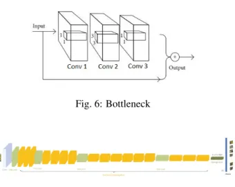
KDETUT KDETUT team[20] implements a modified ResNet50 architecture. ResNet architecture is based on ”bottleneck” building blocks (Fig.6). Each block has three convolutional layers and the possibility of skip all of them if the network thinks that is better not to apply them.

Fig. 6: Bottleneck

Fig. 7: ResNet50 Architecture

KDETUT team implemented two CNNs based on ResNet50 model. They modified it in two ways adding MaxPooling layer before (ResNetMP)(Fig.7) or after (ResNetMPD) the ResNet blocks. Also, they reduced the stride size of the convolutional layers from 2 to 1. They also resize the images to 224x224, rotated +-45o and hori-zontally flipped.

4.4.3 Resnet26

The group that makes that paper implemented a ResNet model with 26 layers[21] (Fig.8). That is interesting to test the better or worst results compared with ResNet50MP of KDETUT. It has 1 convolutional layer plus 8 ”bottle-neck” building blocks (3 convolutional layer) plus 1 fully-connected layer, so it has 26 layers.

They resize images to 224x224 pixels and then normal-ized.

Fig. 8: ResNet26 Architecture

5

EXPERIMENTAL

SETUP

For the networks obtained from Kaggle, we had to update the version of the Keras functions of them, since they used version 1.0 of Keras. Luckily, only the name of some func-tions and the order of the parameters of the calls changes, for the rest there was no need to modify something else. To facilitate the use of the networks, a template was made in which only the neural network had to be changed and enable or not the modification of the images, depending on whether the original network made modifications to them, such as, for example, rotate the images or reduce their size. The datasets of Kaggle, MEW2012 and Flaviabw were used, running each network for 200 epochs initially and increas-ing that value if necessary. For the networks of papers, we use the same template mentioned above, changing the net-work for the paper one and enabling the modifications that the paper use. These papers were not implemented with keras, for example the paper of the KDETUT team was im-plemented with Caffe, another library similar to keras, so we had to adapt it to Keras. Normally, the same modifica-tions are always made to the dataset, for example, adding the same image rotated, cropped and centered to build a new dataset, or changing the size of the images taking into account the type of image, for example, in the case of the dataset of kaggle, the images only have information about the margins, so we can reduce the image to 96x96 pixels without losing definition on it. On the other hand, in the Flavia dataset, being in color, it contains much more in-formation about each leaf and if we reduce the image too much we can lose information about it, for example, the texture of the leaf with reduced image will be lost. Doing the implementations of the networks of the papers we re-alized that it was not easy to find out what each network was alike so you have to understand the images, if any, very well, and if there are no images of the network, we have to read the description very well so as not to make a mistake in the sizes of the filters, or where the MaxPooling layers are placed. Although we can always send an email to the paper contact mail to ask about its implementation. In the case of the KDETUT team, we sent an email and they an-swered us with their network structure that although it was implemented with Caffe, we could adapt it to Keras without problems.

To train our model, we set the images to 0.8 train and 0.2 test, then we divided that train set in 0.8 train and 0.2 validation. With this we obtain the necessary train and val-idation datasets to train our network checking that it learns well without producing overfitting and then we run the test to see how well the CNN has learned. At each execution of the networks we obtained information about the accu-racy and loss of the model we train, and also showed some

graphs of them. We kept the graphs together with an im-age of the confusion matrix and a table that contained the classification report of the model.

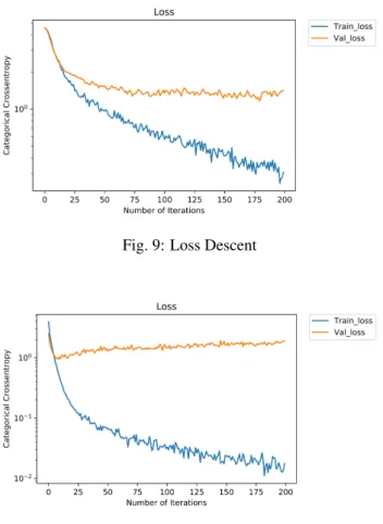
Fig. 9: Loss Descent

Fig. 10: Loss Increase

Checking the graphs obtained from each execution, we could know if it was necessary to increase the epochs or not so that the network would continue learning. If we look at the graph of Fig.9 we can see that the val loss line continues to fall, so it is necessary to increase the epochs since that val loss can continue to descend. In this case, we increased the epochs to 500 and in the epoch 360 we obtained the best model but the graph continued to decrease so we increased it to 1000 epochs and we obtained the best model in the 720, however, in Fig.10 we can see that the val loss line begins to rise in epoch 11 so the best training model for our network is in that epoch so although we can not ensure that doesn’t improve with more epochs at 100%, seeing the graph we can discard the option. We say that we can not assure it because for example with the network ResNet50 we obtain an increase of the val loss line at the beginning, and in the epoch 20 it begins to descend, and in a case of one Kaggle network, it not begins to classify well until epoch 500.

In the case of paper networks, we also did a 10-fold cross-validation to obtain an average value of our network accu-racy since by training the network with only some train and other test images we may have discarded the best images to train placing them as a test. For this we do a 10-fold cross-validation that divides our train into 10 sets and runs our training once for each set as a test and the rest for train, thus, at the end, we can obtain a mean value of the accuracy of our network.

To know the accuracy of our network, we use a sklearn library function that allows us to make a classification

report of our data. As we can see in Fig.11, we have 3 results, precision, recall and F1-score. Precision is the result of dividing the positive results of the current class by the total of the positive results that class has received.

Recallis the result of dividing the positive results of the current class by the total positive results that that class should have received. AndF1-scoreis the result of double Precision multiplied by Recall divided by the sum of Precision and Recall. For example, if we have a class A that has 6 test images, and receives 7 classifications of which 4 are correct (that is, 4 of those 6 images have been classified correctly), then we will have that:

precision= 4₇ = 0.57 recall=4₆ = 0.67 F1-score=0.57

0.67 = 0.85

With this we make an average of all the values to ob-tain the total of each results. We use the value of the F1-score as the accuracy of our network.

Fig. 11: Classification Report

6

RESULTS

T

HE results obtained from the runnings of the net-works were very ilustrating. For an easy under-standing they have been placed in classification ta-bles, which have been ordered by the best results and then by the number of epochs, from less to more. We also put the number of layers of each neural network since it is im-portant to draw conclusions. In this paper we only show the Accuracy tables since they are the ones that really interest us to knowing if our network classifies well or not.

6.1

Results from Kaggle CNNs

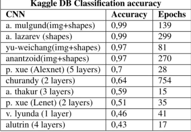
In the table 1 we can find the results of the runnings of the Kaggle networks with numerical shapes and images. For one network in particular was necessary to run it for more epochs since the learning graph continued decreasing until epoch 706.

TABLE 1: KAGGLERANKING

Kaggle DB Classification accuracy

CNN Accuracy Epochs

a. mulgund(img+shapes) 0,99 139 a. lazarev (shapes) 0,99 299 yu-weichang(img+shapes) 0,97 81 anantzoid(img+shapes) 0,97 270 p. xue (Alexnet) (5 layers) 0,7 28 churandy (2 layers) 0,64 754 a. thakur (3 layers) 0,59 15 p. xue (Lenet) (2 layers) 0,51 35 v. lyunda (1 layer) 0,46 41 alutrin (4 layers) 0,43 17

TABLE 2: KAGGLEONLYFEATURESRANKING

Kaggle DB only features Classification accuracy

CNN Accuracy Epochs Picubeisnot30 1 861 Guravjoshi 0,99 991 Ibprofin 0,99 995 Konstantin Tumalevich 0,98 724 Churandy 0,97 949 Michael Semeniuk 0,97 996 Prateek 0,97 999

In table 2 are the Neural Networks that only use the nu-merical features to learn. So they don’t use images as input, only numerical values. We trained them for 1000 epochs because all of them had down curves, but the results are mostly the best that can be. As its shown in the table, the re-sults of the numerical features only is better than the rere-sults of the images only. That is because that numbers are hand-writted and represents each leaf whith unique features. But in the real life, it is impossible to have all that numbers for all the leaf types, that is the reason that the CNN appeared, a system that can learn automaticaly without helping it.

TABLE 3: MEW2012 RANKING

MEW2012 Classification accuracy

CNN Accuracy Epochs

p. xue (Alexnet) (5 layers) 0,81 13 churandy (2 layers) 0,76 161 a. thakur (3 layers) 0,75 8 p. xue (Lenet) (2 layers) 0,75 23 anantzoid (4+4 layers) 0,75 232 a. mulgund (2 layers) 0,67 21 v. lyunda (1 layer) 0,61 18 yu-weichang (1 layer) 0,58 8 alutrin (4 layers) 0,57 9

In Table 3 you can see the ranking using MEW2012 dataset. In that ranking We put the number of layers that contains all the CNNs because it is important to see the

clas-sification with that parameter.

TABLE 4: FLAVIABW RANKING

Flaviabw Classification accuracy

CNN Accuracy Epochs

churandy (2 layers) 0,89 194 p. xue (Alexnet) (5 layers) 0,84 39 a. thakur (3 layers) 0,82 9 p. xue (Lenet) (2 layers) 0,79 32 a. mulgund (2 layers) 0,77 39 v. lyunda (1 layer) 0,73 14 yu-weichang (1 layer) 0,71 28 alutrin (4 layers) 0,7 32 anantzoid (4+4 layers) 0,56 245

In Table 4 it is shown the ranking using Flavia thresh-olded dataset. The number of classes in flavia threshthresh-olded are 32, so the networks had more images per class to train with.

TABLE 5: FLAVIA

Flavia Classification accuracy

CNN Accuracy Epochs

a. thakur (3 layers) 0,92 36 p. xue (Alexnet) (5 layers) 0,91 84 churandy (2 layers) 0,9 183 a. mulgund (2 layers) 0,87 70 p. xue (Lenet) (2 layers) 0,86 66 yu-weichang (1 layer) 0,82 54 v. lyunda (1 layer) 0,8 62 alutrin (4 layers) 0,78 62 anantzoid (4+4 layers) 0,46 112

In table 6 are shown the results of executing the Kaggle neural networks using Flavia color dataset. We only change the input layer of each network to accept 3 layer images as input. The results are only relevant to see how works their network structure with color dataset, as they are different networks from the original ones, because changing input dimension changes internally each layer of the network.

6.2

ECOCUAN, KDETUT and ResNet26

They are all trained with 100 epochs. KDETUT had three types of CNN so we tested it with all of them. We saw that with 100 epochs was not enougth to learn, so we increased it to 500 epochs to make the cross-validation.

7

D

ISCUSSION

Kaggle CNNs We can see that the table 1 can be divided into two sections, those that use numerical features and those that use images only. Because they are positioned in the first positions of the ranking, reaching rates close to 100%, when using these characteristics, we do not have to

TABLE 6: FLAVIA RANKING

Classification accuracy

User Best Result CV

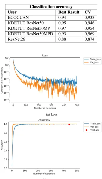
ECOCUAN 0,94 0,933 KDETUT ResNet50 0,95 0,946 KDETUT ResNet50MP 0,97 0,954 KDETUT ResNet50MPD 0,93 0,969 ResNet26 0,88 0,874 (a) Loss (b) Accuracy

Fig. 12: A. Mulgund images+shapes accuracy and loss

see in how much epochs they obtained that accuracy be-cause they obtain 90% of accuracy with few epochs. As we can see in Fig.12, the loss curve is going down, but, the validation accuracy is flat from the beginning. Instead of that, those that do not use these characteristics are classi-fied by the use from 5 to 1 layer in exception of two net-works that doen’t net-works well and they archieve very dif-ferent classification in each running, anantzoid and alutrin are these exceptions. Anantzoiduses an autoencoding ar-chitecture, obtains results from 0.46 to 0.77 on each tables and we think that it is caused because that autoencoding ar-chitecture makes the image small, and then makes upsam-pling making the image to loose too much features. On the other hand,Alutrinuses two Dense layers in the end, one with only 20 neurons, and the last is the classification layer, as he uses only 20 neurons, with the output of 99 classes, we tested it increasing that number to 256 and the classi-fication goes up in ranking, it archieves a 61% accuracy with MEW2012 dataset instead of 57% and setting filter size from 3 to 5 makes accuracy increase to 67%, so fine-tunning the networks will make all the accuracy values of all netoworks to go up. The network ofchurandyneeded

more than 700 epochs to reach that level of accuracy but it must be said that this network is better than the others be-cause with only two layers it is able to archieve better accu-racy than the others, although it needs to much epochs for learning, that network only uses images for training. The difference of this network with the others is that it resizes the images to 64x64 pixels and its first convolutional layer uses 16 neurons instead of 8 that uses the others of the 2-layer networks, and the Dense 2-layer before the classifica-tion only uses 128 neurons when the others uses from 512 to 4096. We think that the important part of the network is the first one, because it is the layer that seed the first inter-esting feature, and the last Dense before the softmax layer is important to have more neurons that the softmax layer, but it is not necessary too much neurons using our black and white datasets. Churandy also includes a 50% dropout right after the first maxpooling, being a good method to prevent overfitting.

Fig. 13: Loss Decrease of numerical trained network

As we can see in Fig. 13, if we see the performance of loss variance we can know if the network can learn more or it arrived to its local minimum. That is the method we used to know if train for more epochs or not. In that image we can see that the best loss is in the 60th epoch and then it begins to increase so it is not necessary to continue training because its best model is in that point. Althoug in 200th epoch it seems that it is beginning to decrease, so if we will we can continue the training over 300 epochs to see what happens.

In table 2 we have the results with only features training. The results are better than only with images or even with images. As explained before, that is because the shapes is a numerical feature, and it is exclusive of each leaf and be-cause of that the model can train better to classify them. But with that networks we can not train with images because the number of neurons in each layer is too big so the memory gets full quickly.

In table 3 we show the results of the networks training with MEW2012 dataset. We can see that the classification is like the table 1 result, since the classification order is in layer criterion. The difference of the results with the Kagge dataset is because the number of classes of each dataset. Kaggle dataset has the quercus class, that has 32 types of it, but they are so similar between them so is you see the Fig.14 we can see 16 classes misclassified and that is the reason for a bad accuracy levels, since the results with MEW2012 dataset are better because that dataset only has 6 quercus classes, so although it could misclassify all the

classes it will be better than Kaggle dataset classification. We tested it training our network with 300x300 kaggle im-ages instead of 96x96 imim-ages that the network uses normaly and we archieved better results obtaining a misclassification of 10 classes instead of 16 so we can say that it is better to train with bigger images.

So, the top network of all the rankings is the AlexNet type ofPhilip Xue, it has the best accuracy in every dataset, in exception of Flaviabw that churandy surpasses him, but with a difference of only 5%. Comparing it with the same implementation of Philip Xue but LeNet style, that has fewer layers, it gets better classification as expected, be-cause AlexNet is the evolution of LeNet. This network is almost like AlexNet network because it not runs on two threads, but it is the actual implementation with keras of that AlexNet architecture.

Followed by A.thakur that uses an image resize at 128x128 and 3 convolutional layers of 32,32 and 64 neu-rons, but reduce the filter size to 3x3 on each layer, although that, they succeed in positioning them in the best places of the rankings and is the only network that has that results in less epochs.

Churandyis the next classificated that with only 2 layers network archieves the third best position. It is because they finetuned very well its network doing more small resize of the image and setting up the number of neurons in only the needed for that type of dataset.

Alutrinalthough it uses 4 layers, gets the worst classi-fication in the rankings because its last Dense layer before the classification layer only uses 20 neurons. Being less than the number of classes in the database, as mentioned above, we trained with more neurons and we obtained bet-ter results, although not enough to go up a lot in the ranking. AndAnantzoidis a particular case that using the autoen-coding method, randomly archieves best or worse results.

The other contestants uses 1 or 2 convolutonal layers but their networks are so similar so they archieve the medium places in the rankins.

Fig. 14: Quercus type classification

You can find the quercus classification example in the annex.

ECOCUAN, KDETUT and ResNet26 In table 6 we can observe the results obtained with the three papers. We can see that the ResNet26obtains the worst result with 88% of accuracy, as we expected, because it has half layers than ResNet50. ECOCUAN team obtains 94% of accu-racy. It is a very good result because they use a network like AlexNet with 5 convolutional layers, so comparing it with the results obtained with ResNet50 the difference is 1% only. It happens because the dataset used in training, as the images are leaf only without background.KDETUT

obtains their best result with ResNetMPD network, as they describe in their paper. The difference between ResNet50 and ResNet50MPD is good enought to say that is the best option to use for classification of leaves. In their paper they use ImageClef dataset, that has leaves, branches, flowers and all the images have background and they obtain good classification results with ResNet50MPD. So it is better to add a Maxpooling layer after the first of the convolutional layers of each bottleneck group. To test the network per-formance with different kernel initializers we tested it with ResNet26 network training for 500 epochs. In Fig.15 we can see the results. Glorot uniformis the initializer that Keras uses by default and if we change it to other initializers we can see that usingOne, Zero or Constant initializers are the worst options to use, but usingRandom uniform or Truncated normalwe obtain best results with a differ-ence of 3% accuracy.

Fig. 15: Initializers

8

CONCLUSIONS

W

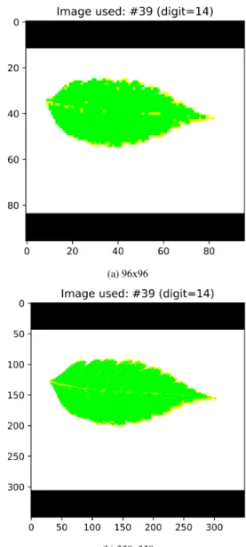
Ehave come to the conclusion that the size of the input image is something to take into account, because we obtained bests results with bigger sizes. Also it is important to set up well each layer of our network, setting the filter sizes taking into account the input size. In our datasets, except in Flavia, it is not very im-portant the size of the input because they are thresholded images, so when resizing them we not lose many features, but in Flavia dataset, being in color, if we reduce the image we lose so much information about the edges and internal venation as we can see in Fig.16. We can see the differ-ence between the two images since the edges on small size are big and distorted, and the venation is practically lost, but in the high resolution image we can see the edges more accurated and the internal venation is in there.

(a) 96x96

(b) 350x350

Fig. 16: Images of Flavia leaf with normalization applied

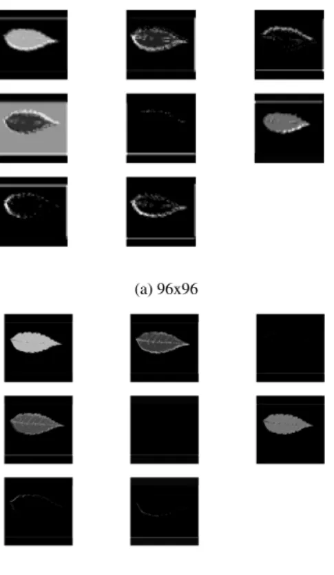
Another example of the importance of resolution is in the layer visualization proccess, as we can see in Fig.17 each neuron saw different characteristics of the leaf, one sees the venation and another edges, but the only think that we can see about high resolution that is worse than with low resolution is that in some layers, the leaf is practically gone, but it is counterbalanced by using the neuronal network that they will make the correct connections to obtain the best classification.

Using our simple images datasets in leaves recogni-tion we obtained a best result with 97% accuracy with ResNet50MPD network so we can confirm that that net-work is the best option for leaf classification, but we are planning to use bigger and with so many types and classes of plants dataset, for example, the ImageClef dataset that contains trusted and noisy data about leaves, branches, flowers and other label informations about the plant in 100gb of data. We will test ResNet50MPD to see if we can obtain the same result as KDETUT team in PlantClef 2017 challenge when they obtained 85,3% accuracy with that network.

We have to take into account how we are going to initial-ize our network, because changing initialinitial-izers can make our

(a) 96x96

(b) 350x350

Fig. 17: First hidden layer visualization

network obtain better results in less time since it is better not to initialize with Zero initializer because we will begin to train in the worst position for the loss function.

Also we learn that it is very important to have the best equipment to train because with a normal Nvidia card the time to train will be so high but with Nvidia Titan and a good CPU and RAM we can obtain results in less than a second with Kaggle networks and in 10 seconds with the pa-per networks. We have an Intel Xeon(R) CPU E5-1620 v4 3.50GHz x 8, with 64GB RAM and Nvidia TITAN GPU. It is true that learning time depends on making batches of the images, with high number the better the results are, but that also makes the learning curves to jump on each epoch and it is worst to see if our network arrived to the minimum or not. You can see an example in Fig.18.

Fig. 18: Batches jumps

Maybe the more difficult of our research is about learn-ing about how a convolutional layer and Maxpoollearn-ing layer works and to know what is the network learning about each image. For example in ECOCUAN implementation

we have a problem making the cross validation because it makes our graphic card to get full and stop, and the problem was in the maxpooling layer filter size because setting it in the best size will make the characteristics be the necessary only with slim size that doesn’t make our net to explode.

9

FUTURE

WORK

T

HANKS to that work we think that the best way to classify leaves is to use ResNet50MP and make it learn the three features splitting the input image in three. For the shape of the leaf making the threshold will work good. For obtain the shape of the leaf will be very difficult as we will have to think the best way to leave the venation of the leaf visible and hide all the other. And for the third feature, we think it will be good to obtain the color of the leaf, as they are so many types with different colors, it will be a good point to separate the classes. We will con-tinue to learn about the best option to classify leaves, but as seen in ImageClef competition, the world of Leaf clas-sification has arrived to its end, with 96% of accuracy it is better to change to another challenge to improve with deep learning. Although we will test our implementations with ImageClef and ImageNet dataset to test our results in a bet-ter way with huge dataset with many types of data. Also we will test the performance of the learning transfer, doing a little research about classifying minerals.

10

A

CKNOWLEDGMENTS

We thank Fernando Vilari˜no for lend us the Nvidia Titan and the CPU used in the research, and for supporting us with all the questions that appears during the research. Without his help all the research would not have been possible. Also we thank Siang Thye Hang and Masaki Aono of the KDE-TUT team for answering us a question about their paper, and sharing the architecture of their network with us.

11

BIBLIOGRAPHY

REFERENCES

[1] The Home of Data Science & Machine Learning. https://www.kaggle.com/c/leaf-classification

[2] ImageCLEF - The CLEF Cross Language Image Retrieval Track. http://www.imageclef.org/lifeclef/2017/plant

[3] Middle European Woods (MEW 2012 and 2014). http://zoi.utia.cas.cz/download

[4] Wu, S. G., Bao, F. S., Xu, E. Y., Wang, Y. X., Chang, Y. F., & Xiang, Q. L. (2007, December). A leaf recog-nition algorithm for plant classification using proba-bilistic neural network. InSignal Processing and In-formation Technology, 2007 IEEE International Sym-posium on(pp. 11-16). IEEE.

[5] LeCun, Y., Bottou, L., Bengio, Y., & Haffner, P. (1998). Gradient-based learning applied to document recognition.Proceedings of the IEEE, 86(11), 2278-2324.

[6] ImageNet Large Scale Visual Recognition Challenge (ILSVRC). http://image-net.org/challenges/LSVRC/ [7] Krizhevsky, A., Sutskever, I., & Hinton, G. E. (2012).

Imagenet classification with deep convolutional neural networks. InAdvances in neural information process-ing systems(pp. 1097-1105).

[8] Zeiler, M. D., & Fergus, R. (2014, September). Vi-sualizing and understanding convolutional networks. InEuropean conference on computer vision(pp. 818-833). Springer, Cham.

[9] Szegedy, C., Liu, W., Jia, Y., Sermanet, P., Reed, S., Anguelov, D., ... & Rabinovich, A. (2015, June). Go-ing deeper with convolutions. Cvpr.

[10] Simonyan, K., & Zisserman, A. (2014). Very deep convolutional networks for large-scale image recog-nition.arXiv preprint arXiv:1409.1556.

[11] He, K., Zhang, X., Ren, S., & Sun, J. (2016). Deep residual learning for image recognition. In Proceed-ings of the IEEE conference on computer vision and pattern recognition(pp. 770-778).

[12] Apple. Build more intelligent apps with ma-chine learning. https://developer.apple.com/mama-chine- https://developer.apple.com/machine-learning/

[13] Cirad, Inra, Inria, IRD, Floristic and Agropolis Fun-dation. Pl@ntNet. http://plantnet.org

[14] Affouard, A., Go¨eau, H., Bonnet, P., Lombardo, J. C., & Joly, A. (2017, April). Pl@ ntNet app in the era of deep learning. InICLR 2017 Workshop Track-5th In-ternational Conference on Learning Representations.

[15] Anaconda Cloud. Where packages, note-books, projects and environments are shared. https://anaconda.org

[16] Franc¸ois Chollet. Keras: The Python Deep Learning library. https://keras.io

[17] ImageNet: Image dataset organized according to the WordNet hierarchy. http://www.image-net.org/ [18] Scikit-learn Machine Learning in Python.

http://scikit-learn.org/stable/

[19] Reyes & A. K., & Caicedo J. C., & Camargo J. E. (2015, September). Fine-tuning Deep Convolutional Networks for Plant Recognition. In CLEF (Working Notes)

[20] Hang, S. T., & Aono, M. (2017). Residual Network with Delayed Max Pooling for Very Large Scale Plant Identification. InWorking Notes of CLEF, 2017

[21] Sun, Y., Liu, Y., Wang, G., & Zhang, H. (2017). Deep Learning for Plant Identification in Natural Environ-ment. Computational intelligence and neuroscience, 2017.

[22] Draw convnets. https://github.com/gwding/draw convnet

[23] Abhijeet Mulgund. Keras ConvNet LB 0.0052 w/ Visualization. https://www.kaggle.com/abhmul/keras-convnet-lb-0-0052-w-visualization.

[24] Aditya Thakur. Processing Image Data into Keras. https://www.kaggle.com/astvd3/processing-image-data-into-keras/code

[25] Alex Lazarev. Simple keras 1d CNN + features split. https://www.kaggle.com/alexanderlazarev/simple-keras-1d-cnn-features-split/code.

[26] Alutrin. Simple CNN leaves with features plugged in later. https://www.kaggle.com/alutrin/simple-cnn-leaves-with-features-plugged-in-later/code.

[27] Anantzoid. Kaggle leaf classification.

https://github.com/anantzoid/Kaggle-Leaf-Classification.

[28] Churandy. Leaf CNN with image generator. https://www.kaggle.com/angelmm/leaf-cnn-with-image-generator/code.

[29] Philip Xue. Leaf classification using CNN. https://www.kaggle.com/philipxue/leaf-classification-using-cnn/code.

[30] Volodymyr Liunda. Leaves classification with convnet in keras wip. https://www.kaggle.com/wolterlw/leave-classification-with-convnet-in-keras-wip/code. [31] Yu-Weichang. Keras model usage on leaf

classi-fication. https://www.kaggle.com/ernie55ernie/keras-model-usage-on-leaf-classification/code.

[32] Picubeisnot30. Merged keras for leaf classification. https://www.kaggle.com/icecube314/merged-keras-for-leaf-classification/code.

[33] Churandy. Leaf keras 2 layered dnn. https://www.kaggle.com/angelmm/leaf-keras-2layerednn

[34] Gauravjoshi. Leaf classification through keras copy. https://www.kaggle.com/gauravjoshi1986/leaf-classification-through-keras-copy/code

[35] Ibprofin. NN keras. https://www.kaggle.com/mwa259/nn-keras.

[36] Konstantin Tumalevich. Keras. https://www.kaggle.com/userad/keras/code

[37] Michael Semeniuk. Feature extraction v4. https://www.kaggle.com/lorinc/feature-extraction-v4/code.

[38] Prateek. Keras Linear. https://www.kaggle.com/prateekbhat/keras-linear.

12

ANNEX

12.1

Kaggle codes implementation:

12.1.1 CNNs

All the figures used in next are made with a code of gwding[22]

Abhijeet Mulgund[23]: That kaggler used images and shapes to train his network. His network has two convo-lutional layers, each one followed by one Activation and MaxPooling layer. It merge the results of that two convo-lutional layers with the shapes and gives it to two Dense layers as output. He resizes the images to 96x96 pixels and do some data augmentation.

Fig. 19: Albhijeet Architecture

Aditya Thakur[24]: That Kaggler used only the images provided. His network has three convolutional layers, each one followed by one Activation and Maxpooling layers, and two Dense layers at the end. He resizes the images to 128x128.

Fig. 20: Aditya Architecture

Alex Lazarev[25]: That Kaggler used only the shapes provided. His network has one convolutional layer followed by one Activation layer, and three Dense layers at the end.

Fig. 21: A. Lazarev Architecture

Alutrin[26]: That Kaggler used only the images pro-vided. His network has four convolutional layers, each one followed by one Maxpooling layer, and one ZeroPadding layer and another MaxPooling layer and gives the results to two Dense layers at the end. He resizes the images to 96x96.

Fig. 22: Alutrin Architecture

Anantzoid[27]: That Kaggler used the images and the shapes provided. His network has four convolutional lay-ers, each one followed by one Maxpooling layer, then an-other four convolutional layers followed by one Upsam-pling layer and then merge the results with the shapes and gives it to four Dense layers at the end. It is called ”autoen-coding”. He resize the images to 128x128.

Fig. 23: Ananzoid Architecture

Churandy[28]: That Kaggler used only the images pro-vided. His network has two convolutional layers, each one followed by one Activation and Maxpooling layers, and two Dense layers at the end. He resize the images to 64x64 and apply some data augmentation.

Fig. 24: Churandy Architecture

Philip Xue[29]: That Kaggler used only the images pro-vided. He says that his first approach to a CNN was us-ing the AlexNet model, but because the time that his CPU needed to learn he decided to change to a most simple LeNet architecture. His LeNet network, Fig.25 has two convolutional layers, each one followed by one Activation and Maxpooling layers, and three Dense layers at the end. His AlexNet network, Fig.25 has five convolutional layers inserting some MaxPooling layers after the first, the second and the fifth layers, and then gives the result to three Dense layers. He resize the images to 96x96.

Fig. 25: Philip LeNet Architecture

Fig. 26: Philip AlexNet Architecture

Volodymyr Liunda[30]: That Kaggler used only the im-ages provided. His network, Fig.27, has one convolutional layers followed by one Maxpooling layer and two Dense layers at the end. He resize the images to 96x96.

Fig. 27: Volodimyr Architecture

Yu Weichang[31]: That Kaggler used the images and shapes provided. His network, Fig.28, merge two models, the first model has one Dense layer that process the shapes, and the second model has one convolutional layer followed by one Activation and Maxpooling layers, then gives the results to two Dense layers. He resize the images to 96x96. The next Kagglers only used the shapes provided, so their neural networks are not Convolutional Networks, but for informational purposes we decided to make a ranking with them.

12.1.2 Only features DNN

We only make the image of network architecture of CNNs because the structure of a DNN is only the fully connected layers.

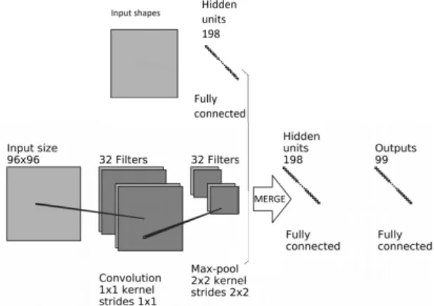
Picubeisnot30[32]: His network is a merge of three mod-els, one for each shape. They has two Dense layers and gives the results merged to another two Dense layers.

Churandy[33]: His network has three Dense layers, one with 800 neurons, another with 200 and the last with 99

Fig. 28: Yu Weichang Architecture

(classes). He perform a Dropout after each Dense layer to avoid overfitting.

Gauravjoshi[34]: His network has three Dense layers, one with 1024 neurons, another with 512 and the last with 99 (classes). He perform a Dropout after each Dense layer to avoid overfitting.

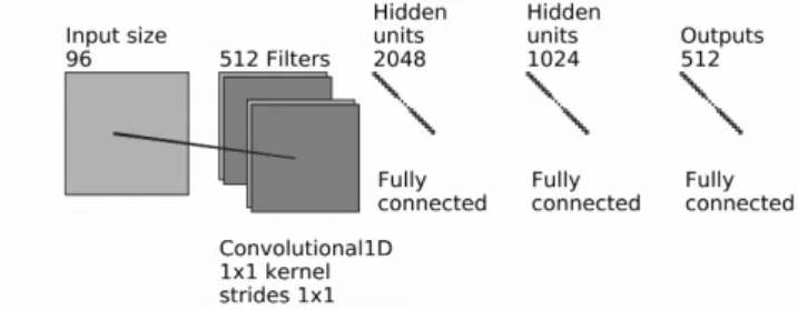
Ibprofin[35]: His network has three Dense layers, one with 2048 neurons, another with 1024 and the last with 99 (classes). He perform a Dropout after each Dense layer to avoid overfitting.

Konstantin Tumalevich[36]: His network has three Dense layers, one with 1024 neurons, another with 512 and the last with 99 (classes). The difference between Kon-stantin and Gauravjoshi is that KonKon-stantin uses ’tahn’ ac-tivation parameter in the first Dense layer. He perform a Dropout after each Dense layer to avoid overfitting.

Michael Semeniuk[37]: His network is a merge of three models, one for each shape. The three models have one Dense layer and merge the outputs and gives them to four Dense layers, two with 120 neurons, and two with 99 (classes). He perform a Dropout after each Dense layer to avoid overfitting.

Prateek[38]: His network has four Dense layers, one with 192 neurons(quantity of numbers in a shape), two with 120 and the last with 99 (classes). He perform a Dropout after each Dense layer to avoid overfitting.

12.2

Classification report example of quercus

classification: