Lehigh University
Lehigh Preserve
Theses and Dissertations
2016
Randomized Algorithms for Nonconvex
Nonsmooth Optimization
Xiaocun Que
Lehigh University
Follow this and additional works at:
http://preserve.lehigh.edu/etd
Part of the
Industrial Engineering Commons
This Dissertation is brought to you for free and open access by Lehigh Preserve. It has been accepted for inclusion in Theses and Dissertations by an authorized administrator of Lehigh Preserve. For more information, please [email protected].
Recommended Citation
Que, Xiaocun, "Randomized Algorithms for Nonconvex Nonsmooth Optimization" (2016).Theses and Dissertations. 2774.
Randomized Algorithms for Nonconvex Nonsmooth
Optimization
by
Xiaocun Que
Presented to the Graduate and Research Committee of Lehigh University
in Candidacy for the Degree of Doctor of Philosophy
in
Industrial Engineering
Lehigh University January 2016
c
Copyright by Xiaocun Que 2016 All Rights Reserved
Approved and recommended for acceptance as a dissertation in partial fulfillment of the requirements for the degree of Doctor of Philosophy.
Date
Dissertation Advisor
Committee Members:
Frank E. Curtis, Committee Chair
Michael L. Overton
Katya Scheinberg
Acknowledgements
First, I would like to thank my advisor Prof. Frank E. Curtis for his excellent guidance during my Ph.D. years. Second, I would like to thank the members of my dissertation committee, Prof. Michael L. Overton, Prof. Katya Scheinberg, and Prof. Ted K. Ralphs, for their insightful questions, comments, and suggestions. Third, I would like to thank the Computational Optimization Research Lab (COR@L) in the Industrial and Systems Engineering (ISE) Department at Lehigh University, because most of the numerical exper-iments presented in this thesis were performed using software and hardware in COR@L. Fourth, I would like to thank the National Science Foundation (NSF), because this work was financially supported in part by NSF grant DMS-1016291. Finally, I would like to thank my husband Xiong Xiong for his continuous support since we got married.
Contents
Acknowledgements iv
List of Tables viii
List of Figures ix Abstract 1 1 Introduction 3 1.1 Theoretical Background . . . 5 1.2 Classical Algorithms . . . 7 1.2.1 Subgradient Method . . . 7
1.2.2 Cutting Plane Method . . . 9
1.2.3 Proximal Point Method . . . 10
1.2.4 Bundle Method . . . 11
1.2.5 Gradient Sampling Method . . . 14
1.2.6 Smoothing Method . . . 18
2 An Adaptive Gradient Sampling Algorithm 21 2.1 Introduction . . . 22
2.2 Algorithm Description . . . 24
2.3 Hessian Approximation Strategies . . . 27
2.3.1 LBFGS Updates on Sampled Directions . . . 28
2.4 Global Convergence Analysis . . . 33 2.5 An Implementation . . . 41 2.5.1 Algorithm Variations . . . 41 2.5.2 Test Problems . . . 44 2.5.3 Numerical Results . . . 44 2.6 Conclusion . . . 47
3 A BFGS Gradient Sampling Algorithm 49 3.1 Introduction . . . 49
3.2 Algorithm Description . . . 53
3.2.1 Main Algorithm . . . 54
3.2.2 Line Search . . . 59
3.2.3 Sample Point Generation . . . 62
3.2.4 Hessian Approximation Strategy . . . 64
3.3 Global Convergence Analysis . . . 69
3.4 Implementation and Numerical Experiments . . . 77
3.4.1 An Implementation and Alternative Software . . . 77
3.4.2 Test Problems . . . 80
3.4.3 Numerical Results . . . 82
3.5 Conclusion . . . 87
4 Algorithmic Extensions 89 4.1 A Bundle Gradient Sampling Algorithm . . . 89
4.1.1 Algorithm Description . . . 92
4.1.2 Global Convergence Analysis . . . 94
4.1.3 Numerical Experiments . . . 101
4.2 A Smoothing BFGS Gradient Sampling Algorithm . . . 102
4.2.1 Algorithm Description . . . 103
4.2.2 Global Convergence Analysis . . . 105
4.3 Gradient Sampling for`1-Regularization . . . 115
4.3.1 Algorithm Description . . . 115
4.3.2 Global Convergence Analysis . . . 118
4.3.3 Numerical Experiments . . . 123
5 Conclusion 125
Bibliography 127
A QO Subproblem Solver 133
B Nonsmooth Test Problems 137
List of Tables
2.1 Summary of six algorithm variations used to test the adaptive sampling procedure in Algorithm 4 along with the Hessian approximation updating
strategies described in§2.3.1 and §2.3.2. . . 42
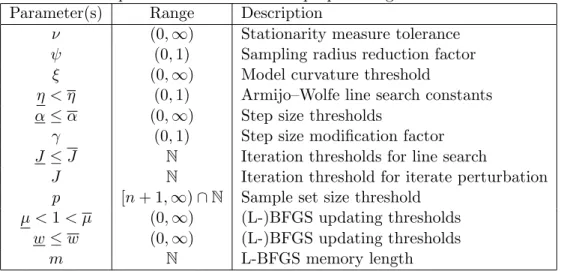
3.1 User-specified constants for the proposed algorithm and subroutines . . . . 54
3.2 Summary of input parameters for algorithmbfgs-gs. . . 78
3.3 Counts of termination flag types . . . 84
3.4 For each solver and each test problem, the geometric means of stationarity measures . . . 88
4.1 User-specified constants for the proposed algorithm . . . 105
4.2 Results for prostate cancer from algorithmSBFGSGS . . . 112
4.3 Results for prostate cancer from algorithmSTR . . . 112
4.4 Results for prostate cancer with penalty functionφ3 from algorithmSBFGSGS113 4.5 Results for prostate cancer with penalty functionφ3 from algorithm STR . . 113
4.6 Results of linear regression from algorithmSBFGSGS . . . 115
4.7 Results of linear regression from algorithmSTR . . . 116
4.8 Results of logistic regression from algorithmSBFGSGS . . . 117
4.9 Results of logistic regression from algorithmSTR . . . 117
List of Figures
1.1 Illustration of the Bundle Method. . . 14
1.2 Illustration of the Gradient Sampling Algorithm. . . 18
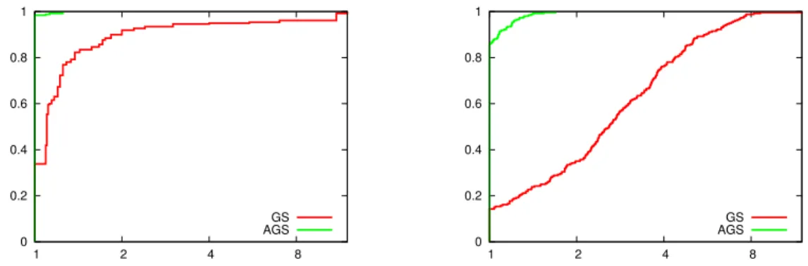
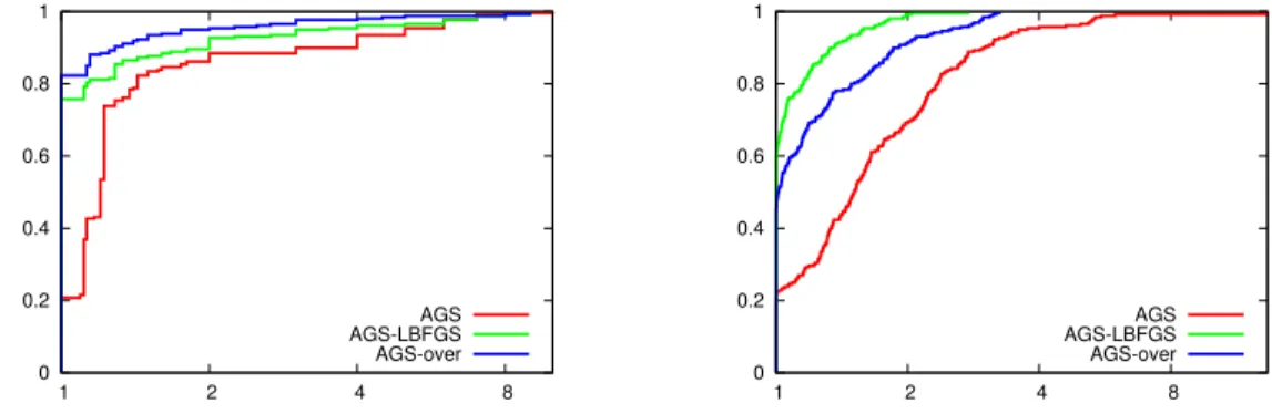
2.1 Performance profiles for the final sampling radius (left) and average QO iterations per nonlinear iteration (right) comparing algorithmsGSand AGS. 45 2.2 Performance profiles for the final sampling radius (left) and average QO iter-ations per nonlinear iteration (right) comparing algorithmsAGS,AGS-LBFGS, andAGS-over. . . 46
2.3 Performance profiles for the final sampling radius (left) and average QO iterations per nonlinear iteration (right) comparing algorithmsAGS-LBFGS, AGS-LBFGS-ill,AGS-overand AGS-over-ill. . . 47
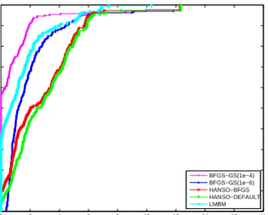
3.1 Performance profile for iterations . . . 85
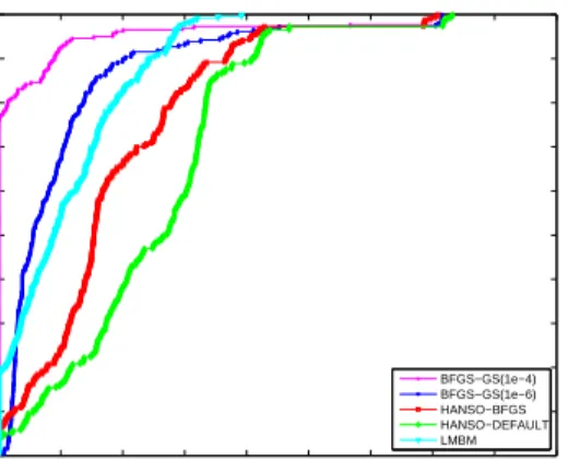
3.2 Performance profile for function evaluations . . . 85
3.3 Performance profile for gradient evaluations . . . 86
4.1 Illustration of bundle sampling method. . . 92
4.2 Performance profiles for nonlinear iterations (upper left), function evalua-tions (upper right), gradient evaluaevalua-tions (lower left), and overall QO itera-tions (lower right) comparing algorithmsAGSand BGS. . . 103
4.3 Illustration of the gradient matrixG1k. . . 118
Abstract
Nonsmooth optimization problems arise in a variety of applications including robust con-trol, robust optimization, eigenvalue optimization, compressed sensing, and decomposition methods for large-scale or complex optimization problems. When convexity is present, such problems are relatively easier to solve. Optimization methods for convex nonsmooth optimization have been studied for decades. For example, bundle methods are a leading technique for convex nonsmooth minimization. However, these and other methods that have been developed for solving convex problems are either inapplicable or can be ineffi-cient when applied to solve nonconvex problems. The motivation of the work in this thesis is to design robust and efficient algorithms for solving nonsmooth optimization problems, particularly when nonconvexity is present.
First, we propose an adaptive gradient sampling (AGS) algorithm, which is based on a recently developed technique known as the gradient sampling (GS) algorithm. Our AGS algorithm improves the computational efficiency of GS in critical ways. Then, we propose a BFGS gradient sampling (BFGS-GS) algorithm, which is a hybrid between a standard Broyden-Fletcher-Goldfarb-Shanno (BFGS) and the GS method. Our BFGS-GS algorithm is more efficient than our previously proposed ABFGS-GS algorithm and also competitive with (and in some ways outperforms) other contemporary solvers for nons-mooth nonconvex optimization. Finally, we propose a few additional extensions of the GS framework—one in which we merge GS ideas with those from bundle methods, one in which we incorporate smoothing techniques in order to minimize potentially non-Lipschitz objective functions, and one in which we tailor GS methods for solving regularization prob-lems.
We describe all the proposed algorithms in detail. In addition, for all the algorithm variants, we prove global convergence guarantees under suitable assumptions. Moreover, we perform numerical experiments to illustrate the efficiency of our algorithms. The test problems considered in our experiments include academic test problems as well as practical problems that arise in applications of nonsmooth optimization.
Chapter 1
Introduction
This dissertation involves a study of the minimization of locally Lipschitz objective func-tions that may be both nonsmooth and nonconvex. Problems of this type arise in a variety of applications including robust control [27, 28, 58, 59], robust optimization [3, 23, 60], eigenvalue optimization [1], compressed sensing [12, 20], and decomposition methods for large-scale or complex optimization problems [5, 52]. Solutions of such problems often lie at points of nondifferentiability of the objective. This makes it imperative to design robust and efficient algorithms for the optimization of nonsmooth functions.
A variety of algorithms have been proposed for nonsmooth optimization. Many, how-ever, are based on the assumption that the objective function is convex. For example, bundle methods [34], which rely on the ability to produce linear underestimators of the objective (i.e., cutting planes) are a leading technique for convex nonsmooth minimization. There are extensions to traditional bundle methods for solving nonconvex problems, but these methods are complex and we believe that alternative strategies may be better suited for handling nonconvexity.
The goal of the research outlined in this thesis is to develop, analyze, and implement efficient methods for solving nonsmooth optimization problems, particularly when non-convexity is present. We study and propose extensions for a recently developed technique known as the gradient sampling (GS) algorithm [9, 39]. In contrast to bundle methods, GS handles nonconvexity without any extra algorithmic modifications, which makes it
an attractive starting point for devising new methods for nonconvex optimization. The methods that we propose also incorporate quasi-Newton strategies, for which many have observed good practical performance, even when they are applied to solve nonsmooth problems [44].
After providing theoretical background on nonconvex optimization problems and algo-rithms that have been proposed for solving them, we begin the main part of this thesis by describing research that addresses some efficiency issues of GS. In Chapter 2, we propose an adaptive gradient sampling (AGS) algorithm, which improves the computational efficiency of GS by incorporating an adaptive sampling technique and Hessian updating strategies. Our numerical experiments illustrate that AGS outperforms GS in critical ways. In Chap-ter 3, we propose a BFGS Gradient Sampling (BFGS-GS) Algorithm, which is a hybrid between a standard Broyden-Fletcher-Goldfarb-Shanno (BFGS) and the GS method. The algorithm has been implemented in C++ and the results of numerical experiments are presented to illustrate the efficacy of the proposed numerical method.
The remainder of the thesis considers further extensions to the GS framework. In particular, in Chapter 4.1, we propose a bundle gradient sampling (BGS) algorithm that merges GS strategies with those of bundle methods so that the overall approach remains effective for convex problems and does not require algorithmic modifications to handle nonconvexity. We combine the two strategies into a single “bundle sampling” framework, provide theoretical convergence guarantees that are on par with those currently held by GS, and provide the results of numerical experiments to illustrate the computational per-formance of our new method. In Chapter 4.2, we propose a smoothing BFGS gradient sampling algorithm, which is based on the smoothing method and our BFGS-GS algorithm for nonsmooth optimization. A motivation for the smoothing approach is that it has the-oretical convergence guarantees even when the problem functions are not Lipschitz. (This is more than can be said about the other algorithms in the thesis.) Numerical results are presented to illustrate that our algorithm is competitive with another recently proposed smoothing method for non-Lipschitz optimization. In Chapter 4.3, we tailor GS methods to solve regularized problems. Global convergence analysis is provided. Preliminary
nu-merical experiments are performed to compare different algorithmic variations of GS with another algorithm proposed for solving regularization problems.
1.1
Theoretical Background
In this section, we provide essential definitions and background for the study of minimizing nonsmooth functions. We also outline notation that will be used throughout the thesis.
We consider the unconstrained problem
min
x∈Rn f(x) (1.1)
where f : Rn → R is locally Lipschitz and continuously differentiable in an open dense
(see below) subset D of Rn. A function f :Rn → R is Lipschitz continuous [49] if there
exists a constant L >0 such that
kf(x)−f(y)k2 ≤Lkx−yk2 (1.2)
for all x, y∈Rn. The constantL is called the Lipschitz constant which is independent of
x and y. There are a variety of convenient features of Lipschitz continuous functions. In short, a Lipschitz continuous function is limited in how fast it can change. Also, for any two points on the graph of a Lipschitz continuous function, the absolute value of the slope of the line joining those two points is bounded above by a constant. Given a particular point x, a function f : Rn → R is locally Lipschitz continuous [49] at x ∈ Rn with a
constantL >0 if (1.2) holds for all y and z in a neighborhood ofx.
A subsetD ofRn is called dense [57] if any neighborhood of x∈Rn contains at least
one point in D. Note that this means that the closure of D is Rn and that the interior
of the complement of D is the empty set. An important consequence of our assumption that f is continuously differentiable in such a set Dis that there exist points at which f
is differentiable in any arbitrarily small neighborhood of a given point x.
for deriving optimality conditions for problem (1.1). We define the Euclidean-ball about
x to be
B(x) :={x:kx−xk2≤}. (1.3)
Moreover, let cl convS denote the closure of the convex hull ofS⊆Rn. The multifunction
G(x) := cl conv∇f(B(x)∩ D) (1.4)
can then be seen as the closure of the convex hull of the gradients at all the points in the intersection of an -ball about x and the set D in which f is differentiable. Given these definitions, the Clarke subdifferential [15] of f atx can be expressed as the following:
∂f(x) = \
>0
G(x).
A point x is stationary forf if 0 ∈∂f(x). The gradient sampling algorithm discussed in detail later on in this thesis makes use of an extension to the subdifferential, namely the
-subdifferential introduced by Goldstein [24]. The Clarke -subdifferential is given by
∂f(x) := cl conv∂f(B(x)),
andxis-stationary if 0∈∂f(x). Observe from this definition that a reasonable strategy
for computing a stationary point for f is to compute a sequence of-stationary points for
→0.
As previously mentioned, we are interested in the minimization of nonsmooth func-tions that may also be nonconvex. We do, however, make extensive comments pertaining exclusively to convex functions, and it is important to distinguish definitions of quantities that suppose convexity. A function f :Rn→R is convex [53] if
f(λx+ (1−λ)y)≤λf(x) + (1−λ)f(y)
the function lies below the line segment joining any two points of the graph. It is known that a real-valued convex function is guaranteed to be locally Lipschitz continuous at any
x. Moreover, the subdifferential of a convex functionf atx is the set
∂f(x) ={g∈Rn |f(y)≥f(x) +gT(y−x) ∀y∈Rn}.
Each vector g∈∂f(x) is called asubgradient [53] off atx.
1.2
Classical Algorithms
The nondifferentiability of the objective functionf in (1.1) excludes the direct application of smooth gradient-based algorithms. Therefore, in this section we introduce some basic methods for solving nonsmooth optimization problems: the subgradient method, cutting plane method, proximal point method, bundle method, gradient sampling method, and smoothing method. For the first four algorithms in this section, note that all rely on the assumption thatf is convex. This is important as, later on, we aim to design algorithms that do not make this assumption. Our descriptions of the first four algorithms in this section are based on the descriptions in [53]. The description of the gradient sampling (GS) method is based on the description in [9] and [39]. The description of the smoothing method is based on the description in [13].
1.2.1 Subgradient Method
As the gradient descent method is the most basic algorithm for smooth differentiable optimization, the subgradient method is the most basic method for nonsmooth problems. The approaches are nearly identical, but the idea behind the subgradient method is to replace the gradient of f at x with any arbitrary subgradient. Given an iterate xk, an
iteration of the subgradient method is given by
where gk∈∂f(xk) is a subgradient off atxk and αk is a positive step size.
There are some serious drawbacks of the subgradient method. First, note that a negative subgradient direction gk is not necessarily a direction of descent of f from xk.
Therefore, under various step size selection rules, the sequence {f(xk)} in subgradient
methods is not guaranteed to be nonincreasing. Moreover, some standard line search techniques (e.g., the Armijo or Wolfe conditions [49]) cannot be applied for choosing αk.
There are certain step size selection rules that do guarantee global convergence of the method, but in many cases these rules are important only for their theoretical significance and are rarely used in practice due to their low efficiency. The key property of the subgradient method is that a small step in the direction negative to gk will decrease the
distance to the optimal solution set. This fact is used in the proofs of many convergence theorems [53].
Another drawback of the subgradient method is that a theoretically sound and prac-tically robust termination condition is elusive in many applications. For one thing, the norm of an arbitrary subgradient does not necessarily become small in the neighborhood of an optimal point, meaning that termination conditions typical in smooth optimization do not generally apply for nonsmooth problems.
An important special case of the subgradient method is whengkis always chosen to be
the minimum-norm subgradient off atxk. In such cases, gk is always a descent direction
from anyxkthat is not a minimizer off; in particular, it defines the direction of steepest
descent for f from xk. Despite this nice feature, however, one finds that as in smooth
optimization, algorithms based on steepest descent directions can be slow to converge in practice. Moreover, computing the steepest descent direction for a nonsmooth function f
at any point is not always a viable option.
Perhaps the only clear advantage of the subgradient method comes from its simple structure.
1.2.2 Cutting Plane Method
Given an assumption of convexity, the idea behind cutting plane methods is to use sub-gradient inequalities to construct a convex piecewise linear approximation of the objective function at each iterate xk. Specifically, given points {x1, . . . , xk}, suppose that values
of the objective {f(x1), . . . , f(xk)} and subgradients{g1, . . . , gk} have been accumulated
from previous iterations. We can then construct the following lower approximation of f
atxk:
mCPk (x) := max
1≤j≤k{f(xj) +g T
j(x−xj)}. (1.6)
The minimization of the model function (1.6) is called the master problem:
min
x∈Rn
mCPk (x). (1.7)
After solving (1.7), a new iterate xk+1 is obtained. The iterate xk+1, objective value
f(xk+1) and subgradientgk+1 can then be added to the model to construct a new linear
underestimator of f. Each linear piece f(xj) +gTj(x−xj), added at each iteration, is
called a cutting plane (or simply a cut). A key property of the master problem (1.7) is that, due to the convexity of f, its optimal value provides a lower bound for the optimal value of (1.1).
The master problem (1.7) can be written equivalently as the following linear optimiza-tion (LO) problem:
min (x,z)∈Rn× R z s.t. f(xj) +gjT(x−xj)≤z, j = 1, . . . , k. (1.8)
In this formulation, a new constraint is added to the problem after each cutting plane is computed, which means the number of dual variables is increased by one after each iteration. This means that re-optimization by a dual method is an attractive option because it can start with a feasible solution obtained from a previous iteration.
One reason for this is that there exist no reliable rules for removing the old cuts, even when they are inactive at a given solution (1.8). Usually, very many iterations are needed to achieve satisfactory accuracy in the solution. Only in the special case when the objec-tive function is also piecewise linear and convex does the cutting plane method become consistently efficient. Cutting plane methods are important, however, as they form a basis for more effective techniques.
1.2.3 Proximal Point Method
Consider the function
h(w) := min
x∈Rn
f(x) +12kx−wk2 . (1.9)
This is known as the Moreau-Yosida regularization of the objective function f(x). Iff is convex, then it can be shown that h(w) is convex and continuously differentiable. (The Moreau-Yosida regularization is often defined with a positive scalar weighting the proximal term 12kx−wk2. This weight can affect the practical performance of the method, but it is
not necessary for our purposes here or in the subsection on bundle methods below.) The variable w can be thought of as a centering term. The goal of (1.9) is to minimize the true objective f as well as stay close to the center wk. (The reason that we use wk’s as
the iterates instead of the xk’s like we did in previous subsections is that we want to be
consistent with the notation defined in bundle methods, which we will introduce in the next subsection.) In bundle methods, it is necessary to define two sequences: the iterates
xk’s and the centering terms wk’s. The wk’s can also be thought of as the “best iterates
attained so far”.
Using the Moreau-Yosida regularization off(x), the proximal point method constructs the following iterative process. At iteration k, givenwk, the point x(wk) is computed as
the solution of the problem (1.9). This then defines the iterative sequence
wk+1 =x(wk), k= 1,2, . . . . (1.10)
by the construction of the Moreau-Yosida regularization, we have h(wk) ≤ f(wk) if we
plug in a feasible solution x = wk to the problem (1.9) with w = wk. We also have
f(wk+1)≤h(wk) if we notice thatx=x(wk) is the optimal solution to the problem (1.9)
with w =wk. Therefore, we have f(wk+1) ≤ f(wk), k = 1,2, . . ., namely, the sequence
f(wk) is nonincreasing.
The proximal point method has its disadvantages. It does not appear to be very practical, because each iteration involves the solution of the optimization problem (1.9), which is not easy to solve because of the existence of the original objective function f(x) in the objective of (1.9). However, the proximal point method is an important theoretical model of various highly efficient methods such as bundle methods, described next.
1.2.4 Bundle Method
Bundle methods are regarded as very effective and reliable methods for nonsmooth op-timization. The basic idea of bundle methods is to approximate the subdifferential of the objective function by gathering subgradient inequalities from previous iterations into a bundle. This makes them similar to cutting plane methods in that they require the computation of one arbitrary subgradient and the objective value at each new iterate. A critical difference, however, is that the search direction is obtained by solving a specially designed quadratic optimization (QO) problem, not a LO problem. This helps bundle methods avoid some of the disadvantages of a straightforward cutting plane technique.
The bundle method we introduce in this section is a hybrid of the cutting plane method and the proximal point method that were introduced in previous sections. At iteration k, we define the following regularized master problem:
min
x∈Rnm
BM
k (x) + 12kx−wkk
2. (1.11)
This problem is exactly the same as problem (1.9) except that we use a model mBM k (x)
is similar to the model (1.7) defined in the cutting plane method:
mBMk (x) := max
j∈Jk
{f(xj) +gjT(x−xj)}. (1.12)
Here, similar to before, gj ∈ ∂f(xj) are arbitrary subgradients computed during the
iterations in the index setJk ⊂ {1, . . . , k}. We may think ofJkas being equal to{1, . . . , k},
but note that under certain circumstances an index can be removed fromJk(i.e., a cutting
plane can be removed from mBMk ) without adversely affecting the performance of the algorithm.
Let xk+1 be the solution of the regularized master problem (1.11). If the model
mBMk (x) is exact in the sense that mBMk (x) = f(x) for all x ∈ Rn, then (1.11) would
be identical to problem (1.9) defined for the proximal point method. We could then set
wk+1 =xk+1 as in the proximal point method to obtain the newwk+1, and, in this
man-ner, all steps would be descent steps. That is, all steps would be those where the objective function value has decreased. However, due to the fact that mBMk (x) only approximates
f(x), the solution of (1.11) is different than the solution of (1.9). In particularxk+1 may
not even be better than wk in terms of minimizingf. This necessitates defining a
condi-tion under which the estimate of the optimal solucondi-tion (i.e., w) is updated or remains the same.
For this purpose, we introduce a parameterγ used for updatingwk. If the ratio of the
observed improvement in the objective value over the predicted improvement is greater than γ, namely,
f(wk)−f(xk+1)
f(wk)−mk(xk+1)
≥γ, (1.13)
then we set wk+1 := xk+1. This is called a descent step as we obtain f(wk+1) < f(xk).
Otherwise, we set wk+1 :=wk. This is called a null step. Even though the objective has
not improved due to a null step, by the addition of a new cut, it can be shown that the model mBMk+1 is a sufficient improvement over mBMk in that, after a finite number of null steps, a descent step will be produced.
equivalently written as a problem with a quadratic objective function and linear con-straints: min (x,z)∈Rn×R z+12kx−wkk2 s.t. f(xj) +gTj(x−xj)≤z, j ∈Jk. (1.14)
We provide a detailed description of a bundle method as Algorithm 1 below.
Algorithm 1 The Bundle Method
1: (Initialization): Choose a parameterγ ∈(0,1). Choose an initialx0∈ D, setJ−1 ← ∅,
z0← −∞ and k←0.
2: (Bundle addition): Compute f(xk) and gk ∈ ∂f(xk). If f(xk) > zk, then Jk ←
Jk−1∪ {k}; otherwise,Jk←Jk−1.
3: (Step update): If k = 0 or if f(xk) ≤ (1−γ)f(wk−1) +γzk (recall (1.13)), then set
wk←xk; otherwise set wk←wk−1.
4: (Search direction computation): Solve the master problem (1.14) to obtain (xk+1, zk+1).
5: (Stationarity test): If zk+1 =f(wk), then stop; wk is an optimal solution.
6: (Bundle removal): Remove from Jk some (or all) cuts whose Lagrange multipliers at
the solution of the master problem (1.14) are 0.
7: (Iteration increment): Setk←k+ 1 and go to step 2.
We refer to [53] for the following convergence result for BM.
Theorem 1.2.1. Suppose that the objective function f of problem (1.1) is convex and
that problem has an optimal solution. Then, the sequence {wk} generated by the bundle
method converges to an optimal solution of (1.1).
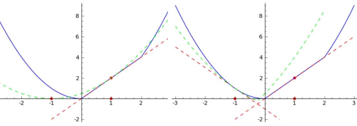
We close this section with an illustrative example of the workings of the bundle method. Consider minimizing the following objective function:
f(x) = max
x∈R
{x2,2x}. (1.15)
Suppose we start with x0= 1. Then we have the following QO subproblem:
min (x,z)∈R×Rz+ 1 2(x−1) 2 s.t.2 + 2(x−1)≤z. (1.16)
left, the red line is the first cut 2 + 2(x−1); the green line corresponds to the objective in an unconstrained reformulation of (1.16). After solving the QO subproblem (1.16), we move to x1 =−1. Then we have the following QO subproblem:
min (x,z)∈R×R z+ 12(x+ 1)2 s.t.2 + 2(x−1)≤z 1−2(x+ 1)≤z. (1.17)
We can see from the plot on the right, another cut 1−2(x+ 1) is added to the plot. After solving (1.17), we move closer to the optimal point. If we continue this process, the bundle method will find the optimal solution.
Figure 1.1: Illustration of the Bundle Method.
1.2.5 Gradient Sampling Method
The original GS algorithm was introduced and analyzed by Burke, Lewis, and Overton [9] for problems of form (1.1). Stronger theoretical results for a slightly revised version of GS were provided in [39], and further extensions have been considered for constrained problems [16] and problems for which only function evaluations are available [40].
The algorithmic structure of GS is very straightforward. At each iteration, we first sample a group of points around the current iterate and evaluate the gradient of f at the current iterate and at the sample points. The search direction is then set as the negative of the vector in the convex hull of the available gradients with smallest norm.
Finally, a backtracking line search is used to obtain a point with a lower objective value. The algorithm starts with an arbitrary positive initial sampling radius, updating it when appropriate to ensure that a stationary point forf is obtained.
More precisely, at a given iterate xk and for a given sampling radius k > 0, the
central idea behind gradient sampling techniques is to approximate Gk(xk) (recall (1.4))
through the random sampling of gradients in Bk := Bk(xk) ∩ D. This set, in turn,
approximates the Clarke k-subdifferential since, at anyx,G(x)⊂∂f(x) for any ≥0
and ∂0f(x)⊂G00(x) for any00 > 0 ≥0. If the computed search direction is large, then
as it is easily shown to be a direction of descent for f, the line search easily produces a new iterate with an improved objective value. Otherwise, by locating xk at which
the minimum-norm element of Gk(xk) is small, reducing the sampling radius, and then
repeating the process fork→0, gradient sampling techniques locate stationary points of
f by successively locating (approximate)k-stationary points for decreasing values ofk.
We now give a detailed description of the GS algorithm. During iterationk, letXk:=
xk∪Xk wherexkis the current iterate andXk :={xk,1, . . . , xk,p}is composed ofp≥n+ 1
points generated independently and uniformly in Bk. With
Gk:= conv{gk, gk,1, . . . , gk,p} (1.18)
defined as the convex hull of the gradients at the points inXk, the search direction is set to
be the negative of the minimum norm vector in Gk, namely,dk=−Proj(0|Gk). This can
be obtained via the solution of a QO problem. Specifically, in order to compare the QO of GS with the QO of AGS and BGS in later sections, we write the QO in a primal-dual form. Let Gk := gk gk,1 · · · gk,p (1.19)
have the following QO subproblem: min z,d z+ 1 2kdk 2 s.t. f(xk)e+GTkd≤ze. (1.20)
Here, edenotes a vector of ones whose length is determined by the context. The dual of (1.20) is given by max π − 1 2kGkπk 2 s.t. eTπ= 1, π ≥0, (1.21)
The solution (zk, dk, πk) of (1.20)–(1.21) has a relationship that dk =−Gkπk.
A specific GS algorithm is presented as Algorithm 2 below.
Algorithm 2 Gradient Sampling (GS) Algorithm
1: (Initialization): Choose a number of sample points to compute each iterationp > n+1, sampling radius reduction factorψ∈(0,1), sufficient decrease constant η∈(0,1), line search backtracking constant κ ∈(0,1), and tolerance parameter ν > 0. Choose an initial iterate x0 ∈ D, set X−1 ← ∅, choose an initial sampling radius 0 >0, and set
k←0.
2: (Sample set update): SetXk ←xk∪Xk, where Xk :={xk,1, . . . , xk,p} 3: (Search direction computation): Setdk ← −Gkπk, whereπk solves (1.21).
4: (Stationarity test): If kdkk ≤ k ≤ ν, then stop. Otherwise, if kdkk ≤ k, then set
xk+1←xk,αk ←1, andk+1 ←ψk and go to step 7.
5: (Backtracking line search): Set αk as the largest value in{κ0, κ1, κ2, . . .} such that
the following sufficient decrease condition
f(xk+αkdk)≤f(xk)−ηαkkdkk2. (1.22)
is satisfied.
6: (Iterate update): Set k+1 ← k. If xk+αkdk ∈ D, then set xk+1 ← xk+αkdk.
Otherwise, set xk+1 as any point in D satisfying the following perturbed line search
conditions
f(xk+1)≤ f(xk)−ηαkkdkk2 (1.23a)
and kxk+αkdk−xk+1k ≤ min{αk, k}kdkk. (1.23b)
7: (Iteration increment): Setk←k+ 1 and go to step 2.
Note that after the search direction dk is computed, a standard backtracking line
search is performed to find a step size αk. We set xk+1 ← xk+αkdk for αk chosen to
be necessary to perturb such an xk+1; see [39] for the motivation of these perturbed line
search conditions and a description of how, given αk and dk satisfying (1.22), an xk+1
satisfying (1.23) can be found in a finite number of operations. The chance seems to be very slim for the algorithm to come to the situation that xk+αkdk∈ D/ . Therefore, while
one may choose to skip this step in practice, it is necessary in establishing convergence guarantees.
The GS algorithm structure is very simple, though its convergence analysis in some-what complicated by the stochastic nature of the algorithm. The convergence result is stated as the following. Please refer to§3 of [39] for the convergence proof.
Theorem 1.2.2. Let {xk} be a sequence generated by GS withν = 0. Then, with
proba-bility 1, Algorithm 2 does not stop, and either f(xk)→ −∞, or k→0 and every cluster
point of {xk} is stationary for f.
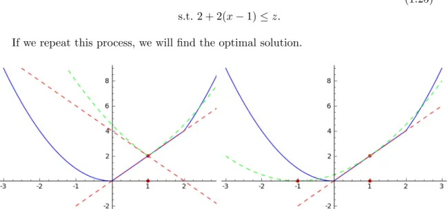
We close this subsection with a description about how GS works on the same example (1.15) we mentioned before. Suppose we start with x0 = 1. Let 0 = 2 be the initial
sampling radius and p = 2 be the number of points sampled per iteration. At k = 0, suppose we generate two pointsx0,1 =−1 andx0,2 = 1.5. Then we have the following QO
subproblem: min (x,z)∈R×R z+ 12(x−1)2 s.t.2 + 2(x−1)≤z 2−2(x+ 1)≤z. (1.24)
The blue curve in Figure 1.2 corresponds to objective (1.15). In the plot on the left, the green line corresponds to the objective in an unconstrainded reformulation of (1.24). After solving the QO subproblem (1.24), we stay at the same point x1 = 1. However, we
shrink the sampling radius 1 = 1. In the plot on the right, if we sample again in the
min
(x,z)∈R×R
z+ 12(x−1)2
s.t.2 + 2(x−1)≤z.
(1.25)
If we repeat this process, we will find the optimal solution.
Figure 1.2: Illustration of the Gradient Sampling Algorithm.
1.2.6 Smoothing Method
The central idea behind a smoothing method is to use a parameterized smooth function to approximate the original nonsmooth objective function. The parameterization of the function is such that, if the smoothing parameter vanishes, then the original function is obtained. On the other hand, with a nonzero smoothing parameter, the given smoothed function can be minimized to produce an approximate minimizer of the original nonsmooth function, where any algorithm for smooth minimization can be used to minimize the smoothed function. By updating the smoothing parameter in an appropriate manner, one can show convergence to a minimizer of the original nonsmooth function.
In the smoothing method, we assume that the parameterized smoothing function sat-isfies the following assumption.
Assumption 1.2.3. Let f : Rn → R be a continuous function with f˜ : Rn ×R+ →
differentiable in Rn for any fixed µ >0, and we have lim z→x,µ→0 ˜ f(z, x) =f(x) for any x∈Rn.
The smoothing method can be constructed by using the function and gradient value of the smoothing function, namely, ˜f and ∇xf˜. We present a description of a specific
smoothing method as Algorithm 3 below.
Algorithm 3 The Smoothing Method
1: (Initialization): Choose a stationarity tolerance parameterν >0, a smoothing param-eter reduction factor ψ ∈ (0,1), an initial iterate x0 ∈ Rn, and an initial smoothing
parameterµ0 >0. Setk←0.
2: (Inner iteration): Solve the following smooth optimization problem approximately to obtain an approximate solutionxk+1:
min
x
˜
f(x, µk)
3: (Outer iteration): If k∇xf˜(xk+1, µk)k ≥ νµk, then setµk+1 ← µk; otherwise, choose
µk+1 ←ψµk.
4: (Iteration increment): Setk←k+ 1 and go to step 2.
We refer to [13] for the following convergence result for the smoothing method.
Theorem 1.2.4. The smoothing method produces an infinite sequence of iterates {xk}
and either for some µk >0we have f˜(xk, µk)→ −∞or {µk} →0 and every cluster point
of {xk} is stationary for f.
The advantage of the smoothing method is that we can make use of many existing optimization algorithms for solving the smooth optimization problem in the inner iteration; and convergence to a stationary point of the original nonsmooth problem is guaranteed by updating the smoothing parameter, regardless of what algorithm used in the inner iteration. The efficiency of the smoothing method depends on the approximation function, the algorithm used for solving the smooth optimization problem in the inner iteration, and the updating strategy for the smoothing parameter.
approaching zero, the inner subproblem is smooth but may become very nonlinear. Even though any existing smooth optimization algorithm can be used to solve the inner sub-problem, in practice they may not yield good solutions. Also, solving the inner subproblem exactly would be unnecessary and expensive; but on the other hand, there is no clear and general requirements about how approximately to solve it.
Chapter 2
An Adaptive Gradient Sampling
Algorithm
We present an algorithm for the minimization of f : Rn → R, assumed to be locally
Lipschitz and continuously differentiable in an open dense subset Dof Rn. The objective
f may be nonsmooth and/or nonconvex. The method is based on the gradient sampling algorithm (GS) of Burke, Lewis, and Overton [SIAM J. Optim., 15 (2005), pp. 751-779]. It differs, however, from previously proposed versions of GS in that it is variable-metric and only O(1) (notO(n)) gradient evaluations are required per iteration. Numerical ex-periments illustrate that the algorithm is more efficient than GS in that it consistently makes more progress toward a solution within a given number of gradient evaluations. In addition, the adaptive sampling procedure allows for warm-starting of the quadratic subproblem solver so that the average number of subproblem iterations per nonlinear iter-ation is also consistently reduced. Global convergence of the algorithm is proved assuming that the Hessian approximations are positive definite and bounded, an assumption shown to be true for the proposed Hessian approximation updating strategies.
2.1
Introduction
The gradient sampling algorithm (GS), introduced and analyzed by Burke, Lewis, and Overton [8, 9], is a method for minimizing an objective function f : Rn → R that is
locally Lipschitz and continuously differentiable in an open dense subset D of Rn. The
approach is widely applicable and robust [7, 11, 42], and it is intuitively appealing in that theoretical convergence guarantees hold with probability one without requiring algorithmic modifications to handle nonconvexity.
The theoretical foundations for GS, as well as various extensions, are developing rapidly. Stronger theoretical results than in [9] for both the original algorithm and for various extensions were provided in [39], an extension of the ideas for solving constrained problems was presented in [16], and a variant using only gradient estimates derived via function evaluations appeared in [40]. Continued developments along these lines may al-low GS techniques to one day be competitive with bundle methods [34, 37] in terms of theoretical might and practical performance.
The main goal of this chapter is to address three practical limitations of GS as it is presented in [9, 39]. Consider the following remarks.
1. GS produces approximate-steepest descent directions by evaluating the gradient of
f atn+ 1 (or more) randomly generated points during each iteration. This results in a high computational cost that is especially detrimental when search directions turn out to be unproductive.
2. Each descent direction produced by GS is obtained by the solution of a quadratic optimization subproblem (QO). As the subproblem data is computed afresh for every iteration, the computational effort required to solve each of these subproblems can be significant for large-scale problems.
3. GS may behave, at best, as a steepest descent method. The use of second order information of the problem functions may be useful, but it is not clear how to incorporate this information effectively in nonsmooth regions.
We address both remarks (1) and (2) by theadaptive sampling of gradients over the course of the optimization process. That is, rather than evaluate gradients at a completely new set of points during every iteration k, we maintain a history and reuse any recently stored gradients that were obtained in an -neighborhood of xk. This reduces the
per-iteration computational effort of gradient evaluations, and also provides a clear strategy for warm-starting the QO solver. That is, any gradients corresponding to active subproblem constraints during iteration k−1 that remain in the set of sample gradients are included in the initial active set when solving the QO during iterationk. We show in our numerical experiments that adaptive sampling allows the algorithm to make much more progress toward a solution within a fixed number of gradient evaluations.
We address remark 3 by proposing two novel strategies for updating approximations of second order terms. The first strategy is similar to a limited-memory Broyden-Fletcher-Goldfarb-Shanno (LBFGS) update typical in smooth optimization [48]. Our method is unique, however, in that we incorporate gradient information from sample points instead of that solely at algorithm iterates. We also control the updates so that bounds on the Hessian approximations required for our convergence analysis are obtained. The second strategy we propose — intended solely for nonconvex problems — is entirely novel as far as we are aware. It also involves the incorporation of function information at sample points, but is based on the desire to produce model functions that overestimate the true objective f. Bounds required for our convergence analysis are also proved for this latter strategy. Our numerical experiments in §2.5 illustrate that our Hessian approximation strategies further enhance the algorithm’s ability to progress toward a solution within a given amount of computational effort.
The chapter is organized as follows. A description of our Adaptive Gradient Sampling algorithm (AGS) is presented in §2.2. Our updating strategies for approximating second order information are presented and analyzed in§2.3. Global convergence of a generic AGS algorithm is analyzed in §2.4. Numerical experiments comparing implementations of GS and variants of AGS on a large test set are presented in§2.5. This implementation involves a specialized QO solver that has been implemented by enhancing the method proposed in
[38]; the details of this solver are described in the Appendix. Finally, concluding remarks are provided in §2.6.
The analysis in this chapter builds on that of Kiwiel in [39]. It should also be noted that ideas of “incremental sampling” and “bundling past information” were briefly mentioned by Kiwiel in [40]. However, our methods are unique from those appearing in these papers as adaptive sampling was not considered in [39], exact gradient information was not used in [40], and our algorithm involves Hessian approximations that were not considered in either article. Still, in addition to the original work by Burke, Lewis, and Overton [9], it is clear that the works of Kiwiel have been inspirational for the work in this chapter, not to mention the QO algorithm from [38] that has found a new area of applicability in the context of AGS. Finally, we mention that the idea of sampling function information about a given point to approximate the subdifferential has been around for decades; e.g., see [29].
2.2
Algorithm Description
Consider the unconstrained problemmin
x f(x) (2.1)
where f : Rn → R is locally Lipschitz and continuously differentiable in an open dense
subsetDofRn. Letting cl convSdenote the closure of the convex hull of a setS⊆Rnand
defining the multifunction G(x) := cl conv∇f(B(x)∩ D) whereB(x) :={x:kx−xk ≤
} is the Euclidean -ball about x, we have the following representation of the Clarke subdifferential [15] of f atx:
∂f(x) = \
>0
G(x).
Similarly, the Clarke -subdifferential [24] is given by
A point x is stationary forf if 0∈∂f(x) and-stationary if 0∈∂f(x).
At a given iterate xk and for a given sampling radiusk >0, the central idea behind
gradient sampling techniques is to approximate Gk(xk) through the random sampling of
gradients in Bk(xk)∩ D. This set, in turn, approximates the Clarke k-subdifferential
at xk since, at any x, G(x) ⊂ ∂f(x) for any ≥ 0 and ∂0f(x) ⊂ G00(x) for any 00 > 0 ≥ 0. Thus, by locating xk at which there is a small minimum-norm element
of (an approximation of) Gk(xk), reducing the sampling radius, and then repeating the
process, gradient sampling techniques locate stationary points off by repeatedly locating (approximate) k-stationary points for k→0.
We now present a generic AGS algorithm of which GS is a special case. During iteration
k, let Xk :={xk,0, . . . , xk,pk} (with xk,i =xk for somei) denote a set of points that have
been generated in Bk:=Bk(xk)∩ D, let
Gk:=
gk,0 · · · gk,pk
(2.2)
denote the matrix whose columns are the gradients of f at the points in Xk, and letHk ∈
Rn×n be a positive definite matrix (i.e.,Hk 0). The main computational component of
the generic algorithm is the solution of the following QO subproblem:
min z,d z+ 1 2d TH kd s.t. f(xk)e+GTkd≤ze. (2.3)
Here, and throughout the chapter,e denotes a vector of ones whose length is determined by the context. Alternatively, one may solve the dual of (2.3), namely
max π − 1 2π TGT kWkGkπ s.t. eTπ= 1, π≥0, (2.4)
where Wk:=Hk−1 0. The solution (zk, dk, πk) of (2.3)–(2.4) has dk=−WkGkπk.
The only other major computational component of the algorithm is a backtracking line search, performed after the computation of the search directiondk. For this purpose,
we define the sufficient decrease condition
f(xk+αkdk)≤f(xk)−ηαkdTkHkdk. (2.5)
We set xk+1 ← xk+αkdk for αk chosen to satisfy (2.5), but in order to ensure that all
iterates remain within the set D, it may be necessary to perturb such an xk+1; in such
cases, we make use of the perturbed line search conditions
f(xk+1)≤ f(xk)−ηαkdTkHkdk (2.6a)
and kxk+αkdk−xk+1k ≤ min{αk, k}kdkk. (2.6b)
See [39] for motivation of these line search conditions and a description of how, given
αk and dk satisfying (2.5), an xk+1 satisfying (2.6) can be found in a finite number of
operations.
Our algorithmic framework, AGS, is presented as Algorithm 2.1 below. In the al-gorithm and our subsequent analysis, we suppose that iteration k involves setting an approximate Hessian Hk and computing a search direction by (2.3). Note, however, that
the algorithm can be implemented equivalently by setting an approximate inverse Hessian
Wk and computing an optimal solution to (2.4). In the latter case, the search direction
is obtained by setting dk ← −WkGkπk and the quantity dTkHkdk can be replaced by the
equal quantityπT
kGTkWkGkπk. Thus, in either case,Hk orWk is needed for allk, but not
both.
If p = p ≥ n+ 1 and Hk = I (or Wk = I) for all k, then Algorithm 4 reduces to
GS as proposed in [39]; specifically, it reduces to the variant involving nonnormalized search directions in §4.1 of that paper. We use AGS, therefore, to refer to instantiations of Algorithm 4 where p < p with (potentially) variable Hk. Our numerical experiments
in §2.5 illustrate a variety of practical advantages of AGS over GS, while the analysis in
Algorithm 4 Adaptive Gradient Sampling (AGS) Algorithm
1: (Initialization): Choose a number of sample points to generate each iteration p ≥1, number of sample points required for a full line search p ≥ n+ 1, sampling radius reduction factorψ∈(0,1), number of backtracks for an incomplete line searchu≥0, sufficient decrease constant η ∈ (0,1), line search backtracking constant κ ∈ (0,1), and stationarity tolerance parameter ν > 0. Choose an initial iterate x0 ∈ D, set
X−1← ∅, choose an initial sampling radius 0 >0, and set k←0.
2: (Sample set update): SetXk←(Xk−1∩Bk)∪xk∪Xk, where the sample setXk:=
{xk,1, . . . , xk,p}is composed ofppoints generated uniformly inBk. Set pk← |Xk| −1.
Ifpk> p, then remove thepk−peldest members ofXk\{xk}and setpk ←p. Compute
any unknown columns ofGk defined in (2.2).
3: (Hessian update): SetHk 0 as an approximation of the Hessian of f atxk. 4: (Search direction computation): Compute (zk, dk) solving (2.3).
5: (Sampling radius update): If min{kdkk2, dT
kHkdk} ≤ν2k, then setxk+1 ←xk,αk←1,
and k+1←ψk and go to step 8.
6: (Backtracking line search): If pk < p, then set αk as the largest value in
{κ0, κ1, . . . , κu} such that (2.5) is satisfied, or set α
k ← 0 if (2.5) is not satisfied for
any of these values ofαk. Ifpk =p, then setαk as the largest value in{κ0, κ1, κ2, . . .}
such that (2.5) is satisfied.
7: (Iterate update): Set k+1 ← k. If xk+αkdk ∈ D, then set xk+1 ← xk+αkdk.
Otherwise, set xk+1 as any point in D satisfying (2.6). 8: (Iteration increment): Setk←k+ 1 and go to step 2.
2.3
Hessian Approximation Strategies
In this section, we present novel techniques for choosingHkorWk in the context of AGS.
We refer toHkandWk, respectively, as approximations of the Hessian and inverse Hessian
of f atxk. These are essentially accurate descriptions for our first strategy as we employ
gradient information at sample points to approximate the Hessian or inverse Hessian offat
xk, or more generally to approximate changes in ∇f about xk. However, the descriptions
are not entirely accurate for our second strategy as in that case our intention is to form models that overestimate f, and not necessarily to haveHkd≈ ∇f(xk+d)− ∇f(xk) for
all small d∈Rn. Still, for ease of exposition, it will be convenient to refer to Hk andWk
as Hessian and inverse Hessian approximations, respectively, in that context as well. A critical motivating factor in the design of our Hessian updating strategies is the following assumption needed for our global convergence guarantees in §2.4.
Assumption 2.3.1. There exist ξ ≥ξ >0 such that, for all k and d∈Rn, we have
ξkdk2≤dTHkd≤ξkdk2.
For each of our updating strategies, we show that Assumption 2.3.1 is satisfied. We remark, however, that numerical experiments have shown that for nonsmooth problems it can be beneficial to allow Hessian approximations to approach singularity [44]. Thus, our numerical experiments include forms of our updates that ensure Assumption 2.3.1 is satisfied as well as forms that do not. Either of these forms can be obtained through choices of the user-defined constants defined for each update. Note also that the bounds we provide are worst case bounds that typically would not be tight in practice.
Both of the following strategies employ gradient information — and, in the latter case, function value information — evaluated at points in the sample setXk. At each iteration,
we reinitialize the approximationsHk←µkI andWk←µ−1k I and apply a series of updates
based on information corresponding to the sample set. Note that this is different from quasi-Newton updating procedures that initialize the (inverse) Hessian approximation only at the start of the algorithm. We have found in our numerical experiments that the value
µk is critical for the performance of the algorithm. See§5 for our approach for setting µk.
For now, all that is required in this section is that, for some constants µ≥µ > 0 and all
k, we have
µ≤µk≤µ. (2.7)
Note that, for simplicity, we discuss updates for Hk and Wk as if they are both
com-puted during iteration k. However, as mentioned in §2.2, only one of the two matrices is actually needed in each iteration of AGS.
2.3.1 LBFGS Updates on Sampled Directions
We consider an updating strategy based on the well-known BFGS formula [6, 21, 22, 55]. During iterationk, the main idea of our update is to use gradient information at the points in Xk to construct Hk or Wk. We begin by initializing Hk ← µkI or Wk ← µ−1k I and
then perform a series of (at most) pk+ 1≤p+ 1 updates based on dk,i :=xk,i−xk and
yk,i :=∇f(xk,i)− ∇f(xk) fori= 0, . . . , pk. As at mostpk+ 1 updates are performed, this
strategy is most accurately described as a LBFGS approach for setting Hk and Wk [48].
In the end, after all pk+ 1 updates are performed, we obtain bounds of the type required
in Assumption 2.3.1 where the constants ξ ≥ ξ > 0 depend only on p and user-defined constants γ >0 and σ >0.
Suppose that updates have been performed for sample points 0 through i−1 and consider the update for sample point i. We know from step 2 of AGS that
kdk,ik2 ≤2k. (2.8)
Moreover, we will require that
dTk,iyk,i≥ γ2k (2.9a)
and kyk,ik2 ≤ σ2k (2.9b)
for the constants γ > 0 and σ > 0 provided by the user. We skip the update for sample point i if (2.9) fails to hold. (For instance, for some i we have xk,i = xk, meaning that
dk,i = yk,i = 0 and (2.9a) is not satisfied. Indeed, it is possible that there is no i such
that (2.9) holds, in which case the overall strategy yields Hk =µkI orWk =µ−1k I.) For
ease of exposition, however, we suppose throughout the remainder of this subsection that no updates are skipped, this assumption not invalidating our main results, Theorem 2.3.3 and Corollary 2.3.4.
The update formulas forHk and Wk for sample point iare the following:
Hk←Hk− Hkdk,idTk,iHk dTk,iHkdk,i +yk,iy T k,i yTk,idk,i (2.10a) Wk← I− yk,idTk,i dT k,iyk,i !T Wk I− yk,idTk,i dT k,iyk,i ! +dk,id T k,i dT k,iyk,i . (2.10b)
for sample point ihas been performed.
Lemma 2.3.2. Suppose that after updates have been performed for sample points0through
i−1, we have Hk 0 and Wk 0, and for any d ∈ Rn we have dTHkd ≤ θkdk2 and
dTWkd ≤ βkdk2 for some θ > 0 and β > 0. Then, after applying (2.10), we maintain
Hk0 andWk0 and have
dTHkd≤ θ+σ γ kdk2 (2.11a) and dTWkd≤ 2β 1 + σ γ2 + 1 γ kdk2. (2.11b)
We now have the following theorem revealing bounds for products withHk.
Theorem 2.3.3. For anyk, after all updates have been performed via (2.10a)for sample
points 0 throughpk, the following holds for any d∈Rn:
dTHkd≥ 2 p+1 1 + σ γ2 p+1 µ−1k + 1 γ 2p+1 1 +γσ2 p+1 −1 21 +γσ2 −1 −1 kdk2; (2.12a) dTHkd≤ µk+ (p+ 1)σ γ kdk2. (2.12b)
We note that the following corollary follows by applying the Rayleigh-Ritz Theorem to the result of Theorem 2.3.3.
Corollary 2.3.4. For any k, after all updates have been performed via (2.10b)for sample
points 0 throughpk, the following holds for any d∈Rn:
dTWkd≤ 2 p+1 1 + σ γ2 p+1 µ−1k + 1 γ 2p+1 1 +γσ2 p+1 −1 2 1 +γσ2 −1 kdk 2; (2.13a) dTWkd≥ µk+ (p+ 1)σ γ −1 kdk2. (2.13b)
2.3.2 Updates to Promote Model Overestimation
During iteration k, the primal subproblem (2.3) is equivalent to the following:
min
d mk(d), where mk(d) :=f(xk) + maxx∈Xk
{∇f(x)Td}+12dTHkd.
If mk(d) ≥ f(xk+d) for all d ∈ Rn, then a reduction in f is obtained after a step
along dk 6= 0 computed from (2.3)–(2.4). Thus, it is desirable to choose Hk so that mk
overestimates f to guarantee that such reductions occur in AGS.
It is not economical to ensure through the choice of Hk that mk overestimates f for
any given d∈Rn. However, we can promote overestimation by evaluatingf(xk,i) at each
sample point xk,i=xk+dk,i and performing a series of updates ofHk to increase, when
appropriate, the value of mk(dk,i). Specifically, we set
Hk←Mk,pT k· · ·M
T
k,0(µkI)Mk,0· · ·Mk,pk (2.14)
whereMk,iis chosen based on information obtained alongdk,i. (Note that such anHkcan
be obtained by initializing Hk ←µkI and updatingHk ←Mk,iT HkMk,i fori= 0, . . . , pk.)
We chooseMk,i in such a way thatHkremains well-conditioned and obtain bounds of the
type required in Assumption 2.3.1 where ξ ≥ξ >0 depend only on p and a user-defined constantρ≥ 12.
Suppose that updates have been performed for sample points 0 through i−1 and consider the update for sample point i. We consider Mk,i of the form
Mk,i= I + ρk,i dT
k,idk,idk,id
T
k,i0 ifdk,i6= 0
I ifdk,i= 0
(2.15)
where dk,i = xk,i−xk is the ith sample direction and the value for ρk,i depends on the
relationship between f(xk,i) and the model value
mk(dk,i) =f(xk) + max x∈Xk
Specifically, if mk(dk,i) ≥ f(xk,i), then we choose ρk,i ← 0, which by (2.15) means that
Mk,i←I. Otherwise, we set
ρk,i =−1 +
s
2∆k,i
dTk,iHkdk,i
(2.16)
where, for the constantρ≥ 12 provided by the user, we set
∆k,i= min
f(xk,i)−mk(dk,i) + 12dTk,iHkdk,i, ρdTk,iHkdk,i . (2.17)
In this latter case when mk(dk,i) < f(xk,i), we have ∆k,i ≥ 12dTk,iHkdk,i, implying that
ρk,i≥0. Moreover, as (2.17) also yields ∆k,i≤ρdk,iT Hkdk,i, it follows thatρk,i≤
√
2ρ−1. Thus,ρk,i∈[0,
√
2ρ−1]. Notice that in the process of performing the update withdk,i6= 0
and ρk,i set by (2.16), we have from (2.15) that
1 2d
T
k,iHkdk,i← 12dk,iT Mk,iT HkMk,idk,i
= 12dTk,i I+ ρk,i dTk,idk,i dk,idTk,i !T Hk I+ ρk,i dTk,idk,i dk,idTk,i ! dk,i
= 12(1 +ρk,i)2dTk,iHkdk,i
= ∆k,i.
Thus, by (2.17), if ∆k,i=f(xk,i)−mk(dk,i) +12dTk,iHkdk,i, then the model value mk(dk,i)
has been increased to the function value f(xk,i). Otherwise, if ∆k,i = ρdTk,iHkdk,i, then
the model value is still increased since ρ≥ 12.
The following lemma reveals useful bounds for inner products withMk,i.
Lemma 2.3.5. Let Mk,i be defined by (2.15). Then, for any d∈Rn, we have
kdk2 ≤dTMk,iT Mk,id≤(1 +ρk,i)2kdk2. (2.18)
We then have the following theorem revealing bounds for products withHk.
[0,√2ρ−1]for i= 0, . . . , pk, the following holds for any d∈Rn:
µkkdk2 ≤dTHkd≤µk(2ρ)p+1kdk2. (2.19)
The approximation Wk=Hk−1 for the inverse Hessian corresponding to (2.14) is
Wk←Mk,p−Tk· · ·M −T k,1(µ −1 k I)M −1 k,1· · ·M −1 k,pk (2.20)
where the Sherman-Morrison-Woodbury formula [25] reveals that for each i = 0, . . . , pk
we have Mk,i−1= I− ρk,i
(1+ρk,i)dTk,idk,idk,id
T
k,i0 ifdk,i6= 0
I ifdk,i= 0.
(2.21)
The following corollary follows by applying the Rayleigh-Ritz Theorem to the result of Theorem 2.3.6.
Corollary 2.3.7. For any k, with Wk defined by (2.20), Mk,i−1 defined by (2.21), and
ρk,i∈[0,
√
2ρ−1]for 0 = 1, . . . , pk, the following holds for any d∈Rn:
µ−1k (2ρ)−p−1kdk2 ≤dTWkd≤µ−1k kdk2. (2.22)
We conclude this subsection by showing that the updating strategy described here is intended solely for nonconvex problems. That is, if f is convex, then the updates will maintain Hk=µkI andWk=µ−1k I.
Theorem 2.3.8. Supposef is convex. Then, for anyk, the matricesHkandWkdescribed
in Theorems 2.3.6 and 2.3.7, respectively, satisfy Hk=µkI and Wk=µ−1k I.
2.4
Global Convergence Analysis
We make the following assumption about the objective functionf of (2.1) throughout our global convergence analysis.
Assumption 2.4.1. The objective function f :Rn→ R is locally Lipschitz and
continu-ously differentiable in an open dense subset D ⊂Rn.
We also make Assumption 2.3.1 stated previously at the beginning of §2.3. The result we prove is the following.
Theorem 2.4.2. AGS produces an infinite sequence of iterates {xk}and, with probability
one, either f(xk)→ −∞ or {k} →0 and every cluster point of{xk} is stationary for f.
Our analysis follows closely that of Kiwiel in [39]. However, there are subtle differences due to the adaptive sampling procedure and the variable-metric Hessian approximations. Thus, we analyze the global convergence behavior of AGS for the sake of completeness.
We begin our analysis for proving Theorem 2.4.2 by showing that AGS is well-posed in the sense that each iteration terminates finitely. It is clear that this will be true as long as the backtracking line search in step 6 terminates finitely.
Lemma 2.4.3. If pk< p in step 6, then αk >0 is computed satisfying (2.5) or αk ←0.
If pk≥p in step 6, then αk >0 is computed satisfying (2.5).
Proof. Ifpk< pin step 6, then the statement is obviously true since only a finite number
of values of αk are considered. Next, we consider the case when pk ≥ p. The
Karush-Kuhn-Tucker conditions of (2.3) are
ze−f(xk)e−GTkd≥0 (2.23a)
π ≥0 (2.23b)
1−πTe= 0 (2.23c)
Hkd+Gkπ = 0 (2.23d)
πT(ze−f(xk)e−GTkd) = 0. (2.23e)
Let (zk, dk, πk) be the unique solution of (2.23). Then, (2.23c)–(2.23e) and the fact that
Hk is symmetric yield
Plugging the above equality into (2.23a), we have
GTkdk≤zke−f(xk)e=−(dTkHkdk)e.
In particular, as ∇f(xk) is a column of Gk, we have
∇f(xk)Tdk ≤ −dTkHkdk. (2.25)
Since by step 5 we must have dT
kHkdk >0 in step 6, it follows that dk is a direction of
strict descent for f atxk, so there exists αk>0 such that (2.5) holds:
f(xk+αkdk)≤f(xk) +ηαk∇f(xk)Tdk≤f(xk)−ηαkdTkHkdk.
Lemma 2.4.3 reveals that the line search will yieldαk← 0 or αk >0 satisfying (2.5).
Our next lemma builds on this result and shows that there will be an infinite number of iterations during which the latter situation occurs.
Lemma 2.4.4. There exists an infinite subsequence of iterations in whichαk >0.
Proof. By step (5), if min{kdkk2, dT
kHkdk} ≤ ν2k an infinite number of times, then the
result follows as the algorithm sets αk ← 1 for such iterations. Otherwise, to derive a
contradiction, suppose there existsk0 ≥0 such that fork≥k0, step 6 is reached and sets
αk ← 0. By Lemma 2.4.3, this means that for k≥k0, we have pk ≤p−1. However, by
steps 7, 8, and then 2, it is clear that ifαk←0, thenpk+1 = min{p, pk+p}, contradicting
the conclusion that {pk} is bounded above byp−1 for allk≥k0.
We now show a critical result about the sequence of decreases produced inf. A similar result was proved in [39].
Lemma 2.4.5. The following inequality holds for all k:
Proof. By the triangle inequality, condition (2.6b) ensures that
kxk+1−xkk ≤min{αk, k}kdkk+αkkdkk ≤2αkkdkk. (2.26)
Indeed, this inequality holds trivially if the algorithm sets xk+1 ← xk in step 5 or sets
αk←0 in step 6, and holds by the triangle inequality if step 6 yields xk+1← xk+αkdk.
Thus, by (2.5), (2.6), and (2.26), we find that for all k,
f(xk+1)−f(xk)≤ −ηαkdTkHkdk
≤ −ηαkξkdkk2
≤ −1
2ηξkxk+1−xkkkdkk,
as desired.
We now consider the ability of the algorithm to approximate the set Gk(x
0) when x k
is close to a given point x0. For this purpose, consider the following subproblem:
inf d q(d;x 0, Bk(x 0), H k) (2.27) where q(d;x0,Bk(x 0 ), Hk) :=f(x0) + sup x∈Bk(x0)∩D {∇f(x)Td}+12dTHkd.
Given a solution d0 of (2.27), we have the following reduction in its objective:
∆q(d0;x0,Bk(x 0), H k) :=q(0;x0,Bk(x 0), H k)−q(d0;x0,Bk(x 0), H k)≥0.
Similarly, writing (2.3) in the form
min
d q(d;xk, Xk, Hk)
(see [38]), we have the following reduction produced by the search direction dk:
We now show a result about the above reduction.
Lemma 2.4.6. The following equality holds:
∆q(dk;xk, Xk, Hk) = 12dTkHkdk.
Proof. By the definition of q, we have q(0;xk, Xk, Hk) = f(xk). Moreover, by
(2.24), we have q(dk;xk, Xk, Hk) = zk + 12dTkHkdk = f(xk) − 12dTkHkdk. Therefore,
∆q(dk;xk, Xk, Hk) = 12dTkHkdk.
The purpose of our next lemma is to show that for any desired level of accuracy (though not necessarily perfect accuracy), as long as xk is sufficiently close to x0, there exists a
sample set Xk such that the reduction ∆q(dk;xk, Xk, Hk) produced by the solution dk
of (2.3) will be sufficiently close to the reduction ∆q(d0;x0,Bk(x
0), H
k) produced by the
solution d0 of (2.27). For a given x0 and tolerance ω, we define
Tk(x0, ω) := ( Xk ∈ pk Y 0 Bk: ∆q(dk;xk, Xk, Hk)≤∆q(d0;x0,Bk(x 0), H k) +ω ) .
This set plays a critical role in the following lemma. A similar result was proved in [39], and in the context of constrained optimization in [16].
Lemma 2.4.7. If pk≥n+ 1, then for any ω >0, there exists ζ >0 and a nonempty set
T such that for all xk∈Bζ(x0) we have T ⊂ Tk(x0, ω).
Proof. Under Assumption 2.4.1, there exists a vectordsatisfying
∆q(d;x0,Bk(x
0), H
k)<∆q(d0;x0,Bk(x
0), H k) +ω
such that for some g∈conv∇f(Bk(x
0)∩ D) we have
q(d;x0,Bk(x
0), H
k) =f(x0) +gTd+ 12dTHkd.
{y0, . . . , ypk} ⊂Bk(x
0)∩ D and a set of nonnegative scalars{λ
0, . . . , λpk} such that pk X i=0 λi= 1 and pk X i=0 λi∇f(yi) =g.
Since f is continuously differentiable in D, there existsζ ∈(0, k) such that the set
T := pk Y i=0 intBζ(yi) lies in Bk−ζ(x
0) and the solutiond
k to (2.3) withXk∈ T satisfies
∆q(dk;xk, Xk, Hk)≤∆q(d0;x0,Bk(x
0), H k) +ω.
Thus, for all xk∈Bζ(x0), Bk−ζ(x
0)⊂
Bk(xk) and henceT ⊂ Tk(x
0, ω).
We are now prepared to prove Theorem 2.4.2. Our proof follows closely that of [39, Theorem 3.3]. We provide a proof for the sake of completeness and since subtle changes to the proof are required due to our adaptive sampling strategy.
Proof. Iff(xk)→ −∞, then there is nothing to prove, so suppose that
inf
k→∞f(xk)>−∞.
Then, we have from (2.5), (2.6), and Lemma 2.4.5 that
∞ X k=0 αkdTkHkdk < ∞, and (2.28a) ∞ X k=0 kxk+1−xkkkdkk< ∞. (2.28b)
We continue by considering two cases, the first of which has two subcases.
Case 1: Suppose that there existsk0 ≥0 such thatk=0>0 for allk≥k0. According
to step 5, this occurs only if
In conjunction with (2.28), this implies αk → 0 and xk → x0 for some x0. Moreover, the
fact that αk → 0 implies that there exists an infinite subsequence of iterations in which
pk =p. Indeed, if pk < p for all largek, then since αk → 0, step 6 implies that αk ←0
for all large k. However, as in the proof of Lemma 2.4.4, this leads to a contradiction as we eventually find pk =p for some k. Therefore, we can define K as the subsequence of
iterations in which pk =p and know thatK is infinite.
Case 1a: Ifx0 is0-stationary forf, then for anyHk0, the solutiond0 to (2.27)
satis-fies ∆q(d0;x0,B0(x0), Hk) = 0. Thus, withω=ν02/2 and (ζ,T) chosen as in Lemma 2.4.7,
there existsk00 ≥k0 such thatxk ∈Bζ(x0) for all k≥k00 and
1 2d
T
kHkdk = ∆q(dk;xk, Xk, Hk)≤ 12ν02 (2.30)
whenever k ≥ k00, k∈ K, and Xk ∈ T. Together, (2.29) and (2.30) imply that Xk ∈ T/
for all k≥ k00 with k∈ K. However, this is a probability zero event since for all such k
the set Xk continually collects points generated uniformly from Bk, meaning t