Spectral Imaging for
Remote Sensing
Gary A. Shaw and Hsiao-hua K. Burke
■ Spectral imaging for remote sensing of terrestrial features and objects arose as
an alternative to high-spatial-resolution, large-aperture satellite imaging systems. Early applications of spectral imaging were oriented toward ground-cover classification, mineral exploration, and agricultural assessment, employing a small number of carefully chosen spectral bands spread across the visible and infrared regions of the electromagnetic spectrum. Improved versions of these early multispectral imaging sensors continue in use today. A new class of sensor, the hyperspectral imager, has also emerged, employing hundreds of contiguous bands to detect and identify a variety of natural and man-made materials. This overview article introduces the fundamental elements of spectral imaging and discusses the historical evolution of both the sensors and the target detection and classification applications.
O
, vision plays a central rolein human perception and interpretation of the world. When we hear a loud crash, smell something burning, or feel something slipping out of our grasp, our first response is visual—we look for the source of the trouble so we can assess and respond to the situation. Our eyes and brain can quickly provide detailed information about whatever event is occur-ring around us, which leads to a choice of appropriate action or response. The importance of human visual perception is also apparent when we consider that vi-sion processing consumes a disproportionately large part of human brain function. It is therefore not sur-prising that, historically, much of our success in re-mote sensing, whether for civilian, military, terres-trial, or extraterrestrial purposes, has relied upon the production of accurate imagery along with effective human interpretation and analysis of that imagery.
Electro-optical remote sensing involves the acqui-sition of information about an object or scene with-out coming into physical contact with that object or scene. Panchromatic (i.e., grayscale) and color (i.e., red, green, blue) imaging systems have dominated electro-optical sensing in the visible region of the
electromagnetic spectrum. Longwave infrared (LWIR) imaging, which is akin to panchromatic im-aging, relies on thermal emission of the objects in a scene, rather than reflected light, to create an image.
More recently, passive imaging has evolved to in-clude not just one panchromatic band or three color bands covering the visible spectrum, but many bands—several hundred or more—encompassing the visible spectrum and the near-infrared (NIR) and shortwave infrared (SWIR) bands. This evolution in passive imaging is enabled by advances in focal-plane technology, and is aimed at exploiting the fact that the materials comprising the various objects in a scene reflect, scatter, absorb, and emit electromagnetic ra-diation in ways characteristic of their molecular com-position and their macroscopic scale and shape. If the radiation arriving at the sensor is measured at many wavelengths, over a sufficiently broad spectral band, the resulting spectral signature, or simply spectrum, can be used to identify the materials in a scene and discriminate among different classes of material.
While measurements of the radiation at many wavelengths can provide more information about the materials in a scene, the resulting imagery does not
lend itself to simple visual assessment. Sophisticated processing of the imagery is required to extract all of the relevant information contained in the multitude of spectral bands.
In this issue of the Lincoln Laboratory Journal we focus attention on spectral measurements in the solar-reflectance region extending from 0.4 to 2.5 µm, en-compassing the visible, NIR, and SWIR bands. These three bands are collectively referred to as the VNIR/ SWIR. The measurement, analysis, and interpreta-tion of electro-optical spectra is known as spectroscopy. Combining spectroscopy with methods to acquire spectral information over large areas is known as
im-aging spectroscopy. Figure 1 illustrates the concept of
imaging spectroscopy in the case of satellite remote sensing.
Fundamentals of Spectral Imaging
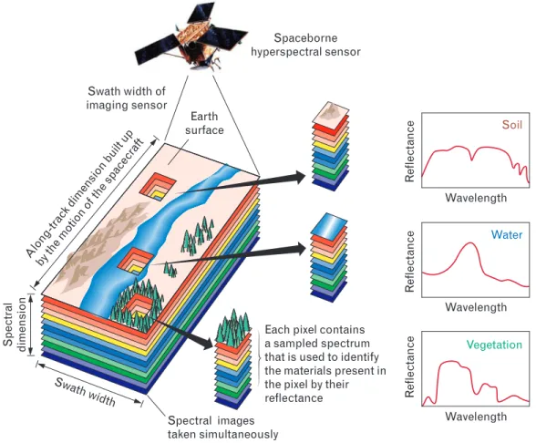
Throughout this special issue of the Journal we refer to the illumination conditions in a scene as well as the reflectance properties of materials and surfaces in that scene. Irradiance refers to the light energy per unit time (power) impinging on a surface, normalized by the surface area, and is typically specified in watts per square meter (W/m2). Reflectance is a unitless number between 0 and 1 that characterizes the fraction of in-cident light reflected by a surface. Reflectance may be further qualified by parameters such as the wave-length of reflected light, the angle of incidence, and the angle of reflection. Radiance is an important re-lated concept that does not distinguish between the light illuminating a surface or the light reflected from Spectral images taken simultaneously Wavelength Re fl e c tance Wavelength Wavelength Vegetation Water Soil
Each pixel contains a sampled spectrum that is used to identify the materials present in the pixel by their reflectance Swa th width Spe ctr al dimension Along-tr
ack dimension built up
by the motion o f the space craft Earth surface Spaceborne hyperspectral sensor Swath width of imaging sensor R efl e c ta n c e R efl e c ta n c e
FIGURE 1. The concept of imaging spectroscopy. An airborne or spaceborne imaging sensor
simul-taneously samples multiple spectral wavebands over a large area in a ground-based scene. After ap-propriate processing, each pixel in the resulting image contains a sampled spectral measurement of reflectance, which can be interpreted to identify the material present in the scene. The graphs in the figure illustrate the spectral variation in reflectance for soil, water, and vegetation. A visual represen-tation of the scene at varying wavelengths can be constructed from this spectral information.
a surface. Radiance is simply the irradiance normal-ized by the solid angle (in steradians) of the observa-tion or the direcobserva-tion of propagaobserva-tion of the light, and is typically measured in W/m2/steradian. Normaliz-ing the radiance by the wavelength of the light, which is typically specified in microns (µm), yields spectral
radiance, with units of W/m2/µm/steradian.
Reflectance Spectrum
We are accustomed to using color as one of the ways we distinguish and identify materials and objects. The color and reflectivity of an object are typically impor-tant indications of the material composition of the object, since different materials absorb and reflect the impinging light in a wavelength-dependent fashion. To a first order, the reflected light, or spectral radiance Ls( )λ , that we see or that a sensor records is the prod-uct of the impinging scene radiance Li( )λ and the material reflectance spectrum ρ λ( ), both of which vary as a function of wavelength λ:
Ls( )λ = ρ λ( ) ( ) .Li λ (1) If the illumination spectrum is known, then the ma-terial reflectance spectrum, or reflectivity, can in prin-ciple be recovered from the observed spectral radiance over those regions of the spectrum in which the
illu-mination is nonzero. Since the reflectance spectrum is independent of the illumination, the reflectance spec-trum provides the best opportunity to identify the materials in a scene by matching the scene reflectance spectra to a library of known spectra.
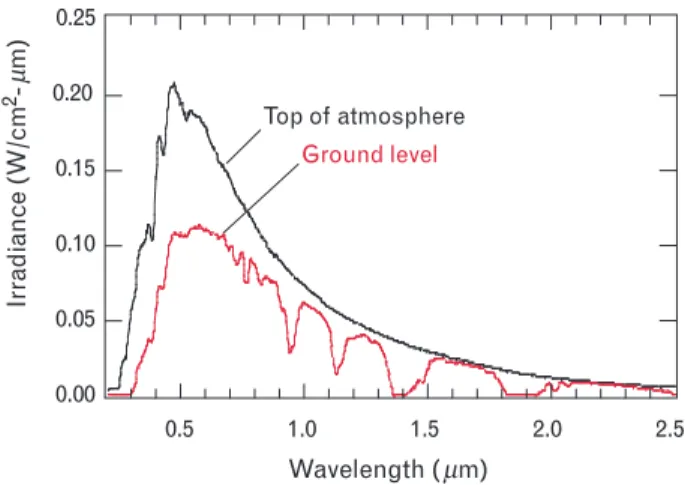
In the case of solar illumination, the spectral irradi-ance of the light reaching the atmosphere is reason-ably well characterized, as shown in Figure 2. Equa-tion 1, however, oversimplifies the relaEqua-tion between reflectance and illumination. Many environmental and sensing phenomena can complicate the recovery of the reflectance spectra. For example, even though the spectrum of the solar radiation reaching the atmo-sphere is well characterized, the spectrum of the solar radiation reaching the ground is altered in a tempo-rally and geographically dependent fashion because of propagation of solar radiation through the earth’s constantly changing atmosphere. Such atmospheric modulation effects must be accounted for in order to reliably recover the reflectance spectra of materials on the ground in a sunlit scene.
Sensor errors can further impede the recovery of reflectance spectra by distorting and contaminating the raw imagery. For example, focal-plane vibration can result in cross-contamination of adjacent spectral bands, thus distorting the observed spectrum. A com-prehensive discussion of sensor errors and artifacts is beyond the scope of this article. The next section, however, provides an overview of the image forma-tion process.
Image Formation and Area Coverage Rate
Collecting two-dimensional spatial images over many narrow wavebands with a two-dimensional focal-plane imaging sensor typically involves some form of time-sequenced imaging. This collection can be ac-complished by either a time sequence of two-dimen-sional spatial images at each waveband of interest, or a time sequence of spatial-spectral images (one-dimen-sional line images containing all the wavebands of interest), with multiple one-dimensional spatial im-ages collected over time to obtain the second spatial dimension.
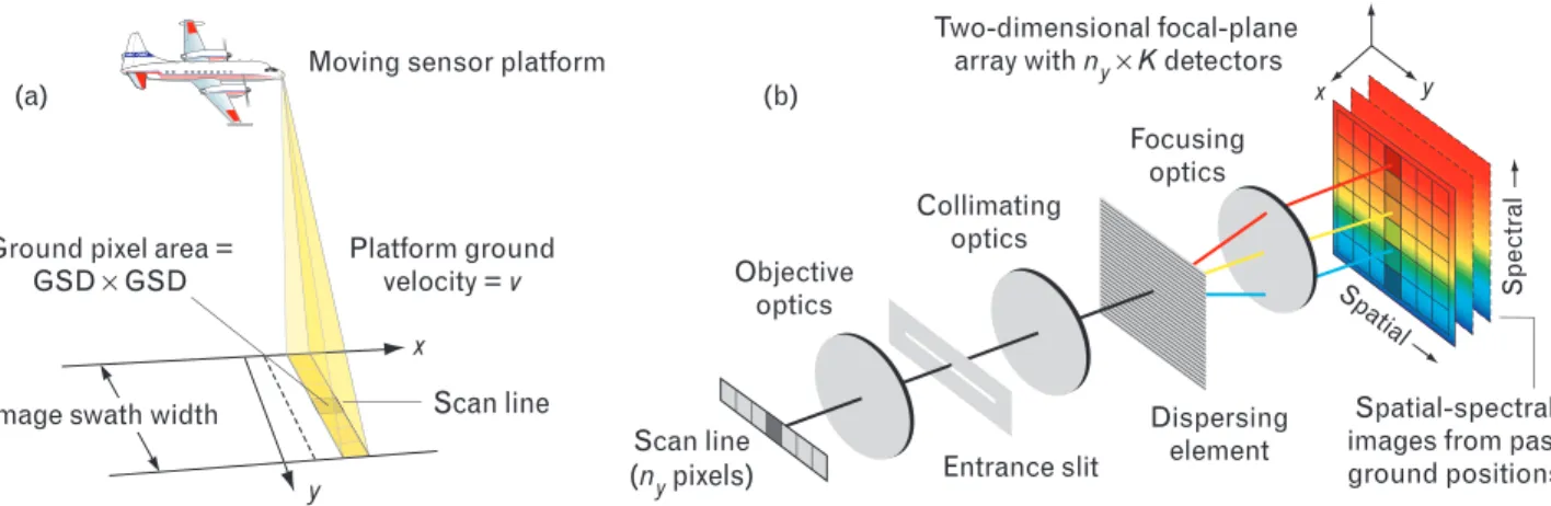
A variety of techniques have been developed to lect the required data. A common format for data col-lection is a push-broom imaging sensor, in which a
Irr adiance (W/cm 2µ- m) 0.20 0.15 0.10 0.05 0.00 0.5 1.0 1.5 2.0 2.5 Wavelength ( m)µ Top of atmosphere Ground level 0.25
FIGURE 2. Solar spectral irradiance curves at the top of the atmosphere and at ground level. The solar irradiance out-side the atmosphere (black curve) is well characterized. At ground level (red curve) it is altered by the absorption and scattering effects of the atmosphere. The recovery of reflec-tance spectra of different objects and materials must take into account the effects the atmosphere has on the spec-trum of both the solar illumination and the reflected light.
cross-track line of spatial pixels is decomposed into K spectral bands. Figure 3 illustrates the geometry for this type of data-collection system. The spectral de-composition can be accomplished by using any of several mechanisms, such as a diffraction grating or a wedge filter [1].
Historically, spectral imaging for remote sensing can be traced back to the Television Infrared Observa-tion Satellite (TIROS) series first launched in 1960 [2]. The TIROS legacy has continued with the Ad-vanced Very High Resolution Radiometer (AVHRR) and the Moderate Resolution Imaging Spectroradi-ometer (MODIS) instruments [3], launched aboard the Terra (Latin for earth) spacecraft in 1999. The spatial resolution of AVHRR is four kilometers, and the spatial resolution of the multispectral MODIS sensor varies from 250 meters in some spectral bands to one kilometer in others. In comparison, the focus of the articles in this issue of the Journal is on sensors with spatial resolutions better than thirty meters, and in some cases better than one meter.
Sampling
There are four sampling operations involved in the collection of spectral image data: spatial, spectral, ra-diometric, and temporal. In the systems discussed in this issue, we assume the spatial resolution is identical to the ground sample distance (GSD), although in general the GSD could be smaller than the spatial resolution. For the systems described in this issue, the
GSD varies from a fraction of a meter to tens of meters, and is established primarily by the sensor ap-erture and platform altitude. Platform altitude is loosely constrained by the class of sensor platform (e.g., spaceborne versus airborne).
As noted earlier, spectral sampling is achieved by decomposing the radiance received in each spatial pixel into a number of wavebands. The wavebands may vary in resolution, and may be overlapping, con-tiguous, or disparate, depending upon the design of the sensor. A color image, consisting of red, green, and blue bands, is a familiar example of a spectral sampling in which the wavebands (spectral channels) are non-overlapping and relatively broad.
An analog-to-digital converter samples the radi-ance measured in each spectral channel, producing digital data at a prescribed radiometric resolution. The result is a three-dimensional spectral data cube, represented by the illustration in Figure 4. Figure 4(a) shows the spectra in cross-track scan lines being gath-ered by an airborne sensor. Figure 4(b) shows the scan lines being stacked to form a three-dimensional hyperspectral data cube with spatial information in the x and y dimensions and spectral information in the z dimension. In Figure 4(b) the reflectance spectra of the pixels comprising the top and right edge of the image are projected into the z dimension and color coded according to the amplitude of the spectra, with blue denoting the lowest-amplitude reflectance values and red denoting the highest values.
FIGURE 3. (a) Geometry of a push-broom hyperspectral imaging system. The area coverage rate is the swath width times the
platform ground velocity v. The area of a pixel on the ground is the square of the ground sample distance (GSD). (b) An imag-ing spectrometer on the aircraft disperses light onto a two-dimensional array of detectors, with ny elements in the cross-track (spatial) dimension and K elements in the spectral dimension, for a total of N = K × ny detectors.
Spa tial
Scan line
Moving sensor platform
Scan line (nypixels) Platform ground velocity = v Objective optics Entrance slit Collimating optics Dispersing element Focusing optics Two-dimensional focal-plane
array with ny× K detectors
x z
y
Ground pixel area = GSD × GSD
Spatial-spectral images from past ground positions
Spe
ctr
al
Image swath width
x
y
Spatial dimensions Tree Fabric Paint Grass 100–0–200 spectral channels Grass Grass Roads Man-made objects T T Tr T T T ereree T T T ee T T Moving sensor platform
Scan line (1× ny pixels) esss ees e e e e R efl e c ta nce
Water-vapor absorption bands Grass Tree Fabric Paint P P 0.4 mµ Wavelength( )λ 2.5 mµ Three-dimensional hypercube is assembled by stacking two-dimensional spatial-spectral scan lines (a) (b) (c) (d) Successive scan lines Spatial pixels Spectral channels x y z y x
FIGURE 4. Structure of the hyperspectral data cube. (a) A push-broom sensor on an airborne or spaceborne platform collects
spectral information for a one-dimensional row of cross-track pixels, called a scan line. (b) Successive scan lines comprised of the spectra for each row of cross-track pixels are stacked to obtain a three-dimensional hyperspectral data cube. In this illustra-tion the spatial informaillustra-tion of a scene is represented by the x and y dimensions of the cube, while the amplitude spectra of the pixels are projected into the z dimension. (c) The assembled three-dimensional hyperspectral data cube can be treated as a stack of two-dimensional spatial images, each corresponding to a particular narrow waveband. A hyperspectral data cube typi-cally consists of hundreds of such stacked images. (d) Alternately, the spectral samples can be plotted for each pixel or for each class of material in the hyperspectral image. Distinguishing features in the spectra provide the primary mechanism for de-tection and classification of materials in a scene.
Secondary illumination Atmospheric absorption and scattering Upwelling radiance Spatial resolution and viewing angle
of the sensor Illumination angle
of the sun
Image pixel projection
FIGURE 5. Atmospheric and scene-related factors that can
contribute to degradations in the imaging process. The spa-tial resolution of the sensor and the degree of atmospheric scattering and absorption are the most significant contribu-tors to diminished image quality.
The spectral information in the z dimension might be sampled regularly or irregularly, depending on the design of the sensor. Spectral image data can be viewed as a stack of two-dimensional spatial images, one image for each of the sampled wavebands, as shown in Figure 4(c), or the image data can be viewed as individual spectra for given pixels of interest, as shown in Figure 4(d). (Note: In Figure 4, color in parts c and d represents spectral bands rather than re-flectance amplitudes.)
While there is an integration time τd associated with the image formation process, we use the term
temporal sampling to refer not to the time associated
with image formation, but to the process of collecting multiple spectral images of the same scene separated in time. Temporal sampling is an important mecha-nism for studying natural and anthropogenic changes in a scene [4, 5].
Practical Considerations
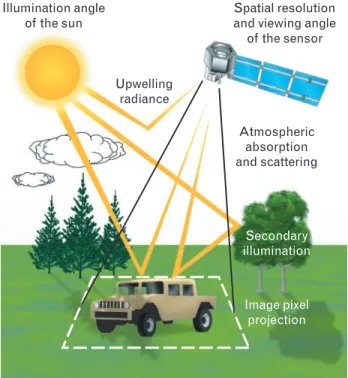
The concept of spectral imaging, as illustrated in Fig-ure 1, appears straightforward. There are many prac-tical issues, however, that must be addressed in the design and implementation of a spectral imaging sys-tem. These issues include the spatial and spectral reso-lution of the sensor, atmospheric effects such as ab-sorption and scattering, the spectral variability of surface materials in the scene, and other environmen-tal effects such as viewing angle, secondary illumina-tion, and shadowing. Figure 5 illustrates a number of these salient issues for a representative scene.
Spatial Resolution
Sensor cost is usually a strong function of aperture size, particularly for spaceborne systems. Reducing the aperture size reduces sensor cost but results in de-graded spatial resolution (i.e., a larger GSD). For a spectral imager, the best detection performance is ex-pected when the angular resolution of the sensor, specified in terms of the GSD, is commensurate with the footprint of the targets of interest. Targets, how-ever, come in many sizes. Consequently, for a given sensor design, some targets may be fully resolved spa-tially, while others may fill only a fraction of the GSD footprint that defines a pixel. Therefore, detection and identification algorithms must be designed to
function well regardless of whether targets are fully re-solved (i.e., fully fill a pixel) or comprise only a frac-tion of the material in a given pixel (i.e., subpixel).
Atmospheric Effects
The atmosphere absorbs and scatters light in a wave-length-dependent fashion. This absorption and scat-tering has several important implications that cause difficulties for sensor imaging. Four of these difficul-ties are described below.
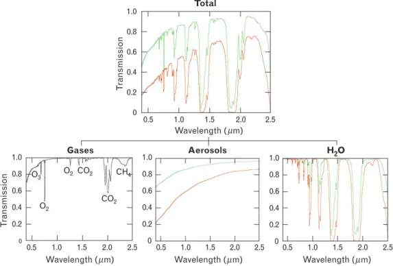
First, the atmosphere modulates the spectrum of the solar illumination before it reaches the ground, and this modulation must be known or measured in order to separate the spectrum of the illumination (the impinging solar radiance) from the reflectivity (the reflectance spectrum) that characterizes the materials of interest in the scene. Figure 6 shows the one-way total atmospheric transmission curve for two different water vapor and aerosol conditions, corre-sponding to extremes of wet and dirty versus clean and dry atmospheres. Figure 6 also shows the
contri-butions of well-mixed gases, aerosols, and water vapor to the overall transmission. As the solar-illumination angle and the viewing angle of the sensor change, the total path through the atmosphere changes, which in turn affects the total atmospheric transmission. Also, the water-vapor distribution (as well as the aerosol characteristics of the atmosphere) varies with location and time, so the methods of compensating for these effects must be scene based.
Second, some of the solar radiation is scattered by the atmosphere into the field of view of the sensor without ever reaching the ground. This scattered light is superimposed on the reflected light arriving from the scene, and is termed path radiance because it ap-pears along the line-of-sight path to the scene. Third, the solar radiation scattered by the atmosphere, pre-dominantly in the blue region of the visible spectrum, acts as a secondary source of diffuse colored illumina-tion. This diffuse sky illumination is most important for shadowed objects, since regions shadowed from the direct rays of the sun may still be illuminated by the diffuse non-white sky radiation. Fourth, the solar
illumination that reaches the scene and is reflected by the target is further absorbed and scattered by the at-mosphere as it propagates toward the sensor.
A number of methods are currently used to esti-mate and compensate for these atmosphere propaga-tion effects. The appendix entitled “Fundamentals of Atmospheric Compensation” provides additional de-tail on these compensation methods.
Other Environmental Effects
In addition to atmospheric absorption and scattering, several other prominent environmental parameters and associated phenomena have an influence on spec-tral imaging. The sun angle relative to zenith, the sen-sor viewing angle, and the surface orientation of the target all affect the amount of light reflected into the sensor field of view. Clouds and ground cover may cast shadows on the target, substantially changing the illumination of the surface. Nearby objects may also reflect or scatter sunlight onto the target, superimpos-ing various colored illuminations upon the dominant direct solar illumination, as illustrated in Figure 5.
FIGURE 6. Effect of atmospheric gases, aerosols, and water vapor on total atmospheric transmission.
The green curves represent the case of modest influence (0.4 cm col of water vapor), which corresponds to a rural environment with a visual range of 23 km. The red curves represent the case of strong influence (4.1 cm col of water vapor), which corresponds to an urban environment with a visual range of 5 km.
Total 0.5 1.0 1.5 2.0 2.5 0.8 0.6 0.4 0.2 0 1.0 Gases CO2 CO2 O2 O2 O3 CH4 0.5 1.0 1.5 2.0 2.5 0.8 0.6 0.4 0.2 0 1.0 Aerosols 0.5 1.0 1.5 2.0 2.5 0.8 0.6 0.4 0.2 0 1.0 H2O 0.5 1.0 1.5 2.0 2.5 0.8 0.6 0.4 0.2 0 1.0
Wavelength ( m) Wavelength ( m) Wavelength ( m) Wavelength ( m) Tr ansmission Tr ansmission µ µ µ µ
0.4 0.6 0.8 1 1.2 1.4 1.6 1.8 2 2.2 2.4 0 0.1 0.2 0.3 0.4 0.5 Full pixels (114) Wavelength ( m) µ Reflectance Mean spectrum
FIGURE 7. Example of variability in reflectance spectra measured over multiple instances of a given material (in this case, vehicle paint) in a scene. The shapes of the spectra are fairly consistent, but the amplitudes vary con-siderably over the scene. To exploit this spectral shape invariance, some detection algorithms give more weight to the spectral shape than to the spectral amplitude in determining whether a given material is present in a pixel. The gaps correspond to water-vapor absorption bands where the data are unreliable and are discarded.
Spectral Variability
Early in the development of spectral imaging, re-searchers hypothesized that the reflectance spectrum of every material is unique and, therefore, represents a means for uniquely identifying materials. The term “spectral signature,” which is still in use today, sug-gests a unique correspondence between a material and its reflectance spectrum. In field data, however, as well as laboratory data, we observe variability in the reflectance spectrum of most materials. Many mecha-nisms may be responsible for the observed variability, including uncompensated errors in the sensor, un-compensated atmospheric and environmental effects, surface contaminants, variation in the material such as age-induced color fading due to oxidation or bleaching, and adjacency effects in which reflections from nearby objects in the scene change the apparent illumination of the material. Seasonal variations also introduce enormous changes in the spectral character of a scene. We need only observe the changes in a de-ciduous forest over spring, summer, fall, and winter to appreciate the degree of spectral variability that can arise in the natural materials comprising a scene.
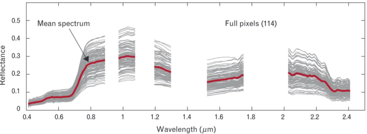
There is some reason to expect that man-made ma-terials exhibit less spectral variability than the natu-rally occurring materials in a scene. Figure 7 shows a number of instances of reflectance spectra derived for multiple occurrences of fully resolved vehicle-paint
pixels in a scene. Note that while the shapes of the spectra are fairly consistent, the amplitude varies con-siderably over the scene. In an effort to exploit the spectral shape invariance, some of the more successful detection algorithms give more weight to the spectral shape than to the amplitude when determining whether a particular material is present in a pixel.
Motion and Sensor Artifacts
As indicated in Figure 3, spectral imaging sensors typically exploit sensor platform motion as a means of scanning a scene. However, nonlinear motion of the sensor can corrupt the spectral image by mixing to-gether the spectral returns from different parts of the spatial image. Motion of objects in the scene can also create artifacts if the motion is on the order of the GSD during the integration time τd. This type of spa-tial migration can degrade image quality, but fortu-nately it is not as significant as the spectral migration in terms of impact on subsequent processing for de-tection and identification of materials. The imaging of a scene, including detection and conversion of the radiance to a digital sequence, introduces a number of artifacts such as thermal noise, quantization, and geo-metric distortion. The nature of these sensor artifacts, and methods for modeling them, are discussed in more detail in the article entitled “Hyperspectral Im-aging System Modeling,” by John P. Kerekes and Jerrold E. Baum.
Spatial versus Spectral Information
The emergence of radar sensors in the late 1930s opened the door to detection and discrimination of radar-reflecting targets without relying on traditional spatial imagery. Less than sixteen years after the intro-duction of the first operational radar, however, re-searchers were flying experimental side-looking air-borne radars (SLAR) in order to transform radar returns into images [6]. Synthetic aperture radar (SAR) was devised to create images from two-dimen-sional range-Doppler radar reflectance maps [7]. In-terferometric SAR was developed later as a means of generating three-dimensional radar images [8]. The introduction of light detection and ranging (lidar) technology provided another way to create three-di-mensional images in the form of high-resolution angle-angle-range reflectance maps. Throughout the evolution of passive and active imaging methods, im-proved spatial resolution has been a mantra of devel-opment that has pushed optical sensors to larger aper-tures and radar sensors to higher frequencies. Automated detection and recognition algorithms have evolved along with these sensors, but human vi-sual analysis continues to be the predominant means of interpreting the imagery from operational imaging sensors.
Multispectral Imaging
Increasing the spatial resolution of imaging sensors is an expensive proposition, both in terms of the sensor and in terms of the amount of sensor data that must subsequently be processed and interpreted. The trained human analyst has traditionally carried the main burden of effective image interpretation, but as technology continues to advance, the volume of high-resolution optical and radar imagery has grown at a faster rate than the number of trained analysts.
In the 1960s, the remote sensing community, rec-ognizing the staggering cost of putting large passive imaging apertures in space, embraced the concept of exploiting spectral rather than spatial features to iden-tify and classify land cover. This concept relies prima-rily on spectral signature rather than spatial shape to detect and discriminate among different materials in a scene. Experiments with line-scanning sensors
pro-viding up to twenty spectral bands in the visible and infrared were undertaken to prove the concepts [9]. This experimental work helped create interest and support for the deployment of the first space-based multispectral imager, Landsat-1 [10], which was launched in 1972 (Landsat-1 was originally desig-nated the Earth Resource Technology Satellite, or ERTS 1). Landsat-7, the latest in this series of highly successful satellites, was launched in 1999. A Lincoln Laboratory prototype for a multispectral Advanced Land Imager (ALI) was launched in November 2000 aboard the National Aeronautics and Space Adminis-tration (NASA) Earth Observing (EO-1) satellite [11]. EO-1 also carries a VNIR/SWIR hyperspectral sensor, called Hyperion, with 220 spectral bands and a GSD of thirty meters.
Hyperspectral Imaging
On the basis of the success of multispectral sensing, and enabled by advances in focal-plane technology, researchers developed hyperspectral sensors to sample the expanded reflective portion of the electromag-netic spectrum, which extends from the visible region (0.4 to 0.7 µm) through the SWIR (about 2.5 µm) in hundreds of narrow contiguous bands about ten na-nometers wide. The majority of hyperspectral sensors operate over the VNIR/SWIR bands, exploiting solar illumination to detect and identify materials on the basis of their reflectance spectra.
If we consider the product of spatial pixels times spectral bands (essentially the number of three-di-mensional resolution cells in a hypercube) to be a measure of sensor complexity, then we can preserve the overall complexity in going from a panchromatic sensor (with one broad spectral band) to a hyperspec-tral sensor (with several hundred narrow spechyperspec-tral bands) by reducing the number of spatial pixels by a factor of several hundred while keeping the field of view constant. In effect, a one-dimensional reduction in spatial resolution by a factor of approximately fif-teen (i.e., the square root of K, the number of spectral bands, which is typically about 220) compensates for the increased number of spectral samples and reduces the required aperture diameter by the same factor, thus reducing the potential cost of a sensor. However, while the total number of three-dimensional
resolu-tion cells is preserved, the informaresolu-tion content of the image is generally not preserved when making such trades in spatial versus spectral resolution.
Area Coverage Rate
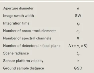
In many cases, a primary motivation for applying spectral imaging to remote sensing is to reduce the re-quired spatial resolution—and thus the size and weight—of the sensor. Therefore, it is worthwhile, even in this brief overview, to consider the design trade-offs involved in selecting the spatial and spectral resolution of a spectral imaging sensor. Table 1 sum-marizes the important spectral image formation pa-rameters in this discussion.
When the achievable signal-to-noise ratio (SNR) is limited by the imaging process in the sensor and not by noise (interference) in the scene, the SNR2 of the sensor grows in proportion to the product of the re-ceive aperture area d2, the area of a pixel on the ground (which for the purpose of this simple analysis we equate to the square of the GSD), the time inter-val τd over which the signal is integrated at the detec-tor, and the scene radiance Ls at the sensor:
SNR2 ∝ d2 ×GSD2 ×τd ×Ls. (2) The integration time is proportional to the GSD di-vided by the platform velocity v :
τd v ∝ GSD.
In a spectral imaging sensor, the radiance signal from each pixel is decomposed into K spectral bands, so that the average spectral radiance Lλ in each spectral band (detector) on the focal plane is
L L
K s λ ∝ .
Substituting for τd in Equation 2, and absorbing the scene-radiance scale factor into the proportionality sign, the SNR proportionality at the detector can be expressed as SNR2 GSD 2 3 ∝ × × d v K . (3)
To relate this expression to area coverage rate (ACR), we note from Figure 3 that the swath width (SW) is
equal to the GSD times the number of cross-track samples:
SW = GSD×( / ) ,N K
where N is the total number of detectors in the focal plane. Therefore, Equation 3 can be rewritten as
SNR GSD SW 2 2 4 2 ∝ × × × × d N v K .
The achievable ACR is then given by
ACR SW GSD SNR ≡ × ∝ × × × v d N K 2 4 2 2 .
By fixing the aperture size d and the number of detec-tors N on the focal plane, we find that the ACR is proportional to the square of the ground sample area, and inversely proportional to both the square of the SNR and the square of the number of spectral bands:
ACR GSD SNR ∝ × 4 2 K2. (4)
Spatial versus Spectral Trade-Space Example
The expression for ACR given in Equation 4 can be evaluated to further quantify the trade-off between spectral and spatial resolution. Consider, as a baseline for comparison, a panchromatic imaging system (K = 1), with GSD = 0.3 m, SNR = 100, and ACR = 30 km2/hr. In the following comparison we consider
Table 1. Spectral Image Formation Parameters
Aperture diameter d
Image swath width SW
Integration time τd
Number of cross-track elements ny Number of spectral channels K
Number of detectors in focal plane N (= ny× K)
Scene radiance Ls
Sensor platform velocity v
a 10-band system to be representative of a multispec-tral sensor, and a 100-band system to be representa-tive of a hyperspectral system.
According to Equation 4, increasing the number of spectral bands while maintaining the GSD and detec-tor SNR constant results in a decrease in ACR. Since a primary rationale for multispectral and hyperspec-tral imaging is to reduce reliance on high spatial reso-lution for detection and identification, the ACR can be preserved while increasing the number of spectral bands by increasing the GSD (i.e., reducing the spa-tial resolution). According to Equation 4, one way to preserve the ACR when increasing the spectral bands by K is to reduce the GSD by a factor of K1/2. How-ever, since each pixel is decomposed into K bands, detection processing such as matched filtering, which
combines the K bands for detection, can yield an im-provement in SNR of K1/2, which is the gain from noncoherent integration of K samples. Therefore, it makes sense to reduce the SNR in each detector by
K1/2 and increase the GSD by a smaller amount. An increase in GSD by K1/4 and a decrease in SNR by
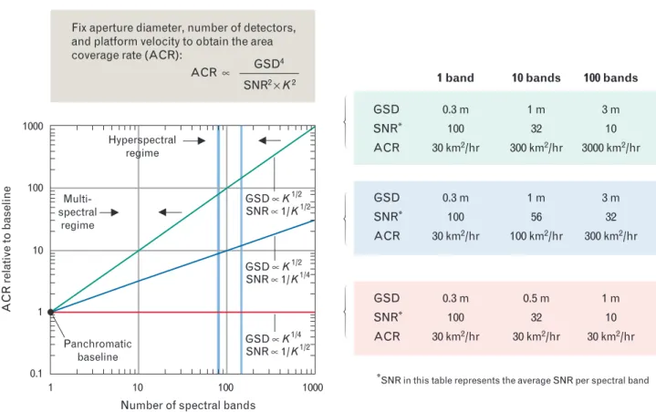
K1/2 preserves the overall ACR. A decrease in the pixel SNR by K1/2 along with an increase in GSD by K1/2 increases the ACR by a factor of K, relative to the baseline panchromatic sensor. Figure 8 shows these spectral-versus-spatial trades and the impact on ACR. In Figure 8 the performance of the baseline pan-chromatic sensor (one spectral band) is represented by the convergence of the three curves at the normal-ized ACR of 1.0. As more spectral bands are added, the ACR can be preserved by letting the GSD grow in
0.1 1 10 100 1000 10 1 100 1000
Number of spectral bands Fix aperture diameter, number of detectors, and platform velocity to obtain the area coverage rate (ACR):
GSD SNR* ACR GSD SNR* ACR GSD SNR* ACR 10 bands 1 m 32 300 km2/hr 1 m 56 100 km2/hr 0.5 m 32 30 km2/hr 100 bands 3 m 10 3000 km2/hr 3 m 32 300 km2/hr 1 m 10 30 km2/hr GSD ∝ K1/2 SNR ∝ 1/ K1/2 GSD ∝ K1/2 SNR ∝ 1/ K1/4 GSD ∝ K1/4 SNR ∝ 1/ K1/2 Hyperspectral regime GSD4 SNR2 × K2 Multi- spectral regime ACR ∝ Panchromatic baseline
ACR relative to baseline
1 band 0.3 m 100 30 km2/hr 0.3 m 100 30 km2/hr 0.3 m 100 30 km2/hr
*SNR in this table represents the average SNR per spectral band
FIGURE 8. Example of trade space for spatial, spectral, and area coverage rate (ACR). The plot on the left shows the
improve-ment in ACR that can be achieved with a multiband spectral sensor by trading spatial resolution for spectral resolution. The baseline reference system is a single-band panchromatic imager with a resolution of 0.3 m and an ACR of 30 km2/hr. The red curve represents the family of multiband imagers that achieve the same ACR as the baseline by simultaneously reducing the spatial resolution (i.e., increasing GSD) and the SNR in an individual detector. The GSD and SNR for a single-band panchro-matic system, a 10-band multispectral system, and a 100-band hyperspectral system are shown in the red box in the table to the right. The blue and green curves correspond to other trades in which the ACR of the multiband sensor is increased relative to the panchromatic baseline. The table again provides specific values of GSD, SNR, and ACR for the case of a 10-band multi-spectral system and a 100-band hypermulti-spectral system.
proportion to K1/4 while the detector SNR is allowed to decrease in proportion to 1/K1/2, as represented by the red curve. The companion table shows examples of the resulting GSD and SNR for the cases when
K = 10 and K = 100, corresponding to representative
multispectral and hyperspectral sensors. The blue curve represents a design trade in which the ACR is increased by a factor of K1/2 over the panchromatic baseline. Note from the table that the factor of K1/2 = 10 improvement in ACR for K = 100 is achieved at the cost of an SNR reduction per detector of K1/4 = 3.2. Matched filtering of the spectral information in a pixel may compensate for much of the reduction in SNR within the individual detectors.
High-Dimensional Data Representation
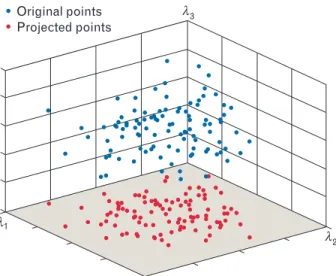
The manner in which spectral image data are pro-cessed is strongly influenced by the high dimensional-ity of the data. To illustrate the concept of data di-mensionality, we consider a multispectral image
sensor with only three wavebands, λ1, λ2, and λ3. As in the high-dimensional case, the wavelength-depen-dent reflectivity of a material is used to characterize the material. For this low-dimensional example, if a number of different materials are measured, each ma-terial can be represented as a data point in a three-di-mensional space, as indicated by the blue dots in Fig-ure 9. Each unique point in this space represents a spectral signature defined by the 3-tuple (λ1, λ2, λ3). The spectral signature is thus seen as a vector of length—or dimension—three. This representation is highly compatible with many numerical processing algorithms.
Dimensionality Reduction
Depending upon the nature of the data, it may be possible to project the data cloud into a lower dimen-sional space while still preserving the separation and uniqueness of the data points. Figure 9 illustrates this process, in which the three-dimensional representa-tion (indicated by blue dots) is projected onto a two-dimensional plane (indicated by red dots), thus re-ducing the dimensionality by one. If two or more of the blue dots project onto the same point in the two-dimensional plane, it is no longer possible to distin-guish the projected blue points as unique. In general, finding a projection that preserves the relevant infor-mation content of the data (separation) while reduc-ing dimensionality is a complicated undertakreduc-ing. The article in this issue by Nirmal Keshava entitled “A Survey of Spectral Unmixing Algorithms” describes this topic in greater detail.
The same concept of dimensionality illustrated in Figure 9 can be applied to hyperspectral sensors with hundreds of contiguous spectral wavebands. Unlike the three-dimensional example, all the information contained in a high-dimensional data cloud cannot be visualized by a two-dimensional or three-dimen-sional perspective plot. At best, we can construct two-dimensional and three-two-dimensional visualizations by projecting the K-dimensional spectral vector into an appropriately chosen two-dimensional or three-di-mensional subspace.
An important implication of the dimension-reduc-tion example is that, unlike convendimension-reduc-tional panchro-matic and color imagery, higher-dimension hyper-λ1
Original points Projected points
λ2
λ3
FIGURE 9. Example of data from a multispectral image
sen-sor with only three wavebands, λ1, λ2, and λ3. In this
three-dimensional example, the wavelength-dependent reflectivity of a material is measured in each of the three wavebands and used to characterize the material. If a number of differ-ent materials are measured, each material can be repre-sented as a data point in a three-dimensional space, as indi-cated by the blue dots. Dimensionality reduction of the data is illustrated by projecting the data cloud into a lower dimen-sional space defined by the (λ1, λ2) plane. The projected
data, represented by red dots, still preserve the uniqueness of the original data points, although the separation in Eu-clidean distance between the data points is reduced.
spectral imagery requires computer processing for maximum information extraction and visualization. This processing can be totally automated or it can be accomplished with guidance from an image analyst. After processing is completed, the information can be highlighted, perhaps with pseudocolor, and displayed in a two-dimensional image, but the computer-pro-cessing step is an essential precursor to visualization.
How Many Dimensions Are Needed?
If the task is to discriminate between a particular tar-get material and a particular class of background, a few well-chosen wavebands are usually sufficient to separate the target and background materials. If this is true, we might well question the motivation for hy-perspectral sensing, in which hundreds of contiguous narrow wavebands are measured by the sensor. Differ-ent materials, however, exhibit differDiffer-ent spectral fea-tures. Certain paints and vegetation can be character-ized by broad, slowly varying spectral features. Other materials, such as minerals and gases, possess very narrow spectral features, and the location of these narrow features in the spectral band differs for each class of material. Therefore, narrow wavebands may be needed to resolve features that help differentiate similar spectra, and contiguous bands are needed to handle the expected variety of materials, since impor-tant features may be in different spectral locations for each material. In addition, the narrow wavebands that straddle the water-vapor absorption bands are important in estimating and correcting for the vari-able water vapor contained in the atmosphere.
Thus, if we were interested in only a few target ma-terials and backgrounds, a limited number of cafully chosen narrow wavebands would suffice to re-cover the salient spectral features. As more types of targets and backgrounds are added to the list, how-ever, the number and location of wavebands needed to discriminate between any given spectral pair grows rapidly. One possible solution would be to build many special-purpose sensors, each of which collects only a minimal set of wavebands needed for a limited set of targets and backgrounds. A more cost-effective and robust solution is to build one type of sensor that oversamples the spectral information, and to develop application-specific algorithms, or a family of
algo-rithms, that remove the redundant or undesired spec-tral information while preserving the information relevant to a given application. The essence of hyper-spectral processing for detection and identification of materials is the extraction of salient features and the suppression of redundant or common features. Spectral Imaging Applications
By oversampling the spectral information, we can ap-ply hyperspectral imaging sensors to a variety of dis-tinctly different problems, adapting the processing used to extract relevant information. There is much value, however, in tailoring the spatial resolution and sensor field of view for the intended class of applica-tion. Higher spatial resolution provides an improved signal-to-background-interference ratio for spatially small targets, usually at the cost of decreased sensor field of view. In general, the spatial resolution of the sensor is chosen on the basis of the spatial extent of the primary targets of interest. Figure 10 presents a simplified taxonomy of the many different types of hyperspectral imaging applications, identifying three major categories: anomaly detection, target recogni-tion, and background characterization.
Anomaly Detection
Anomaly detection is characterized by the desire to locate and identify uncommon features in an image. These features could be man-made materials dis-persed in a natural background, or they could be de-partures of the natural features from the norm. One of the early applications of multispectral imaging was to detect the spread of corn blight in the Midwest [10]. This application depends primarily on being able to distinguish brown withered leaves interspersed in fields of healthy green corn stalks.
Target Recognition
Target recognition is distinguished from anomaly de-tection by the availability of some a priori informa-tion about the target. This informainforma-tion could be a li-brary of spectral reflectance signatures associated with targets, or less explicit information such as a reflec-tance signature extracted from within the scene. For example, anomaly detection could be used to isolate specific materials in a scene, and subsequent passes of
an imaging sensor might be used to search for similar materials as well as to verify that the previously de-tected objects or materials have not moved. With a spectral library, materials might be identified and as-sociated with specific types of targets, thus providing a form of target recognition.
Background Characterization
The first two application categories listed in Figure 10 emphasize detection and identification of spatially isolated features in an image, in the form of anomalies or targets. The third category emphasizes overall background scene analysis and identification, and spans the domains of land, ocean, and atmosphere. Because the Landsat imaging program has operated for over thirty years, much of the spectral image data collected to date has been oriented toward land char-acterization, employing multispectral sensors with GSD values of thirty meters or more.
An example of background scene characterization is coastal characterization, including shallow-water bathymetry. The sidebar entitled “Hyperspectral ver-sus Multispectral Remote Sensing for Coastal Char-acterization” illustrates the evolution of multispectral sensors for this application and shows examples of the information products that can be derived from multi-spectral and hypermulti-spectral data.
Spectral Processing
As implied in the previous section, the number and variety of applications for hyperspectral remote sens-ing are potentially quite large. However, the majority of algorithms used in these applications can be orga-nized according to the following primitive applica-tion-specific tasks: (a) searching the pixels of a hyper-spectral data cube for rare hyper-spectral signatures (anomaly detection or target detection); (b) finding the significant (i.e., important to the user) changes be-tween two hyperspectral scenes of the same geo-graphic region (change detection); (c) assigning a label or class to each pixel of a hyperspectral data cube (classification); and (d) estimating the fraction of the pixel area occupied by each material present in the pixel (unmixing). Note that from a signal processing perspective, task c (labeling pixels) is a classification problem, whereas task d (determining the constituent elements of a pixel) is an estimation problem.
Preliminary Processing to Reduce Dimensionality
Raw data from the sensor must usually undergo a se-ries of calibration and correction operations to com-pensate for artifacts and gain variations in the sensor. The result is a calibrated radiance cube, which may be processed directly, or it may have atmospheric
com-Target recognition Anomaly detection Cueing Change detection Status monitoring Recognition Land surface Background characterization Ocean Atmosphere Detection Natural features Man-made objects
Hyperspectral Imaging Applications
Classification Material identification Status characterization Terrain categorization Trafficability Target characterization Coastal bathymetry Water clarity Underwater hazards Water vapor and aerosols Cloud/plume differentiation Atmospheric compensation Stressed vegetation Wet ground Natural effluents Potential targets Search and rescue Man-made effluents
FIGURE 10. Simplified taxonomy of applications for hyperspectral imaging. The three major application categories are anomaly
detection, target recognition, and background characterization. Anomaly detection divides pixels into man-made objects or natural features, target recognition provides detection parameters along with classification parameters of potential targets, and background characterization identifies the condition of natural features associated with land, ocean, or atmosphere.
pensation applied to it to produce a reflectance cube. Once a calibrated data cube is produced, dimension-ality reduction of the data prior to application of de-tection or classification algorithms can lead to signifi-cant reductions in overall computational complexity. Reducing data dimensionality also reduces the num-ber of pixels required to obtain accurate estimates of statistical parameters, since the number of samples (pixels) required to obtain a statistical estimate with a given accuracy is generally proportional to some power of the data dimensionality. The most widely used algorithm for dimensionality reduction is princi-pal-component analysis (PCA), which is the discrete analog to the Karhunen-Loève transformation for continuous signals. The PCA algorithm is described in more detail in the article in this issue entitled “En-hancing Hyperspectral Imaging System Performance with Sensor Fusion,” by Su May Hsu and Hsiao-hua K. Burke.
Figure 11 is a simplified block diagram of the spec-tral processing chain, starting with a calibrated radi-ance cube, and illustrating the common elements of atmospheric compensation and dimensionality re-duction. Subsequent specialized processing depends on the intended application. Figure 11 illustrates two
of many possible applications, unmixing and
detec-tion, each of which is discussed briefly in the
follow-ing sections and developed more fully in companion articles in this issue.
Classification versus Detection
Formally, classification is the process of assigning a la-bel to an observation (usually a vector of numerical values), whereas detection is the process of identifying the existence or occurrence of a condition. In this sense, detection can be considered as a two-class clas-sification problem: target exists or target does not ex-ist. Traditional classifiers assign one and only one la-bel to each pixel, producing what is known as a thematic map. This process is called hard
classifica-tion. The need to deal more effectively with pixels
containing a mixture of different materials, however, leads to the concept of soft classification of pixels. A soft classifier can assign to each pixel multiple labels, with each label accompanied by a number that can be interpreted as the likelihood of that label being cor-rect or, more generally, as the proportion of the mate-rial within the pixel.
In terms of data products, the goal of target-detec-tion algorithms is to generate target maps at a
con-Reflectance Radiance Atmospheric compensation Data/dimension reduction End-user applications j < K bands N pixels K bands Detection Unmixing
FIGURE 11. Simplified spectral processing diagram. The spectral processing typically starts with
calibra-tion of the data cube, followed by atmospheric compensacalibra-tion and dimensionality reduccalibra-tion. Subsequent specialized processing is determined by the intended end-user application, such as unmixing or detection.
FIGURE A. Spaceborne multispectral ocean sensors from 1976 to the present, showing the numbers and locations of spectral bands. The variety of bands indicates the ocean characteristics the sensors are designed to investigate. (Figure courtesy of the International Ocean Colour Coordinating Group, taken from IOCCG Report no. 1, 1998.)
H Y P E R S P E C T R A L V E R S U S M U L T I S P E C T R A L
R E M O T E S E N S I N G F O R C O A S T A L
C H A R A C T E R I Z A T I O N
350 400 450 500 550 600 650 700 750 800 850 900 950 CZCS OCTS POLDER MOS SeaW iFS MODIS MERIS 443 520550 670 750 412 443 490 520 565 670 765 865 443 490 565 670 763 765 865 910 408 443 485 520 570 615 650 685 750 815 870 412 443 490 510 555 670 765 865 412 443 488 531551 667678 748 870 870 779 709 681 665 620 560 510 490 442.5 412.5 412 443 490 510 555 670 765 865 443 510 555 670 865 443 490510 555 670 865 490 380 412 400 443 460 490 520 545 565 625 666 710 749 865 443 490 565 670 763765 865 910 OCM OCI OSMI GLI POLDER-2 S-GLI 350 400 450 500 550 600 650 700 750 800 850 900 950 (nm) MISR 867 672 557 446 680 412 443 490 520 565 625 680 710 749 865 λ two-thirds ofthe earth’s surface. The optical properties of ocean water are in-fluenced by many factors, such as phytoplankton, suspended mate-rial, and organic substances. Spectral remote sensing provides a means of routinely monitoring this part of our planet, and ob-taining information on the status of the ocean.
Ocean waters are generally partitioned into open ocean and coastal waters. Phytoplankton is the principal agent responsible for variations in the optical prop-erties of open ocean. Coastal wa-ters, on the other hand, are influ-enced not just by phytoplankton and related particles, but also by other substances, most notably inorganic particles in suspension and organic dissolved materials. Coastal characterization is thus a far more complex problem for optical remote sensing.
Figure A illustrates a variety of multispectral ocean color sensors used in the past twenty-five years. The spectral bands of these sen-sors, which lie in the spectral range between 0.4 and 1.0 µm, were chosen to exploit the reflec-tion, backscatter, absorpreflec-tion, and fluorescence effects of various ocean constituents. These multi-spectral sensors vary in the num-ber of bands and exact band
loca-FIGURE B. Distribution of suspended matter (top), chlorophyll concentration (middle), and absorption by colored dissolved organic matter in the North Sea (bottom). These coastal ocean products are representative examples of multi-spectral remote sensing. With hypermulti-spectral sensor data, these products can be retrieved more accurately because of better atmospheric correction and decoupling of complex phenomena. (Figure courtesy of the International Ocean Colour Coordinating Group, taken from IOCCG Report no. 3, 2000.)
tions. The variety of bands and bandwidths in the sensors of Fig-ure A indicates the lack of con-sensus on what the “best” bands are. Even though these multi-spectral sensors have routinely provided products for analysis of materials in the open ocean, their success with coastal water charac-terization has been limited be-cause of the limited numbers of spectral bands. Complex coupled effects in coastal waters between the atmosphere, the water col-umn, and the coastal bottom are better resolved with hyperspec-tral imaging. Physics-based tech-niques and automated feature-extraction approaches associated with hyperspectral sensor data give more information to charac-terize these complex phenomena. Figure B illustrates some of the sample products over coastal re-gions. Hyperspectral sensors cov-ering the spectral range between 0.4 and 1 µm include the neces-sary bands to compare with legacy multispectral sensors. Hy-perspectral sensors can also gather new information not available from the limited num-bers of bands in legacy systems.
Furthermore, even though most ocean-characterization al-gorithms utilize water-leaving ra-diance, the atmospheric aerosol effect is most pronounced in shortwave visible regions where ocean color measurements are made. With contiguous spectral coverage, atmospheric compen-sation can be done with more ac-curacy and precision.
Suspended particulate material (mg/l) 5 10 15 20 25 30 35 40 45 Chlorophyll ( g/l) 2.5 5.0 7.5 10.0 Gelbstoff absorption (m–1) 0.3 0.6 0.9 1.2 1.5 1.8 >2.0 µ
stant false-alarm rate (CFAR), which is a highly desir-able feature of these algorithms. Change-detection al-gorithms produce a map of significant scene changes that, for reliable operation, depend upon the exist-ence of a reliable CFAR change-detection threshold. The hard or soft thematic maps produced by these CFAR algorithms convey information about the ma-terials in a scene, and this information can then be used more effectively for target or change detection.
The thematic-map approach is not feasible for tar-get detection applications because of the lack of train-ing data for the target. At first glance, detection and classification look deceptively similar, if not identical. However, some fundamental theoretical and practical differences arise because of the rarity of the target class, the desired final product (target detection maps versus thematic maps), and the different cost func-tions (misclassifying pixels in a thematic map is not as critical as missing a target or overloading a target tracking algorithm with false alarms). CFAR detec-tion algorithms are discussed more fully in the article entitled “Hyperspectral Image Processing for Auto-matic Target Detection Applications,” by Dimitris Manolakis, David Marden, and Gary A. Shaw.
Unmixing
As noted in the discussion of spatial resolution, since materials of interest (i.e., targets) may not be fully re-solved in a pixel, there is value in being able to de-compose the spectral signature from each pixel in a scene into the individual collection of material spec-tra comprising each pixel. The development of algo-rithms to extract the constituent spectra comprising a pixel, a process called unmixing, has been aggressively pursued only during the last decade. In contrast to detection and classification, unmixing is an estima-tion problem. Hence it is a more involved process and extracts more information from the data. The article in this issue entitled “A Survey of Spectral Unmixing Algorithms,” by Nirmal Keshava, discusses in greater depth the issues associated with unmixing.
Scene Illumination
The overall quality of passive imagery, and the success in extracting and identifying spectral signatures from multispectral or hyperspectral imagery, both depend
heavily on the scene illumination conditions. As noted previously, illumination within a scene can vary significantly because of shadows, atmospheric effects, and sun angle. In fact, at many latitudes, the lack of adequate solar illumination prohibits reliable spectral reflectance imaging for a large portion of a twenty-four-hour day. An obvious solution to this problem is to provide active controlled illumination of the scene of interest. Achieving this simple goal, however, re-quires much more sophistication than we might first imagine.
During peak months, solar illumination reaching the earth’s surface can be 800 W/m2 or more, concen-trated in the visible region of the spectrum. With the NASA Jet Propulsion Laboratory (JPL) Airborne Vis-ible Infrared Imaging Spectrometer (AVIRIS) hyper-spectral sensor [12] as an example, to artificially cre-ate this level of continuous illumination over the 17-m × 11-km swath comprising an AVIRIS scan line would require on the order of 150 MW of optical power, which is clearly impractical. Several steps can be taken to reduce the required power for illumina-tion. The projection of the instantaneous field of view of the sensor on the ground can be reduced in area. This reduction can be achieved by narrowing the an-gular field of view of the sensor, or by moving the sen-sor closer to the scene, or a combination of the two. Since the area decreases in proportion to the square of the range and the square of the angular field of view, decreasing each by a factor of ten would reduce the required illumination power by a factor of 10,000.
The intensity of the artificial illumination can also be reduced, relative to natural solar illumination, but this requires the sensor and associated processing to operate at lower SNRs. A reduction of an order of magnitude over peak solar illumination may be pos-sible, depending upon the scene being illuminated. The decrease in illumination intensity could be achieved either by a uniform reduction in optical power or by selectively reducing illumination in dis-crete wavebands. For example, with a multispectral sensor, there is no value in illuminating wavebands that are outside the sensor’s detection bands. Another way to reduce the total illumination energy is to pulse the illumination in much the same fashion as a flash unit on a camera.
Through a combination of reduced standoff range, reduced field of view, lower operating SNR, and pulsed band-selective illumination, it is possible to actively illuminate scenes for multispectral and hy-perspectral sensors. An early example of such a sensor was the Lincoln Laboratory Multispectral Active/Pas-sive Sensor (MAPS), which included active pulsed la-ser illumination at 0.85 µm and 10.59 µm, as well as an 8-to-12-µm thermal imager [13]. More recent work, discussed in the article entitled “Active Spectral Imaging,” by Melissa L. Nischan, Rose M. Joseph, Justin C. Libby, and John P. Kerekes, extends the ac-tive image concept to the hyperspectral regime by us-ing a novel white-light pulsed laser for illumination.
Spectral Imaging Chronology and Outlook Interesting parallels exist in the development of radar imaging and spectral imaging, and in hyperspectral imaging in particular. Figure 12 displays milestones in the development of multispectral and hyperspec-tral airborne and spaceborne sensors. Highlights in the development of SAR imaging are also included at the bottom of the figure for comparison. The first op-erational radar system—the Chain Home Radar— commenced operation in Britain in 1937. Less than sixteen years later, in 1953, side-looking SAR radar experiments were under way in the United States. Work on airborne SAR eventually led to the
develop-FIGURE 12. Timeline highlighting development of three different categories of spectral imaging, along with parallel
develop-ments in synthetic aperture radar (SAR) imaging. The uppermost timeline represents the evolution of multispectral sensing from airborne experiments through the series of Landsat satellite imagers, culminating in the Advanced Land Imager (ALI) ex-periment flown on NASA’s Earth Observing (EO-1) satellite. The second timeline illustrates that high-spatial-resolution (≤ 30 m) hyperspectral sensing has been implemented on a number of experimental airborne platforms, including the Hyperspectral Digital Imagery Collection Experiment (HYDICE) and the Airborne Visible Infrared Imaging Spectrometer (AVIRIS). EO-1 also carries a hyperspectral sensor called Hyperion in addition to the multispectral ALI sensor. The third timeline shows that active multispectral and hyperspectral sensing to date is limited to a few research efforts.
1950 1960 1970 1980 1990 2000
Synthetic aperture (imaging) radar evolution Active multispectral/hyperspectral imaging
MAPS (MSI) 1984
AHSI test bed 1998 M-7 1970 Landsat-1 (ERTS) 1972 Landsat-7 1999 MTI 2000 ALI 2000+
VNIR/SWIR/LWIR multispectral imaging
Hyperion 2000+ GMTI/SAR Radar Satellite 2010+ AVIRIS 1987 HYDICE 1995
VNIR/SWIR hyperspectral imaging
NVIS 1998 SLAR 1953 ASARS 1978 SeaSat 1978 ADTS 1982 Global Hawk 2000 JSTARS 1997 2010 EO-1 EO-1
ment and launch by NASA in 1978 of the experimen-tal spaceborne Seasat SAR. Exactly a quarter of a cen-tury elapsed between the initial demonstration of air-borne side-looking SAR and the launch of the spaceborne Seasat SAR.
In comparison, one of the first successful airborne multispectral scanning imagers, the Environmental Research Institute of Michigan (ERIM) M-7, was demonstrated in 1963. Twenty-four years later, in 1987, the first airborne hyperspectral imager, called AVIRIS, was commissioned. AVIRIS was the first earth-looking imaging spectrometer to cover the en-tire solar-reflectance portion of the spectrum in nar-row contiguous spectral channels. Thirteen years after the commissioning of AVIRIS, the first spaceborne hyperspectral sensor, called Hyperion, was launched into orbit on the EO-1. The thirty-four-year time lag between the first airborne SAR in 1953 and the first airborne hyperspectral imager in 1987, and the twenty-two-year lag between the launch of Seasat and Hyperion, suggest that hyperspectral imaging is fol-lowing a development timeline similar to that of SAR, but is a few decades less mature.
By borrowing from the work on algorithms and the lessons learned in radar and multispectral sensor development, there is reason to believe that the more than twenty-year maturity gap between SAR imaging and hyperspectral imaging can be closed quickly. In
comparison to the twenty-five-year gap between the first airborne SAR and the launch of a spaceborne SAR, the gap of only thirteen years between AVIRIS, the first airborne hyperspectral sensor, and the space-borne Hyperion is an encouraging sign that hyper-spectral technology is maturing rapidly.
Table 2 summarizes this overview of spectral imag-ing systems, comparimag-ing the salient features of three hyperspectral sensors—the Hyperspectral Digital Im-agery Collection Experiment (HYDICE) [14], AVIRIS, and Hyperion [15]—referenced in Figure 12. Note that the sensors span a range of altitudes and GSD values. Figure 13 (not drawn to scale) compares the ground swath widths of the sensors, illustrating the trade-off among spatial resolution, ACR, and alti-tude. Figure 13 also shows the swath width of Land-sat-7, which precedes EO-1 in orbit by one minute. The data from these and other sensors afford the re-mote sensing community an opportunity to refine and enhance algorithms and application concepts. In This Issue
This issue of the Journal contains six articles that dis-cuss areas of spectral image research at Lincoln Labo-ratory. The first article, “Compensation of Hyper-spectral Data for Atmospheric Effects,” by Michael K. Griffin and Hsiao-hua K. Burke, deals with the im-portant issue of atmospheric, or more generally, envi-Table 2. Comparison of Hyperspectral Imaging Systems
Parameter HYDICE AVIRIS Hyperion
Nominal altitude (km) 1.6 20 705 Swath (km) 0.25 11 7.6 Spatial resolution (m) 0.75 20 30 Spectral coverage (µm) 0.4–2.5 0.4–2.5 0.4–2.5 Spectral resolution (nm) 7–14 10 10 Number of wavebands 210 224 220
Focal-plane pixels (spatial × spectral) 320 × 210 614 × 224 256 × 220 Data-cube size 300 × 320 × 210 512 × 614 × 224 660 × 256 × 220
ronmental compensation and characterization. Algo-rithms that seek to detect or identify materials by spectral signature must account for the effects of the environment, including solar illumination, atmo-spheric attenuation and scattering, and shadowing. To the user who seeks spectral signatures within an image, the atmospheric artifacts are a nuisance that must be removed. To the atmospheric scientist, how-ever, these artifacts provide a wealth of information about changes in atmospheric gases and aerosols.
The second article, “A Survey of Spectral Unmix-ing Algorithms,” by Nirmal Keshava, deals with a broad class of algorithms that are central to unravel-ing the information contained in a hyperspectral sig-nal. Since a given pixel in a hyperspectral image can be comprised of many materials, methods have been devised to estimate the number as well as the types of materials in a pixel, along with the relative fraction of the pixel area that each material occupies. This esti-mation problem is generally referred to as unmixing.
The third article, “Hyperspectral Image Processing for Automatic Target Detection Applications,” by Dimitris Manolakis, David Marden, and Gary A.
Shaw, deals with the automatic detection of spatially resolved and spatially unresolved targets in hyperspec-tral data. Relative to the traditional problem of land classification, the use of hyperspectral imagery for tar-get detection places new demands on processing and detection algorithms. Targets are generally sparse in the imagery, with too few target pixels to support sta-tistical methods of classification. In addition, a mis-take in declaring a target when none is present (a false alarm) can be costly in terms of subsequent actions, or it can simply overwhelm an analyst if too many false targets are declared. This article describes the theoretical basis for automated target detection and also characterizes the performance of detectors on real data, indicating departures from theory.
Collection of hyperspectral imagery to support al-gorithm research, development, and performance as-sessment is a costly proposition, in part due to the sensor operating costs, but also due to the need to carefully characterize the scenes (i.e., find the ground truth) in which data are collected. Even when a data-collection campaign runs smoothly, and comprehen-sive ground truth is provided, the result is still a data
FIGURE 13. Altitude and area coverage regimes for HYDICE, AVIRIS, and Hyperion (on EO-1) hyperspectral sensor platforms.
The nominal swath width and spatial resolution of each sensor are shown in parentheses. Note the difference in swath width between the mature operational Landsat-7 multispectral sensor (185 km) and the experimental hyperspectral sensors—HYDICE (0.25 km), AVIRIS (11 km), and Hyperion (7.6 km).
Landsat-7 Less than 1 minute
AVIRIS (11 km × 20 m) Hyperion (7.6 km × 30 m) Landsat multispectral (185 km × 30 m) 705-km altitude ALI multispectral (37 km × 30 m) 11 km 185 km HYDICE (0.25 km × 0.75 m) EO-1 37 km