from Points and Lines
Alexander Vakhitov1(B), Jan Funke2, and Francesc Moreno-Noguer2
1 Department of Mathematics and Mechanics,
Saint Petersburg University, Saint Petersburg, Russia
2 Institut de Rob`otica i Inform`atica Industrial, UPC-CSIC,
Barcelona, Spain
{jfunke,fmoreno}@iri.upc.edu
Abstract. The Perspective-n-Point (PnP) problem seeks to estimate
the pose of a calibrated camera fromn3D-to-2D point correspondences.
There are situations, though, where PnP solutions are prone to fail because feature point correspondences cannot be reliably estimated (e.g. scenes with repetitive patterns or with low texture). In such scenarios, one can still exploit alternative geometric entities, such as lines,
yield-ing the so-called Perspective-n-Line (PnL) algorithms. Unfortunately,
existing PnL solutions are not as accurate and efficient as their point-based counterparts. In this paper we propose a novel approach to intro-duce 3D-to-2D line correspondences into a PnP formulation, allowing to simultaneously process points and lines. For this purpose we introduce an algebraic line error that can be formulated as linear constraints on the line endpoints, even when these are not directly observable. These constraints can then be naturally integrated within the linear formula-tions of two state-of-the-art point-based algorithms, the OPnP and the EPnP, allowing them to indistinctly handle points, lines, or a combina-tion of them. Exhaustive experiments show that the proposed formu-lation brings remarkable boost in performance compared to only point or only line based solutions, with a negligible computational overhead compared to the original OPnP and EPnP.
1
Introduction
The objective of the Perspective-n-Point problem (PnP) is to estimate the pose of a calibrated camera from n known 3D-to-2Dpoint correspondences [34]. Early approaches were focused on solving the problem for the minimal cases with
This work is partly funded by the Russian MES grant RFMEFI61516X0003; by the Spanish MINECO project RobInstruct TIN2014-58178-R and by the ERA-Net Chistera project I-DRESS PCIN-2015-147.
Electronic supplementary material The online version of this chapter (doi:10. 1007/978-3-319-46478-7 36) contains supplementary material, which is available to authorized users.
c
Springer International Publishing AG 2016
B. Leibe et al. (Eds.): ECCV 2016, Part VII, LNCS 9911, pp. 583–599, 2016. DOI: 10.1007/978-3-319-46478-7 36
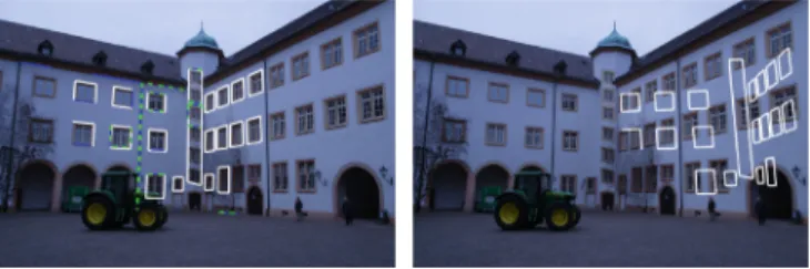
Fig. 1.Pose estimation results of OPnPL (left) and OPnP (right) in a scenario with a lack of reliable feature points. Blue points and solid line segments are detected in the image, and green dashed line segments are the model reference lines reprojected using the estimated pose. White lines are manually chosen on the 3D model to sketch its structure and projected onto the image to deem the quality of the estimated pose. Note also the shift along the line direction between the detected and the model lines. This issue needs to be handled in practice, where the reference lines in the model may
only be partially detected on the image (due to partial occlusions). Images from [41].
n = {3,4,5} [7,11,12,15,19,42]. The proliferation of feature point detec-tors [16,36] and descriptors [3,26,29,37,40] able to consistently retrieve many feature points per image, brought a series of new PnP algorithms that could efficiently handle arbitrarily large sets of points [9,13,18,24,25,27,30,38,45]. Amongst them, it is worth highlighting the EPnP [24], the first of these ‘effi-cient’ PnP solutions, and the OPnP [45], one of the most recent and accurate alternatives.
However, there are situations were PnP algorithms are likely to perform poorly because the presence of repetitive patterns or a lack of texture makes it difficult to reliably estimate and match feature points. This occurs, for instance, in man-made structures such as that shown in Fig.1. In these cases, though, one can still rely on other geometric primitives like straight lines, and compute camera pose using the so-called Perspective-n-Line (PnL) algorithms. Unfortu-nately, existing solutions are not yet as accurate as the point based approaches. The main problem to tackle in the PnL is that even when one may know 3D-to-2D line correspondences, there still can exist a shift of the lines along their direction. Additionally, the line may only be partially observed due to occlusions or misdetections (see again Fig.1).
In this paper, we propose a formulation of the PnL problem which is robust to partial and shifted line observations. At the core of our approach lies a para-meterization of the algebraic line segment reprojection error, that is linear on the segment endpoints. This parameterization, in turn, can be naturally integrated within the formulation of the original EPnP and OPnP algorithms, hence, allow-ing these PnP methods to leverage information about line correspondences with an almost negligible extra computation. We denote these joint line and point for-mulations as EPnPL and OPnPL, and through an exhaustive experimentation, show that they consistently improve the point only, and line only formulations.
2
Related Work
Most camera pose estimation algorithms are based on either point or line corre-spondences. Only a few works exploit lines’ and points’ projections simultane-ously. We next review the main related work in each of these categories. Pose from Points (PnP). The most standard approach for pose estimation considers 3D-to-2D point correspondences. Early PnP approaches addressed the minimal cases, with solutions for the P3P [6,12,14,21], P4P [4,11] and n = {4,5} [42]. These solutions, however, were by construction unable to handle larger amounts of points, or if they could, they were computationally demanding. Arbitrary number of points can be handled by the Direct Linear Transformation (DLT) [1], which however, estimates the full projection matrix without exploiting the fact that the internal parameters of the camera are known. This knowledge is shown to improve the pose estimation in more recent PnP approaches focused on building efficient solutions for the overconstrained case [2,10,18,20,24,32,45]. Amongst these, the EPnP [24] was the firstO(n) solution. Its main idea was to represent the 3D point coordinates as a linear combination of four control points, which became the only unknowns of the problem, independently of the total number of 3D coordinates. These control points were then retrieved using simple linearization techniques. This linearization has been subsequently substituted by polynomial solvers in the Robust PnP (RPnP) [25], the Direct Least Squares DLS [18], and the Optimal PnP (OPnP) [45], the most accurate of all PnP solutions. OPnP, draws inspiration on the DLS, but by-passes a degeneracy singularity of the DLS on the rotation by using a quaternion parameterization that allows to directly estimate the pose using a Gr¨obner basis solver.
Pose from Lines (PnL).The number of PnL algorithms is considerably smaller than the point-based ones. Back in the 90’s, closed-form approaches for the min-imal case with 3 line correspondences were proposed [5,7], together with theoret-ical studies about the multiple solutions this problem could have [31]. The DLT was shown to be applicable to line representations in [17], although again, with poorer results than algorithms that explicitly exploited the knowledge of the internal parameters of the camera, like [2], also applied to lines. [28] estimates the camera rotation matrix by solving a polynomial system of equations using an eigen decomposition of a so-called multiplication matrix. This method has been recently extended to full pose estimation (rotation+translation) in [33], by combining Pluecker 3D line parameterization with a DLT-like estimation algo-rithm. [44] combines the former P3L algorithms to compute pose by optimizing a cost function built from line triplets. Finally, [23] shows promising results by formulating the problem in terms of a system of symmetric polynomials. Pose from Points and Lines (PnPL). There is a very limited number of approaches that can simultaneously process point and line correspondences. The first of these approaches is the aforementioned DLT, initially used for point based pose estimation [1], and later extended to lines [17]. Both formulations can be integrated into the same framework. [8] also claims a methodology that can
potentially handle points and lines. Unfortunately, this is not theoretically shown neither demonstrated in practice. Finally, there are a few works that tackle the camera pose estimation from minimal number of points and lines. [35] proposes solutions for the P3L, P2L1P, P1L2P and P3L. And most recently, [22] solves for pose and focal length from points, directions and points with directions.
3
Our Approach to Pose from Points and Lines
Our approach to pose estimation holds on a new formulation of the straight line projection error, which allows incorporating information about the matched line segments into the PnP method, and in particular, into the EPnP and OPnP. This will result in two new algorithms for pose estimation from point and line correspondences, denoted as EPnPL and OPnPL.
3.1 Problem Formulation
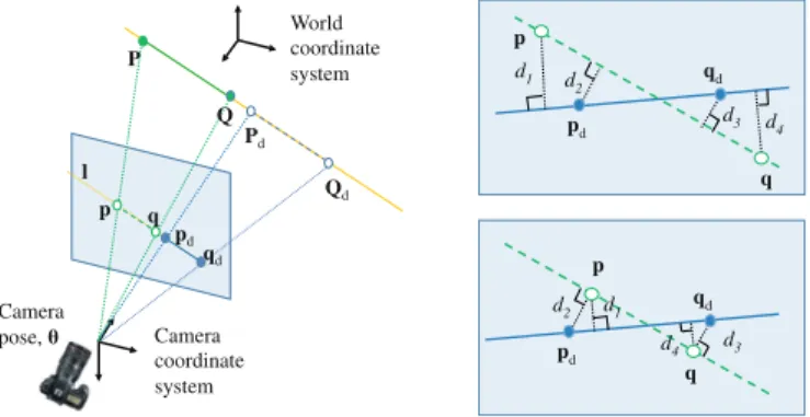
We are given n correspondences between 3D reference lines and 2D segment projections. 3D lines are represented by 3D endpoints{Pi,Qi}and 2D detected segments by 2D endpoints{pid,qid}, fori= 1, . . . , n. The camera is assumed to be calibrated, beingKthe matrix of internal parameters. Our goal is to estimate the rotationRand translationtthat align the camera and the world coordinate frames. It is worth pointing out that 2D line segment endpoints pi
d,qid do not
necessarily correspond to the projectionspi,qi of the 3D line endpointsPi,Qi. They are, instead, projections of some pointsPi
d,Qid lying on the same 3D line
as Pi,Qi (see Fig.2-left). This reflects the fact that in practice 3D reference lines may not be fully detected in the image or they can be partially occluded, precluding the use of point-based PnP algorithms.
3.2 General Definition of Line Segment Projection Error
Let the vector θ denote the pose parameters (R and t) of the calibrated cam-era. In the PnP formulation, we minimize the reprojection error of a projection function ˜x = π(θ,X), where ˜x ∈ R3 are the homogeneous coordinates of the 3D pointXprojected on the camera. Since we assume the calibration matrixK is known, we can pre-multiply the homogeneous image plane coordinates of the detected lines and points byK−1prior to solving the PnPL problem. In the rest
of this document, we will therefore assume that the homogeneous coordinates are normalized and thatKis a identity matrix.
In order to extend the point-based formulation to handle line segments, we need to formalize the reprojection error for lines. For that, let ˜pi
d,˜qid∈R3be the
homogeneous coordinates of the detected 2D endpoints pi
d,qid for the i-th line
segment. We represent this projected segment by its normalized line coefficients: ˆli= ˜pi d×q˜id, li= ˆli |ˆli| ∈R 3 . (1)
P Pd Qd p q pd l Camera coordinate system World coordinate system pd qd p q d1 d4 d3 d2 qd Q pd qd q d1 d4 d3 d2 p Camera pose,
Fig. 2. Left: Notation and problem formulation. Given a set of 3D-to-2D line
cor-respondences, we seek to estimate the pose θ that aligns the camera and the world
coordinate systems. 3D lines are represented by 3D endpoint pairs (P,Q). 2D
corre-sponding segments are represented by the detected endpoints (pd,qd) in the image
plane. Note that the 3D-to-2D line correspondence does not imply a correspondence of
the endpoints, preventing the use of a standard PnP algorithm.Right:Correction of
3D line segments to put in correspondence the projection of the line endpoints (P,Q)
with the detected segment endpoints (pd,qd). Top: before correction. Bottom: after
correction. Note how the projections (p,q) have been shifted along the line.
We then define thealgebraic point-line errorEplfor a 3D pointPi to a detected
line segmentli as distance between the lineli and the 2D projection ofPi: Epl(θ,Pi,li) = (li)π(θ,Pi). (2)
We further define the algebraic line segment errorEl as the sum of squares of
the two point-line errors for the 3D line segment endpoints: El(θ,Pi,Qi,li) = E2pl(θ,Pi,li) + E
2
pl(θ,Qi,li). (3)
The overall line segment error Elines for the whole image is the accumulated
algebraic line segment error over all the matched line segments: Elines(θ,{Pi},{Qi},{li}) =
i
El(θ,Pi,Qi,li). (4)
Note that this error does not explicitly use the detected line segment endpoints, depending only on the line coefficientsli. However, we seek to approximate with it the distance between the detected endpoints and the line projected from the model onto the image plane. This approximation may incur in gross errors in situations such as the one depicted in Fig.2-top-right. In this scenario, the true projected endpoints (p,q) are relatively far from the 2D detected endpoints (pd,qd), and the algebraic point-line errors d1 and d4 are much larger than
the gold standard errors d2, d3. This leads to preferred minimization of the
algebraic error for line matches where the detected and projected endpoints are further away. To handle this problem we considered a two-step approach. We first
estimate the initial camera pose with the given 3D model. We then recompute the position of the end-points onto the 3D model such that they reduce the distances between the projected and detected endpoints. Using this updated 3D model, we compute the final estimate of the camera pose. Figure2-bottom-right shows how the ground truth projected end-points have changed their position after having updated the 3D model. We next describe in more detail this correction process. 3.3 Putting 3D and 2D Line Endpoints in Correspondence
Let’s consider d be the length of the detected line segment and the notation detailed in Fig.2-right. After the first iteration of the complete PnPL algorithm (see Sects.3.4 and 3.5) we obtain an initial estimate of the camera pose. We then shift the endpoints of every line segment in the camera coordinate frame so that the length of the projected line segment matches the length of the detected segments, and the sum of distances between corresponding endpoints is minimal. More specifically, given an estimate for the poseR,t, we compute p,q and the unit line direction vector v along the projected lineˆl. We then shift the position ofpand q along this line, such that they become as close as possible from pd,qd, and separated by a distance d. This can be expressed with the
following two equations, function of a shifting parameterγ:
pd=p+γv qd=p+ (γ+d)v (5)
which yields that γ=v12(pd+qd)−p
−d
2. Given γ we can then take the
right hand side of (5) as the new projections ofp,q, and backproject the position of the new endpointsP,Qin the camera and world coordinate frames.
To backproject a point from the image plane to a 3D line, we compute the intersection of the line of sight of the point with the 3D line as follows:
λ˜x=αX+βD, (6)
where ˜xare the point’s projection homogeneous coordinates, Xis the 3D point belonging to the line and D is the 3D line direction. Both X and D are expressed w.r.t. the camera coordinate frame. From this equation we see that s = [−λ, α, β] is orthogonal to the vectors [X(j), D(j), −˜x(j)], j = 1,2, whereX(j) corresponds to thej-th component of the vectorX. We employ the cross product operation to solve for sand then compute the 3D point position asX+αβD. This procedure turns to be very fast.
3.4 EPnPL
We next describe a necessary modification to the EPnP algorithm to simultane-ously considernppoint andnl line correspondences.
In the EPnP [24] the projection of a point on the camera plane is written as πEPnP(θ,P) =K
4
j=1
where αj are point-specific coefficients computed from the model and Ccj for j = 1, . . . ,4 are the unknown control point coordinates in the camera frame. Recall that we are considering normalized homogeneous coordinates, and hence we can set the calibration matrix K to be the identity matrix. We define our vector of unknowns asμ= [C1, C2, C3, C4]and then obtain, using (2), an expression for the algebraic point-line error in case of EPnP:
Epl, EPnP(θ,Pi,li) = 4 j=1 αj(li)Ccj = (mil(Pi))μ, (8) formi
l(Pi) = ([α1, α2, α3, α4]⊗li). The overall error in Eq.4then becomes
Elines(θ,{Pi},{Qi},{li}) =
i
(mil(Pi))μ2+(mil(Qi))μ2. (9) Finally, considering both point and lines correspondences, the function to be minimized by the EPnPL will be
arg min µ Mpμ2+ Elines(θ,{Pi},{Qi},{li}) = arg min µ ¯Mμ2 (10)
where ¯M= [Mp, Ml ] ∈R2(np+nl)×12,Mp∈R2np×12 is the matrix of parameters
for thenppoint correspondences, as in [24], andMl∈R2nl×12is the matrix
cor-responding to the point-line errors of thenlmatched line segments. Equation10
is finally minimized by following the EPnP methodology. 3.5 OPnPL
In OPnP [45], the camera parameters are represented as^R=λ1¯R,ˆt=λ1¯t, where
¯
λis an average point depth in the camera frame. To deal with points and lines we define ¯λ as the average depth of the points and line segments’ endpoints. Similarly, we compute the mean point ¯Q, which can be used to write the third component of ˆt:
ˆ
t3= 1−ˆr3Q¯, (11)
whereˆr3 is the third row of ^R. The projection of a 3D pointX onto the image
plane (assuming the calibration matrixKto be the identity) will be:
πOPnP(θ,X) =^RX+ˆt. (12)
As we did for the EPnP, we use this projection into Eq.2to compute the algebraic point-line error.
Following [45], we can use Eq.11for ˆt3 to compute the algebraic error for all
points Epoints as a function of^R,ˆt1,ˆt2:
whereˆris a vectorized form of^R,ˆt12= [ˆt1tˆ2],Gp∈R2np×9 and Hp∈R2np×2
are matrices built from the projections and 3D model coordinates of the np
points, andkp is a 2npconstant vector.
The overall line segment error Elines as defined in Eq.4 can be expressed in
the same form as in Eq.13withGl,Hl,klinstead ofGp,Hp,kp, and using algebraic
line segment error (3) with (12) as point-line projection function.
In order to compute the pose, we adapt the cost function of [45] to the following one with both points and lines terms:
Etot(ρ,ˆt) = Epoints(ˆr(ρ),ˆt) + Elines(ˆr(ρ),ˆt), (14)
where we parameterizeˆrwith non-unit quaternions vectorρ= [a, b, c, d]. We next seek to minimize this function w.r.t. the pose parameters.
Setting the derivative of Etotw.r.t.ˆtto zero, and denotingGtot= [Gp, Gl ],
Htot= [Hp, Hl ],ktot= [kp, kl ] we can writeˆtas a function ofˆr:
H
tot(Gtotˆr+Htotˆt+ktot) = 0 =⇒ ˆt=Pˆr+u, (15)
forP=−(HtotHtot)−1(HtotGtot),u=−(HtotHtot)−1Htotktot.
The derivative of Etot w.r.t. the first quaternion parameterais:
∂ˆr ∂aG
tot(Gtotˆr+Htotˆt+ktot) = ∂
ˆr ∂aG
tot
(Gtot+HtotP)ˆr+Htotu+ktot
= 0, (16) where in the second step we have used Eq.15. Three more equations analogous to (16) constitute a system which the original OPnP uses to design a specific polynomial solver [45]. In our case we can use exactly the same solver, as the equations we get for joint point and line matches, have exactly the same form as when only considering points.
4
Experiments
We evaluate the proposed approach in “points and lines” and “only lines” situa-tions, nonplanar and planar configurasitua-tions, and synthetic and real experiments. 4.1 Synthetic Experiments
We will compare our approach against state-of-the-art in two situations: A joint point-and-line case, and a line-only case. In both scenarios we will consider non-planar and non-planar configurations, and will report rotation and translation errors for increasing amounts of 2D noise and number of correspondences. We will also study the influence of the amount of shift between the lines in the 3D model, and the observed segments projected on the image.
In the synthetic experiments we assume a virtual 640×480 pixels calibrated camera with focal length of 500. We randomly generatenp+ 2nl 3D points in
(a) Nonplanar: PnP (np= 6), PnL (nl= 10), PnPL (np= 6,nl= 10 )
0 0.5 1 1.5 2 2.5 3 3.5 4 Noise, std.dev. (pix.) 0
0.5 1 1.5
Rotation Error (degrees)
Median Rotation
0 0.5 1 1.5 2 2.5 3 3.5 4 Noise, std.dev. (pix.) 0
2 4 6
Rotation Error (degrees)
Mean Rotation
0 0.5 1 1.5 2 2.5 3 3.5 4 Noise, std.dev. (pix.) 0 0.5 1 1.5 2 Translation Error (%) Median Translation 0 0.5 1 1.5 2 2.5 3 3.5 4 Noise, std.dev. (pix.) 0 1 2 3 4 5 Translation Error (%) Mean Translation Mirzaei RPnL Pluecker EPnP_GN OPnP DLT EPnPL OPnPL OPnP* (b) Nonplanar: PnP (np= 10), PnL (nl= 10), PnPL (np=nl= 5 ) 0 0.5 1 1.5 2 2.5 3 3.5 4 Noise, std.dev. (pix.) 0
0.5 1 1.5
Rotation Error (degrees)
Median Rotation
0 0.5 1 1.5 2 2.5 3 3.5 4 Noise, std.dev. (pix.) 0
2 4 6
Rotation Error (degrees)
Mean Rotation
0 0.5 1 1.5 2 2.5 3 3.5 4 Noise, std.dev. (pix.) 0 0.5 1 1.5 2 Translation Error (%) Median Translation 0 0.5 1 1.5 2 2.5 3 3.5 4 Noise, std.dev. (pix.) 0 1 2 3 4 5 Translation Error (%) Mean Translation Mirzaei RPnL Pluecker EPnP_GN OPnP DLT EPnPL OPnPL OPnP* (c) Planar: PnP (np= 6), PnL (nl= 10), PnPL (np= 6,nl= 10 ) 0 0.5 1 1.5 2 2.5 3 3.5 4 Noise, std.dev. (pix.) 0
0.5 1 1.5
Rotation Error (degrees)
Median Rotation
0 0.5 1 1.5 2 2.5 3 3.5 4 Noise, std.dev. (pix.) 0
2 4 6
Rotation Error (degrees)
Mean Rotation
0 0.5 1 1.5 2 2.5 3 3.5 4 Noise, std.dev. (pix.) 0 0.5 1 1.5 2 Translation Error (%) Median Translation 0 0.5 1 1.5 2 2.5 3 3.5 4 Noise, std.dev. (pix.) 0 1 2 3 4 5 Translation Error (%) Mean Translation Mirzaei RPnL EPnP_Planar_GN OPnP DLT_Planar EPnPL_Planar OPnPL OPnP* (d) Planar: PnP (np= 10), PnL (nl= 10), PnPL (np=nl= 5 ) 0 0.5 1 1.5 2 2.5 3 3.5 4 Noise, std.dev. (pix.) 0
0.5 1 1.5
Rotation Error (degrees)
Median Rotation
0 0.5 1 1.5 2 2.5 3 3.5 4 Noise, std.dev. (pix.) 0
2 4 6
Rotation Error (degrees)
Mean Rotation
0 0.5 1 1.5 2 2.5 3 3.5 4 Noise, std.dev. (pix.) 0 0.5 1 1.5 2 Translation Error (%) Median Translation 0 0.5 1 1.5 2 2.5 3 3.5 4 Noise, std.dev. (pix.) 0 1 2 3 4 5 Translation Error (%) Mean Translation Mirzaei RPnL EPnP_Planar_GN OPnP DLT_Planar EPnPL_Planar OPnPL OPnP*
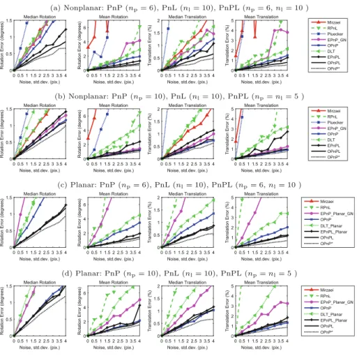
Fig. 3.Pose from point and line correspondences. Accuracy w.r.t. image noise level.
and nl are the number of points and line segments, respectively. We then build
a random rotation matrix; the translation vector is taken to be the mean vector of all the points, as done in [45]. From the last 2nl generated points, we formnl
pairs, which will be the 3D reference segments (Pand Qin Fig.2). Thenp3D
points and 2nl endpoints are then projected onto the image, and perturbed by
Gaussian noise. For each 3D line we generate two more points on the same line (Pd and Qd in Fig.2), by randomly shiftingPand Q, and project them onto
the image and corrupt with noise (pdandqd in Fig.2). In the following, unless
said otherwise, noise standard deviation is set to 1 pixel, the segment length is set to a uniformly random value within the interval [1.5, 4.5], and the segment shift is also taken randomly within [−2, 2].
In all quantitative results, we will provide the absolute error (in degrees) for rotation, and the relative error (%) for translation. All plots are created by running 500 independent simulations and report the mean and median errors.
(a) Nonplanar: PnP (np), PnL(nl), PnPL (np, nl) 6 7 8 9 10 11 12 13 14 15 np, nl 0 0.5 1
Rotation Error (degrees)
Median Rotation 6 7 8 9 10 11 12 13 14 15 np, nl 0 0.5 1
Rotation Error (degrees)
Mean Rotation 6 7 8 9 10 11 12 13 14 15 np, nl 0 0.5 1 1.5 Translation Error (%) Median Translation 6 7 8 9 10 11 12 13 14 15 np, nl 0 0.5 1 1.5 2 Translation Error (%) Mean Translation Mirzaei RPnL Pluecker EPnP_GN OPnP DLT EPnPL OPnPL OPnP* (b) Nonplanar: PnP (np), PnL (nl), PnPL (np=nl= 0.5np= 0.5nl) 6 7 8 9 10 11 12 13 14 15 np,nl 0 0.5 1 1.5
Rotation Error (degrees)
Median Rotation 6 7 8 9 10 11 12 13 14 15 np,nl 0 2 4 6
Rotation Error (degrees)
Mean Rotation 6 7 8 9 10 11 12 13 14 15 np,nl 0 0.5 1 1.5 2 Translation Error (%) Median Translation 6 7 8 9 10 11 12 13 14 15 np,nl 0 1 2 3 4 5 Translation Error (%) Mean Translation Mirzaei RPnL Pluecker EPnP_GN OPnP DLT EPnPL OPnPL OPnP* (c) Planar: PnP (np), PnL(nl), PnPL (np, nl) 6 7 8 9 10 11 12 13 14 15 np, nl 0 0.5 1 1.5
Rotation Error (degrees)
Median Rotation 6 7 8 9 10 11 12 13 14 15 np, nl 0 2 4 6
Rotation Error (degrees)
Mean Rotation 6 7 8 9 10 11 12 13 14 15 np, nl 0 0.5 1 1.5 2 Translation Error (%) Median Translation 6 7 8 9 10 11 12 13 14 15 np, nl 0 1 2 3 4 5 Translation Error (%) Mean Translation Mirzaei RPnL EPnP_Planar_GN OPnP DLT_Planar EPnPL_Planar OPnPL OPnP* (d) Planar: PnP (np), PnL (nl), PnPL (n p=nl= 0.5np= 0.5nl) 7 9 11 13 15 n p,nl 0 0.5 1 1.5
Rotation Error (degrees)
Median Rotation 7 9 11 13 15 n p,nl 0 2 4 6
Rotation Error (degrees)
Mean Rotation 7 9 11 13 15 n p,nl 0 0.5 1 1.5 2 Translation Error (%) Median Translation 7 9 11 13 15 n p,nl 0 1 2 3 4 5 Translation Error (%) Mean Translation Mirzaei RPnL EPnP_Planar_GN OPnP DLT_Planar EPnPL_Planar OPnPL OPnP*
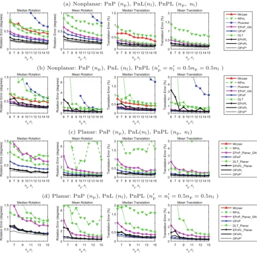
Fig. 4.Pose from point and line correspondences. Accuracy w.r.t. increasing number of point or line correspondences.
Regarding state-of-the-art, we compare against the following PnL algorithms: RPnL [44], Mirzaei [28] and Pluecker [33]. As for PnP methods we will include EPnP [24] and OPnP [45]; and the DLT proposed in [17] for the PnPL. Our two approaches will be denoted as EPnPL and OPnPL. Additionally, we will also consider the OPnP*, which will take as input both point and line corre-spondences. However, for the lines we will consider the true correspondences {Pi,Qi} ↔ {pi,qi} instead of the correspondences {Pi,Qi} ↔ {pi
d,qid} (see
again Fig.2), that feed our two approaches and the rest of algorithms. Note that this is an unrealistic situation, and OPnP* has to be interpreted as a baseline indicating the best performance one could expect.
Pose from Points and Lines. We consider point and line correspondences for two configurations, non-planar and planar. We evaluate the accuracy of the approaches w.r.t. the image noise in Fig.3, and w.r.t. an increasing number of
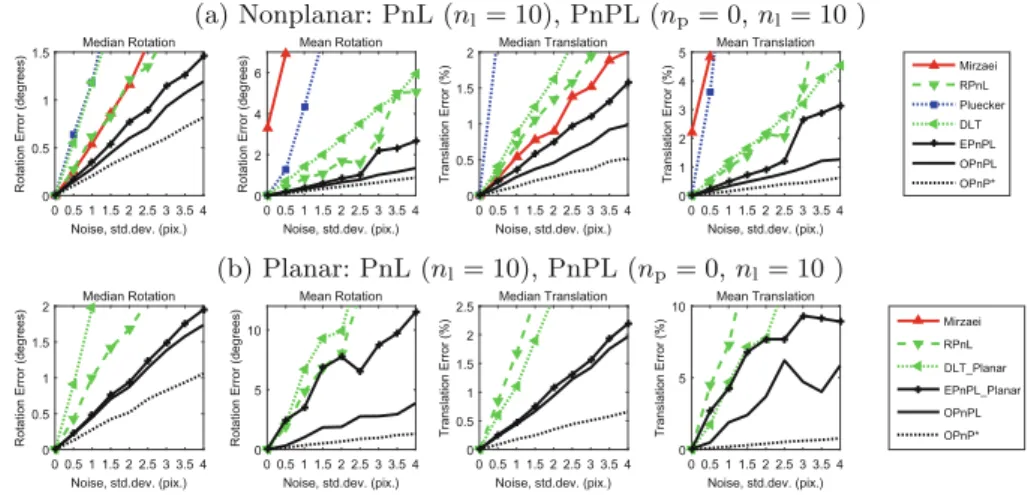
(a) Nonplanar: PnL (nl= 10), PnPL (np= 0,nl= 10 )
0 0.5 1 1.5 2 2.5 3 3.5 4 Noise, std.dev. (pix.) 0
0.5 1 1.5
Rotation Error (degrees)
Median Rotation
0 0.5 1 1.5 2 2.5 3 3.5 4 Noise, std.dev. (pix.) 0
2 4 6
Rotation Error (degrees)
Mean Rotation
0 0.5 1 1.5 2 2.5 3 3.5 4 Noise, std.dev. (pix.) 0 0.5 1 1.5 2 Translation Error (%) Median Translation 0 0.5 1 1.5 2 2.5 3 3.5 4 Noise, std.dev. (pix.) 0 1 2 3 4 5 Translation Error (%) Mean Translation Mirzaei RPnL Pluecker DLT EPnPL OPnPL OPnP* (b) Planar: PnL (nl= 10), PnPL (np= 0,nl= 10 ) 0 0.5 1 1.5 2 2.5 3 3.5 4 Noise, std.dev. (pix.) 0
0.5 1 1.5 2
Rotation Error (degrees)
Median Rotation
0 0.5 1 1.5 2 2.5 3 3.5 4 Noise, std.dev. (pix.) 0
5 10
Rotation Error (degrees)
Mean Rotation
0 0.5 1 1.5 2 2.5 3 3.5 4 Noise, std.dev. (pix.) 0 0.5 1 1.5 2 2.5 Translation Error (%) Median Translation 0 0.5 1 1.5 2 2.5 3 3.5 4 Noise, std.dev. (pix.) 0 5 10 Translation Error (%) Mean Translation Mirzaei RPnL DLT_Planar EPnPL_Planar OPnPL OPnP*
Fig. 5.Pose from only line correspondences. Accuracy w.r.t. image noise level.
correspondences (either points, lines or points and lines) in Fig.4. To ensure fairness between PnP, PnL and PnPL algorithms we analyze two situations: (a) Different number of constraints. When evaluating accuracy w.r.t. image noise we consider np = 6 point correspondences for the PnP algorithms (minimum
number required by EPnP), nl = 10 correspondences for the PnL (minimum
number for Pluecker [33]) and the PnPL methods usenp= 6 point plusnl= 10
line correspondences. The results for the non-planar and planar configurations are shown in Fig.3(a) and (c), respectively. As expected, the EPnPL and OPnPL methods are more accurate than the point only versions, because they are using additional information. Indeed, OPnPL is very close from the OPnP* base-line, indicating that line information is very well exploited. Additionally, our approaches work remarkably better than DLT (the other PnPL solution) and the rest of PnL methods. In Fig.4(a) and (c) we observe that the methods’ accuracy w.r.t. an increasing number of points also shows that our approaches exhibit the best performances.
(b) Constant number of constraints. We also provide results of accuracy w.r.t. noise in which we limit the total number of constraints, either obtained from line or point correspondences, to a constant value (np = 10 for PnP methods,
nl = 10 for PnL methods andnp= 5,nl= 5 for PnPL methods). Note that PnP
algorithms will be in this case in a clear advantage, as we are feeding them with point correspondences just perturbed by noise. PnL and PnPL algorithms need to deal with weaker line correspondences which besides noisy, are less spatially constrained. Results in Fig.3(b) and (d) confirm this. EPnP and OPnP have largely improved their performance compared to the previous scenario, but what is very remarkable is that OPnPL is almost as good as its point-only version OPnP. EPnPL is more clearly behind EPnP. In any event, our solutions again perform much better than DLT and the PnL algorithms. Similar performance patterns can be observed in Fig.4(b) and (d) when evaluating the accuracy
80 200 320 440 560 np+nl 0 0.02 0.04 0.06 0.08
Average Runtime (sec)
Time 20 220 420 620 np+nl 0 0.005 0.01 0.015 0.02 Time, s.
Mean processing time
20 220 420 620 np+nl 0 0.01 0.02 0.03 0.04 Time, s.
Mean solving time
Mirzaei RPnL Pluecker EPnP_GN OPnP DLT EPnPL OPnPL
Fig. 6.Running times for increasing number of correspondences. Left: All methods.
Center: Phases of our approaches. ‘Processing’ (center-left) includes the calculation of
2D line equations and the line correction from Sect.3.3. ‘Solving’ (center-right) refers
to the actual time taken to compute the pose as described in Sects.3.4and3.5.
w.r.t. number of constraints in the non-planar case. For the planar case, our two solutions clearly outperform all other approaches, specially in rotation error. Pose from Lines Only. In this experiment we just compare the line-based approaches, i.e., the PnL and PnPL methods (but only fed with line correspon-dences). We considernl= 10. In Fig.5(a) and (b) we show the pose accuracy at
increasing levels of noise, for the nonplanar and planar case. EPnPL and OPnPL perform consistently better than all other approaches, specially OPnPL. We also observed that PnL methods are very unstable under planar configurations and, in particular, Pluecker [33] did not manage to work and Mirzaei [28] yielded a very large error (out of bounds in the graphs).
Scalability.We evaluate the runtime of the methods for an increasing number of point and line correspondences. For the PnL and PnP methods we usednpandnl
correspondences, respectively, withnp=nl. The PnPL methods receive twice the
number of correspondences, i.e.,np+nl. Figure6-left shows the results, where all
methods are implemented in MATLAB. As expected, the runtime of OPnPL and EPnPL is about twice the runtime of their point-only counterparts, confirming they are still O(n) algorithms. This linear time is maintained even having to execute the correction scheme of the line segments described in Sect.3.3. For this to happen, our implementations exploit efficient vectorized operations. Figure6 -right reports the time taken by our approach at different phases.
0.1 0.3 0.5 0.7 0.9 Segment shift coeff. 0
0.5 1 1.5
Rotation Error (degrees)
Median Rotation
0.1 0.3 0.5 0.7 0.9 Segment shift coeff. 0
2 4 6
Rotation Error (degrees)
Mean Rotation
0.10.3 0.5 0.7 0.9 Segment shift coeff. 0 0.5 1 1.5 2 Translation Error (%) Median Translation 0.1 0.30.5 0.7 0.9 Segment shift coeff. 0 1 2 3 4 5 Translation Error (%) Mean Translation Mirzaei RPnL Pluecker DLT OPnP_naive EPnPL OPnPL OPnP*
Fig. 7. Robustness to the amount of shift between the 3D reference lines and the projected ones. See text for details.
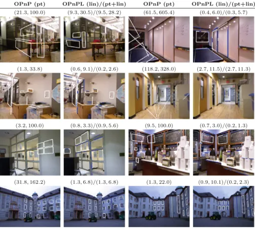
OPnP (pt) OPnPL (lin)/(pt+lin) OPnP (pt) OPnPL (lin)/(pt+lin)
(21.3,100.0) (9.3,30.5)/(9.5,28.2) (61.5,605.4) (0.4,6.0)/(0.3,5.7)
(1.3,33.8) (0.6,9.1)/(0.2,2.6) (118.2,328.0) (2.7,11.5)/(2.7,11.3)
(3.2,100.0) (0.8,3.3)/(0.9,5.6) (9.5,100.0) (0.7,3.0)/(0.2,1.3)
(31.8,162.2) (1.3,6.8)/(1.3,6.8) (1.3,22.0) (0.9,10.1)/(0.2,2.3)
Fig. 8. Pose estimation on the NYU2 and Castle (last row) datasets, for OPnP and OPnPL. The numbers on top of each image indicate the rotation and translation error as pairs (Rot. Err. (deg), Translation Error (%)). For the OPnPL we report both the error of the only line case, and of the case with joint points and lines. The lines of the 3D model are reprojected onto the images using the estimated pose. For the OPnPL we reproject the lines using the pose estimated using both points and lines.
Shift of Line Segments. As discussed above, to simulate real situations in which a 3D reference line on the model may only be partially projected onto the input image, we enforce the detected lines to be shifted versions of the true pro-jected lines. In this experiment, we evaluate the robustness of the PnL and PnPL algorithms to this shift, which is controlled by means of a parameter k∈[0,1]. k = 0 would correspond to a non-shift, i.e., {pi,qi} ={pi
d,qid}. k = 1 would
correspond to a shift of 3 units between the true projected and the detected line endpoints. Additionally, we consider another baseline, the OPnP naive, where we feed the OPnP algorithm with the correspondences {Pi,Qi} ↔ {pi
d,qid}.
The results are shown in Fig.7. Note that PnL methods and DLT are insensitive to the amount of shift (Mirzaei [28] occasionally fails, but this is independent on the amount of shift). This was expected, as these algorithms only consider the
line directions in the image plane, and not the particular position of the lines. Our EPnPL and OPnPL approaches could be more sensitive, as we explicitly use the position of the line in the image plane. However, the correction step we use in Sect.3.3gets rid of this problem. As expected OPnP naive fails completely. 4.2 Real Images
We also evaluated our approach on real images of the NYU2 [39] and EPFL Castle-P19 [41] datasets. These are datasets with structured objects (indoor and man-made scenarios) and with a large amount of straight lines and repetitive patterns that will benefit of a joint point and line based approach. For these experiments we will only evaluate the point based OPnP and the OPnPL, either using only lines or lines with points.
We implemented a standard structure from motion pipeline on triplets of images for building the 3D models. Details are provided in the supplemental material. One of the images of the triplet is then taken to be the reference and another the test image. SIFT feature points are detected in both images and line features are detected and represented using the recent scale invariant line descriptor [43], shown to be adequate for wide baseline matching. The test image is matched against the model, using RANSAC with P3P for the point-only case; and using RANSAC with OPnPL for a combination of four points or lines (4 lines, 3 lines/1 point, etc.) The final pose is computed using the points within the consensus for the OPnP. For the OPnPL we consider the concensus made of both points and lines and the concensus made of only lines.
Figure8reports sample images of both datasets, including both quantitative and qualitative results. As can be seen, these type of scenarios (repetitive pat-terns in the castle, many straight and planar surfaces, low textured areas), are situations in which the point-based approaches are prone to fail, and where lines and lines+points methods perform more robustly.
5
Conclusion
In this paper we have proposed an approach to integrate 3D-to-2D line correspon-dences within the formulation of two state-of-the-art PnP algorithms, allowing them to indistinctly treat points, lines or a combination of them. In order to do so, we introduce an algebraic line error that is formulated in terms of the line endpoints and which is robust to large shifts between their 3D positions and its 2D projection. This reproduces the situation that occurs in practice, where 3D model lines are just partially observed in the image due to occlusions or mis-detections. We extensively evaluate our algorithms on both synthetic and real images, showing a boost in performance w.r.t. other approaches, either those that only use lines, points or a combination of both. Additionally, our approach retains the O(n) capabilities of the PnP algorithms we build upon, making them appropriate for real time computations in structure-from-motion frameworks, that since to date have mostly exploited point correspondences. We plan to explore this line in the near future.
References
1. Abdel-Aziz, Y.: Direct linear transformation from comparator coordinates in close-range photogrammetry. In: ASP Symposium on Close-Range Photogrammetry in Illinois, 1971 (1971)
2. Ansar, A., Daniilidis, K.: Linear pose estimation from points or lines. IEEE Trans.
Pattern Anal. Mach. Intell.25(5), 578–589 (2003)
3. Bay, H., Tuytelaars, T., Gool, L.: SURF: speeded up robust features. In: Leonardis, A., Bischof, H., Pinz, A. (eds.) ECCV 2006. LNCS, vol. 3951, pp. 404–417. Springer,
Heidelberg (2006). doi:10.1007/11744023 32
4. Bujnak, M., Kukelova, Z., Pajdla, T.: A general solution to the P4P problem for camera with unknown focal length. In: IEEE Conference on Computer Vision and Pattern Recognition, 2008, CVPR 2008, pp. 1–8. IEEE (2008)
5. Chen, H.H.: Pose determination from line-to-plane correspondences: existence con-dition and closed-form solutions. In: Third International Conference on Computer Vision, 1990, Proceedings, pp. 374–378. IEEE (1990)
6. DeMenthon, D., Davis, L.S.: Exact and approximate solutions of the
perspective-three-point problem. IEEE Trans. Pattern Anal. Mach. Intell.11, 1100–1105 (1992)
7. Dhome, M., Richetin, M., Lapreste, J.T., Rives, G.: Determination of the attitude of 3D objects from a single perspective view. IEEE Trans. Pattern Anal. Mach.
Intell.11(12), 1265–1278 (1989)
8. Ess, A., Neubeck, A., Van Gool, L.J.: Generalised linear pose estimation. In: BMVC, pp. 1–10 (2007)
9. Ferraz, L., Binefa, X., Moreno-Noguer, F.: Very fast solution to the PnP problem with algebraic outlier rejection. In: Proceedings of the Conference on Computer Vision and Pattern Recognition (CVPR), pp. 501–508 (2014)
10. Fiore, P.D.: Efficient linear solution of exterior orientation. IEEE Trans. Pattern
Anal. Mach. Intell.2, 140–148 (2001)
11. Fischler, M.A., Bolles, R.C.: Random sample consensus: a paradigm for model fitting with applications to image analysis and automated cartography. Commun.
ACM24(6), 381–395 (1981)
12. Gao, X.S., Hou, X.R., Tang, J., Cheng, H.F.: Complete solution classification for the perspective-three-point problem. IEEE Trans. Pattern Anal. Mach. Intell.
25(8), 930–943 (2003)
13. Garro, V., Crosilla, F., Fusiello, A.: Solving the PnP problem with anisotropic orthogonal procrustes analysis. In: 2012 Second International Conference on 3D Imaging, Modeling, Processing, Visualization and Transmission, pp. 262–269. IEEE (2012)
14. Grunert, J.A.: Das pothenotische problem in erweiterter gestalt nebst uber seine anwendungen in geoda sie. In: Grunerts Archiv fu Mathematik und Physik (1841)
15. Haralick, R.M., Lee, C.n., Ottenburg, K., N¨olle, M.: Analysis and solutions of the
three point perspective pose estimation problem. In: IEEE Computer Society Con-ference on Computer Vision and Pattern Recognition, 1991, Proceedings CVPR 1991, pp. 592–598. IEEE (1991)
16. Harris, C., Stephens, M.: A combined corner and edge detector. In: Alvey Vision Conference, Citeseer, vol. 15, p. 50 (1988)
17. Hartley, R., Zisserman, A.: Multiple View Geometry in Computer Vision. Cambridge University Press, Cambridge (2003)
18. Hesch, J.A., Roumeliotis, S.I.: A direct least-squares (DLS) method for PnP. In: 2011 IEEE International Conference on Computer Vision (ICCV), pp. 383–390. IEEE (2011)
19. Horaud, R., Conio, B., Leboulleux, O., Lacolle, L.B.: An analytic solution for the perspective 4-point problem. In: IEEE Computer Society Conference on Computer Vision and Pattern Recognition, 1989, Proceedings CVPR 1989, pp. 500–507. IEEE (1989)
20. Kneip, L., Li, H., Seo, Y.: UPnP: an optimal O(n) solution to the absolute
pose problem with universal applicability. In: Fleet, D., Pajdla, T., Schiele, B., Tuytelaars, T. (eds.) ECCV 2014. LNCS, vol. 8689, pp. 127–142. Springer,
Heidelberg (2014). doi:10.1007/978-3-319-10590-1 9
21. Kneip, L., Scaramuzza, D., Siegwart, R.: A novel parametrization of the perspective-three-point problem for a direct computation of absolute camera posi-tion and orientaposi-tion. In: 2011 IEEE Conference on Computer Vision and Pattern Recognition (CVPR), pp. 2969–2976. IEEE (2011)
22. Kuang, Y., Astrom, K.: Pose estimation with unknown focal length using points, directions and lines. In: Proceedings of the IEEE International Conference on Com-puter Vision, pp. 529–536 (2013)
23. Kuang, Y., Zheng, Y., Astrom, K.: Partial symmetry in polynomial systems and its applications in computer vision. In: Proceedings of the IEEE Conference on Computer Vision and Pattern Recognition, pp. 438–445 (2014)
24. Lepetit, V., Moreno-Noguer, F., Fua, P.: EPnP: an accurate O(n) solution to the
PnP problem. Int. J. Comput. Vis.81(2), 155–166 (2009)
25. Li, S., Xu, C., Xie, M.: A robust O(n) solution to the perspective-n-point problem.
IEEE Trans. Pattern Anal. Mach. Intell.34(7), 1444–1450 (2012)
26. Lowe, D.G.: Distinctive image features from scale-invariant keypoints. Int. J.
Com-put. Vis.60(2), 91–110 (2004)
27. Lu, C.P., Hager, G.D., Mjolsness, E.: Fast and globally convergent pose estimation
from video images. IEEE Trans. Pattern Anal. Mach. Intell.22(6), 610–622 (2000)
28. Mirzaei, F.M., Roumeliotis, S., et al.: Globally optimal pose estimation from line correspondences. In: 2011 IEEE International Conference on Robotics and Automation (ICRA), pp. 5581–5588. IEEE (2011)
29. Moreno-Noguer, F.: Deformation and illumination invariant feature point descrip-tor. In: 2011 IEEE Conference on Computer Vision and Pattern Recognition (CVPR), pp. 1593–1600. IEEE (2011)
30. Nakano, G.: Globally optimal DLS method for PnP problem with Cayley para-meterization. In: Proceedings of British Machine Vision Conference 2015. BMVA (2015)
31. Navab, N., Faugeras, O.: Monocular pose determination from lines: critical sets and maximum number of solutions. In: 1993 IEEE Computer Society Conference on Computer Vision and Pattern Recognition, 1993, Proceedings CVPR 1993, pp. 254–260. IEEE (1993)
32. Penate-Sanchez, A., Andrade-Cetto, J., Moreno-Noguer, F.: Exhaustive lineariza-tion for robust camera pose and focal length estimalineariza-tion. IEEE Trans. Pattern Anal.
Mach. Intell.10, 2387–2400 (2013)
33. Pribyl, B., Zemk, P.,et al.: Camera pose estimation from lines using Pl¨ucker
coor-dinates. In: Proceedings of British Machine Vision Conference 2015. BMVA (2015) 34. Quan, L., Lan, Z.: Linear n-point camera pose determination. IEEE Trans. Pattern
Anal. Mach. Intell.21(8), 774–780 (1999)
35. Ramalingam, S., Bouaziz, S., Sturm, P.: Pose estimation using both points and lines for geo-localization. In: 2011 IEEE International Conference on Robotics and Automation (ICRA), pp. 4716–4723. IEEE (2011)
36. Rosten, E., Drummond, T.: Machine learning for high-speed corner detection. In: Leonardis, A., Bischof, H., Pinz, A. (eds.) ECCV 2006. LNCS, vol. 3951, pp. 430–
443. Springer, Heidelberg (2006). doi:10.1007/11744023 34
37. Rublee, E., Rabaud, V., Konolige, K., Bradski, G.: ORB: an efficient alternative to SIFT or SURF. In: 2011 IEEE International Conference on Computer Vision (ICCV), pp. 2564–2571. IEEE (2011)
38. Schweighofer, G., Pinz, A.: Globally optimal O(n) solution to the PnP problem for general camera models. In: BMVC, pp. 1–10 (2008)
39. Silberman, N., Hoiem, D., Kohli, P., Fergus, R.: Indoor segmentation and support inference from RGBD images. In: Fitzgibbon, A., Lazebnik, S., Perona, P., Sato, Y., Schmid, C. (eds.) ECCV 2012. LNCS, vol. 7576, pp. 746–760. Springer, Heidelberg
(2012). doi:10.1007/978-3-642-33715-4 54
40. Simo-Serra, E., Trulls, E., Ferraz, L., Kokkinos, I., Fua, P., Moreno-Noguer, F.: Discriminative learning of deep convolutional feature point descriptors. In: Pro-ceedings of the International Conference on Computer Vision (ICCV) (2015) 41. Strecha, C., von Hansen, W., Gool, L.V., Fua, P., Thoennessen, U.: On
benchmark-ing camera calibration and multi-view stereo for high resolution imagery. In: IEEE Conference on Computer Vision and Pattern Recognition, 2008, CVPR 2008, pp. 1–8. IEEE (2008)
42. Triggs, B.: Camera pose and calibration from 4 or 5 known 3D points. In: The Proceedings of the Seventh IEEE International Conference on Computer Vision, 1999, vol. 1, pp. 278–284. IEEE (1999)
43. Verhagen, B., Timofte, R., Van Gool, L.: Scale-invariant line descriptors for wide baseline matching. In: 2014 IEEE Winter Conference on Applications of Computer Vision (WACV), pp. 493–500. IEEE (2014)
44. Zhang, L., Xu, C., Lee, K.-M., Koch, R.: Robust and efficient pose estimation from line correspondences. In: Lee, K.M., Matsushita, Y., Rehg, J.M., Hu, Z. (eds.)
ACCV 2012. LNCS, vol. 7726, pp. 217–230. Springer, Heidelberg (2013). doi:10.
1007/978-3-642-37431-9 17
45. Zheng, Y., Kuang, Y., Sugimoto, S., Astrom, K., Okutomi, M.: Revisiting the PnP problem: a fast, general and optimal solution. In: 2013 IEEE International Conference on Computer Vision (ICCV), pp. 2344–2351. IEEE (2013)