“Soft” policing at hot spots—do police community support officers work? A randomized controlled trial

B

Soft

^

policing at hot spots

—

do police community

support officers work? A randomized controlled trial

Barak Ariel1,2&Cristobal Weinborn1&

Lawrence W Sherman1,3

Published online: 21 May 2016

#The Author(s) 2016. This article is published with open access at Springerlink.com

Abstract

ObjectivesTo determine whether crime-reduction effects of increased police patrols in hot spots are dependent on theBhard^threat of immediate physical arrest, or whether

Bsoft^patrols by civilian (but uniformed) police staff with few arrest powers and no weapons can also reduce crime. We also sought to assess whether the number of discrete patrol visits to a hot spot was more or less important than the total minutes of police presence across all visits, and whether effects based on counts of crime would be consistent with effects on a Crime Harm Index outcome.

Methods We randomly assigned 72 hot spots into 34 treatment units and 38 controls. Treatment consisted of increases in foot patrol by uniformed, unarmed, Police Community Support Officers (PCSOs) who carry no weapons and hold few arrest powers beyond those of ordinary citizens. GPS-trackers on every PCSO and Constable in the city yielded precise measurements of all patrol time in all hot spots. Standardized mean differences (Cohen’s d), OLS regression model, and Weighted Displacement Quotient are used to assess main effects, to model the interaction effect of GPS data with treatment, and to measure the diffusion-of-benefits of the intervention, respective-ly. Outcomes included counts of incidents as well as the Cambridge Crime Harm Index. ResultsAs intended, patrol visits and minutes by Police Constables were equal across the treatment and control groups. The sole difference in policing between the treatments groups was in visits to the hot spots by PCSOs, in both the mean daily frequency of discrete visits (T = 4.65, C = 2.66;p≤.001) and total minutes across all visits (T = 37.41,

* Barak Ariel

[email protected]; [email protected]

1

Institute of Criminology, University of Cambridge, Sidgwick Avenue, Cambridge CB3 9DA, UK

2 _{Institute of Criminology, Faculty of Law, Hebrew University, Mount Scopus,}

Jerusalem 91905, Israel

3

Department of Criminology and Criminal Justice, University of Maryland, 2220 Samuel J. LeFrak Hall, College Park, MD 20742, USA

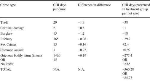
C = 15.92; p≤.001), approximately two more ten-minute visits per day in treatment than in control. Main effect estimates suggest 39 % less crime by difference-in-difference analysis of reported crimes compared to control conditions, and 20 % reduc-tions in emergency calls-for-service compared to controls. Crime in surrounding areas showed a diffusion of benefits rather than displacement for treatment hot spots compared to controls. A BReiss’s Reward^ effect was observed, with more proactive patrols predicting less crime across treatment hot spots, while more reactive PCSO time predicted more crime across control hot spots. Crime Harm Index estimates of the seriousness value of crime prevented ranged from 85 to 360 potential days of imprisonment in each treatment group hot spot (relative to controls) by a mean difference of 21 more minutes of PCSO patrol per day, for a potential return on investment of up to 26 to 1.

Conclusions A crime reduction effect of extra patrols in hot spots is not conditional on

Bhard^police power. Even small differences in foot patrols showing theBsoft power^of unarmed paraprofessionals, holding constant vehicular patrols by Police Constables, were causally linked to both lower counts of crimes and a substantially lower crime harm index score. Correlational evidence within the treatment group suggests that greater frequency of discrete PCSO visits may yield more crime reduction benefit than greater duration of those visits, but RCTs are needed for better evidence on this crucial issue. Keywords Patrol . Hot spots . Arrest powers . Police Community Support Officers . Experiment . Deterrence . GPS-trackers

Introduction

Hot spots of crime and disorder have received much attention in recent years. An abundance of rigorous evidence converges on two lines of research. First, predictive and diagnostic approaches show that crime is disproportionately concentrated into a

Bpower few^Bmicro^areas of land afflicted by a disproportional number of antisocial events (Pierce et al. 1988; Sherman 1987; Sherman 1995; Sherman et al. 1989; Weisburd2015; Weisburd et al. 2004). These small pieces of land—street segments, intersections, city blocks or unique addresses—account for much of the crime inany city described in published research to date. This phenomenon has led to the discovery of what is called aBlaw of concentration of crime in place^(Weisburd2015; Weisburd & Amram2014; Weisburd et al.2010, p. 16), or what might be termed the criminal careers of places (Sherman1993,2007; see also Sherman et al.1989).

The second area of work tests the preventive effect of police presence at these hot spots. Repeated randomized trials show that targeted increases in police patrol deploy-ment reduce recorded crime in the targeted areas, compared to control areas, both patrolling in marked police cars (Sherman and Weisburd1995; Telep et al.2012) and on foot (Ratcliffe et al.2011). Systematic reviews of the evidence on hot spots policing experiments suggest that the benefits associated with it exceed the costs (Braga et al. 1999,2012), without much evidence of spatial displacement to adjacent areas in the vicinity of the targeted hot spots (Bowers et al.2011; Weisburd et al.2006).

The success of hot spot policing in reducing crime is generally attributed to deterrence theory (Nagin2013a; Sherman and Weisburd1995; Sherman et al.2014). The efficacy of deterrence has been argued to be borne out of the perceived likelihood

of apprehension (Nagin2013a; Weisburd et al.2013b): uniformed power-holders who can make arrests for criminal transgressions that they detect cause rational actors to become substantially less likely to commit crime. Police powers of arrest and legal authority to apply necessary force create a threat to anyone contemplating a crime.

This theoretical perspective has gone generally uncontested. Police officers and scholars equally assume that the threat of immediate incarceration, or at least interdiction, deters offenders. As Durlauf and Nagin write,Bfor criminal decisions, what matters is the subjective probability a potential criminal assigns to apprehension^(Durlauf and Nagin 2011; see also Groff et al.2014). Yet there has been little attention to operationalizing subjective threat in experimental work. Nagin (2013a,b), Loughran et al. (2012b), and more recently Nagin et al. (2015) have modeled the necessary conditions in which deterrence exerts an effect on decision-making. Yet how much of a threat, with what immediacy and what kind of social control has generally been untested.

These theoretical questions have practical meaning. Think, for instance, about the common view that crime is most effectively deterred by police officers who carry firearms, as distinct from unarmed security guards—or even from police who routinely patrol without firearms, as in the United Kingdom. This maxim of deterrence through superior force implies that police officers must apply adirectthreat of total interven-tion, including immediate death, in order to create a localized general deterrent effect. Yet so far, there is no experimental evidence to address that claim. In this paper, we try to address that shortcoming. We test a form ofBsoft^ policing (see Burke 2004) on crime and disorder in an English city, with a paraprofessional police role first proposed in the US (President’s Commission1967) and later adopted by police forces in England and Wales, which employ some 15,000 Police Community Support Officers (PCSOs) to complement some 110,000 Police Constables.

Police community service officers

The option ofBsoft policing^ was enshrined in law with the introduction ofBpolice community support officers^(PCSOs) through the Police Reform Act for England and Wales of 2002. From that date, PCSOs have been entitled to wear uniforms that look very much like that of police constables, but with far less powers than constables may exercise (Johnston2006). PCSOs are notpoliceofficers;Bthey are civilian members of police staff.^ They work alongside their Bwarranted^ police officer colleagues (who carry aBwarrant card^ that empowers to make arrests)Bto provide a highly visible, accessible and familiar presence^(www.met.police.uk/pcso, downloaded 5th February 2016). Warranted police officers (also called Constables) have powers of arrest and are trained in first aid. PCSOs are non-warranted, and are barred from investigating crimes. They cannot carry firearms or any other weapons. They do, however, have specific powers to deal with specific minor offenses, such as ordering public beggars to desist and confiscating tobacco from persons under 16. They can even (in a quasi-judicial role) issue on-the-street fixed penalty notices requiring people to pay a fine for an offense the PCSO has witnessed (for example, cycling on the pavement, dog fouling, littering, and graffiti). Thus, their neighborhood policing role often amounts to increasing reassurance and visibility (see Innes2005). They are also involved in administrative roles under direction by warranted officers, in such operations as seizing illegal narcotics or collecting CCTV evidence.

While our use of the termBsoft^to describe the power of PCSOs does not conform exactly to the meaning suggested by Burke (2004), our use conveys the actual extent of power—if not a style of persuasion—that PCSOs have relative to Constables. The powers of Constables substantially exceed those of PCSOs, with full arrest powers and weaponry (including nightsticks and tasers). PCSOs, in contrast, lack the most classic police powers beyond their policing insignia. They do not carry any type of weapon or handcuffs, not even a nightstick (Bbillyclub^). They cannot make arrests, conduct stop-and-frisks, or (in most kinds of cases) detain suspects or use any form of physical force against suspects of crime. Their tasks focus on providing reassurance, visibility and to serve as a link between the police and the community. According to the Cambridgeshire Constabulary website, PCSOs Bcarry radios to enable them to call for assistance, should it be required…wear protective vests, but [do not] carry other personal protection equipment such as CS spray or batons…PCSOs [in Peterborough] have blue bands around their hats, blue ties, and blue epaulettes on their shoulders. On the back of their coat or jacket, it says POLICE COMMUNITY SUPPORT OFFICER. All PCSOs carry personal identification,^although notably these are not police warrant cards (https://www.cambs.police.uk/recruitment/pcso/faq.asp).

Yet, given budgetary constraints in British policing, PCSOs are, for the most part, the only officers who conduct proactive and visible foot patrol—including in hot spots of crime and disorder. And at a distance, as Photo1shows, the appearance of a PCSO is extremely similar to that of a Police Constable.

Thus, this newBsofter^police role provides an opportunity to test the lower limits of deterrence through reduced intrusiveness of legal powers and threats of summary use of force. They allow us to ask, experimentally, whether effective guardianship against crime and disorder in hot spots can be achieved with almost nothing but signals of social control, without hard power to implement control immediately.

Our study looked at the deterrent effect of these community-support officers at the most chronic, persistent andBhottest^hot spots of crime and disorder in Peterborough, a medium-sized English city in Cambridgeshire. Our randomized controlled trial assigned extra PCSO patrols to about half of the population of the 72 hottest hot spots, while the other half served as control hot spots. The extra PCSO patrol tasks were comprised of community engagements and visible foot patrols for 15 minutes, 3 times per day, during the hottest hours in terms of crime frequency, over a period of 12 months. Our outcome measures included the numbers of (1) crime reports, (2) calls for service, (3) assaults

against officers, and (4) harm measures. We paid particular attention to the possibility of spatial displacement of crime to areas around these hot spots.

To refine our test of theBsoft power^ hypothesis, we created an unusually precise measure of theBdosage^(or minutes) of police patrol presence, by category of police officer (PCSO vs. Police Constable). While the original hot spots patrol experiment (Sherman and Weisburd1995) used 18 graduate students with stopwatches and clip-boards to measure how much police presence each hot spot received, most hot spots experiments since then (listed in Braga et al.2012) had no ongoing tracking of police patrol time. Our quest for precision was especially necessary so that we could distin-guish a difference in PCSO time from any difference (or similarity) in Police Constable time. We were able to take advantage of recent advancements in GPS technologies, using them in ways that British police (or police elsewhere) had never used them before. With a GPS transponder in every police officer’s body-worn radio, we were able to track the dosage of police presence by type of police officer in each of the 72 hot spots. We measured the precise number of minutes that every officer’s radio was located within each of the hot spots, in both treatment and control conditions, as well as the numbers of discrete visits (defined as arrivals and departures). We were also able to use these measures to distinguish Bsoft^ policing time of the PCSOs from the Bhard^ policing time of the Police Constables.

This paper begins with a review of the available evidence on hot spots policing, particularly findings from field experiments. Despite the impressive growth of this line of research since the original hot spots policing experiment (Sherman and Weisburd 1995), there are nevertheless major pieces missing from the puzzle—for instance, the police engagement necessary to exert a deterrent threat, which is the focus of our experiment. There is a substantial body of research on policing hot spots more broadly, which we touch on later, yet we found very limited direct investigations of what officers do to police hot spots. We conclude our literature review by looking at previous studies that called for a more granular analysis of deterrence theory and its application for the criminology of places, with specific attention to the work of Nagin (2013a,b). We then move on to describe our experiment with the Cambridgeshire Constabulary. We describe our design, our measures, the random assignment procedure and partial blinding, the interventions through the PCSOs and a description of the statistical procedures we used to analyze the results. We then discuss the findings and their implications for both theory and police practices.

Background

Effects of more policing at hot spots of crime and disorder

BHot spot policing^—once crudely described as a tactic of placingBcops on dots^—has been tested in dozens of rigorous tests. A recent Campbell Collaboration systematic review showed that most tests of hot spot policing were associated with significant reductions in crime in treatment hot spots compared to control conditions (Braga and Clarke2014; Braga et al. 2012). The list of hot spots experiments is continuously growing (e.g., Ratcliffe et al.2011; Rosenfeld et al. 2014; Telep et al. 2012). Taken together, it reflects aBstrong body of evidence [which] suggests that taking a focused

geographic approach to crime problems can increase the effectiveness of policing^ (Skogan and Frydl2004, p. 247).

There is also evidence to suggest that successful hot spot policing of crime does not displace crimes to adjacent areas in the vicinity of the targeted hot spots (Bowers et al. 2011; Weisburd et al.2006). Instead, there seems to be diffusion of benefits of these social control mechanisms to surrounding areas (Clarke and Weisburd 1994), or

Bradiation^ of the treatment effect (Ariel 2014), not onlyBaround the corner^ from the targeted hot spots (Weisburd et al.2006) but also to larger geographic areas (Telep et al.2014).

Police engagement tactics in hot spots of crime and disorder

Thus, the evidence on hot spot policing is clear: when police officerstargethot spots, they are able to reduce crime and disorder compared to control conditions. Directing the police to micro-places so that officers will apply social control consistently prevents crime. Despite this robust conclusion, it is still an open question as to what is the best tactical approach to policing hot spots. Put differently, what dimensions of police engagement work best, and under what conditions, in preventing crime at hot spots? There is an increasing focus in the literature on determiningBthe optimal strategies^of hot spot policing (Koper2014). Some recent studies continue to reaffirm Sherman and Weisburd’s (1995) original finding based on pure saturation, with no effort to structure what police actually do in hot spots (Telep et al.2012). Yet others have begun to look more closely at precisely what specific aspects of police presence may more effectively prevent crime than others. For example, some have looked at problem-oriented policing (e.g., Braga and Bond2008; Braga et al.1999; Taylor et al.2010; Weisburd and Green 1995), drug enforcement operations (e.g., Weisburd and Green1994,1995), increased gun searches and seizures (e.g., Sherman and Rogan 1995a, b), foot patrols (e.g., Ratcliffe et al. 2011), crackdowns (Sherman and Rogan 1995a), Bzero-tolerance^ policing orBbroken windows tactics^(Caeti1999; Weisburd et al.2011), and intensi-fied engagement (Rosenfeld et al. 2014). Yet few of these studies provide detailed measures of exactly what police were doing in the experimental hot spots; even one that did (Sherman and Rogan1995a,b) failed to measure what police did in the control hot spot.

The deterrent effect of policing

Despite the undocumented treatment content and its variations in previous hot spots experiments, there are nevertheless common attributes to all hot spot policing ap-proaches. First, it seems that the police must befocusedon these micro-places of crime and disorder. In all studies of police initiatives that target hot spots with high spatial concentrations of events, officers have consciously focused both resources and efforts on these places. Once officers are tasked with applyinganysort of intervention, crime generally goes down compared to hot spots not exposed to these focused treatments. We do not have a strong indication of which approach worksBbetter^or in aBmore^ cost-effective way compared to other approaches (cf. Taylor et al.2010), but the overall direction of virtually all hot spots studies suggests reductions in crime following focused engagement by police in the hot spots (Braga et al.2012).

The second, and crucial, common theme is a clearly stated mission for police to serve asBsentinels^ deterring crime in the hot spots (Nagin2013a, p. 10). As opposed to police in hot spots acting as apprehension agents (incidentally, apprehension risk is probably not materially increased by improved investigations; Nagin2013b, p. 89; see also Braga et al.2011), hot spots patrol officers are trained to serve asBcrime preventers^ when they are visible to the public. This view of police officers as predominately guardians was anticipated in Cohen and Felson’s (1979) routine activities theory: police in their role as sentinels act as guardians who reduceopportunitiesfor committing a crime. A drug store with a police officer standing outside it, for example, is not as attractive a criminal target as one with no police officer nearby. Opportunity theories of crime, such as routine activity (Cohen and Felson1979; Cornish and Clarke1986), rational choice (Clarke and Felson,1993), and crime pattern theory (Brantingham and Brantingham1993a,b), have often been used to understand the place characteristics, situations, and dynamics that cause criminal events to concentrate at particular places. As the authors suggest, the increased presence of police augments the level of guard-ianship in targeted places. Heightened levels of patrol prevent crimes by introducing the watchful eye of the police as a guardian to protect potential victims from potential offenders. Even when officers are tasked to problem-solve, or engage the public through neighborhood policing, officers are nevertheless uniform-wearing, (often gun-carrying) power-holders who communicate the authority of the state by their presence. This quality, which is embodied through police insignia, contains a literal threat of appre-hension which sends an unequivocal message. No matter the tactic applied, the presence of officers intensifies the cognitive perception of plausible apprehension for any trans-gression of the law. Even Bsofter^ police approaches like community policing still contain an ingredient of deterrence, at the very least for the duration of officers’physical presence within the hot spots.

To be sure, this presumption of effective threat is not just theoretical; based on interviews with 589 arrestees in New York City following the police’s quality of life initiatives,Bthe most important factor^behind behavioral changes—that is, reductions in the likelihood of committing crime and disorder—was policepresence(Golub et al. 2003, p. 690). Wright and Decker (1994) reported similar results: offenders appear to be aware of police presence when they select their targets; they avoid neighborhoods with increased police presence when making a decision to commit robbery.

With this in mind, we were particularly drawn to the question: how much of a deterrence threat is needed in order to materially motivate offenders away from commit-ting crime? Answering this question is critical, not just for administrative criminologists who investigate law enforcement, but also for theorists who look at choices, risk perceptions and opportunity theories. Risk perceptions are perceptions of the likelihood and controllability of the event, as well as perceptions of the impact of the event if it were to occur (see review in Jackson and Kuha2015, p. 10). Constructing these risk probabil-ities requires some level of rational thinking—even though the decision to commit crime is often described as irrational and suboptimal (Matsueda2013; see also Cornish and Clarke1986). Still, these perceptions are particularly pertinent to deterrence theory, which finds many examples of deterrent effects,on average, across large groups.

There are clear individual differences in deterrability, perhaps based on differences in perceptions of the risks of getting caught. For example, experienced offenders seem to place relatively more weight on their prior subjective probabilities, unlike

inexperienced offenders (Nagin2013b, p. 94). The basic need to believe that things are stable, certain and predictable also varies between individuals (Kruglanski and Webster 1996). Within this framework, the decision to commit crime is heavily affected by one prominent factor: the individual’sperceivedrisk of apprehension (Loughran et al.2011; Nagin1998, 2013a). Perception of this risk was found to be highly influenced by proximate variables, including objective sanction risks (Apel2013), and among these objective risks, police presence is an important ecological cue that inhibits criminal conduct (Golub et al.2003; Sherman1990). But we remain entirely unclear about how much the presence of police doing what, has how much effect, for how long. Quantifying the certainty of apprehension

At a high level of abstraction, there is ample evidence that the perceived certainty of punishment is causally associated with less crime (Bushway and Reuter2008; Cullen et al.2008; Lochner2003; Loughran et al.2012a; McCarthy2002; Paternoster2010; but cf. Berk and MacDonald2010; Tonry2008). More than severity of sanctions and likely to be more than celerity of sanctions (Nagin 2013a; Von Hirsch et al. 1999), increasing the likelihood of being caught is inversely linked to the likelihood of committing an offense. ThisBcertainty effect^carries wide probabilities, over a range of settings in which the criminal justice system attempts deterrence.

That conclusion allows at least two possibilities. First, while a minimum threshold of a punishment certainty effect is required to deter crime, at some point any incremental addition of certainty will no longer enhance the effect. Certainty may come and go by an

Bon–off switch,^ rather than being a continuous linear increase or decrease in decibel level. Second, that on–off switch may be set at higher thresholds of certainty for some people than for others.

On reflection, these thoughts may be unsurprising. As Loughran et al. (2012b, p. 714) explained, Bcertainty effects are predictably non-linear, [and] the prevailing detection probability before change occurs becomes a key moderator of certainty effects and a key consideration in policy formation.^ Loughran et al. (2012b) came the closest to empirically scrutinizing this effect, using subject-level data (as opposed to aggregated data); they show evidence of a Btipping effect^, whereby perceived risk deters only when it reaches a certain threshold and a substantially accelerated deterrent effect occurs for individuals at the high end of the risk continuum. This is unsurprising, because the phenomenon is well acknowledged in psychology and in economics in the framework of Bdiminishing marginal sensitivity^ (Stevens 1957; see also Chamlin 1991; Logan1972; Tittle and Rowe1974). It seems thatBbeyond[our emphasis] some point, any further increase in the perceived certainty of punishment is associated with only very small decreases in the mean number of crime^(Erickson et al.1977, p. 311). Yet a diminished marginal sensitivity does not address theminimaldegree under which the certainty effect takes place. It addresses the tipping point in punishment risk and a point along the punishment risk continuum where punishments no longer matter. We still do not know how much policing is needed to affect average perceptions of apprehension risk in communities of different crime rates. How much policing is

Benough^? As far as we can tell, there are few studies that have explicitly anddirectly testedthe dosages of risk thresholds and its effect on the decision to commit crime (but cf. Braga and Bond2008; Koper 1995). Even the broader literature on how much police

presence affects perceptions of apprehension risk is scant (see Nagin2013b; Wikström et al. 2011). Differentiating between absolute and marginal deterrence is difficult (Nagin1998, p. 53). Police may often create only marginal impacts from incremental policy changes.

As we reviewed earlier, the evidence does seem to suggest strongly thatmorepolice presence reduces crime, but the dosage–response curve question and its effect on risk perception is largely missing (but see Koper 1995). There is some research which suggests that when police are abruptlynot present, crime rates increase (Andenæs 1974; Deangelo and Hansen2014; Di Tella and Schargrodsky 2004; Heaton 2010; Sherman and Eck2002; Shi2009). These studies show that sharp decreases in police presence and activity substantially increase crime—which essentially supports the basic argument that risk perceptions are affected by the presence of police officers. However, our ability to measure incremental differences in dosage and its link to crime reductions has been crude. In fact, the termBdosage^ itself is unclear, to the extent that it could operationally reflect (1) theBamount^of police presence (for instance, the number of minutes), or (2) the number of visits (such as the number of patrols), or (3) the average number of officers physically present at any given time to send such a deterrent message. Police in Paris, for example, perform patrols in groups of four to eight officers; San Diego (CA) police patrol in one-officer cars. Does this difference matter? Contextualizing sanction risks asBthreats^

Our interest in the quantification of certainty effects goes beyond the dosage/measurement question and aims to look at a more profound dimension of deterrence theory. Because police provide a symbolic crystallization of power exercised over society, theBamount^of threat applied can vary in bothformandshape, and not just inmagnitude. The quantity of deterrence is not just aboutBhow much^in observable units of time and number of visits to hot spots, but also in terms ofBsymbolic quantification^of power (see Butterworth 1999; Deheane1997; Pierce1885). To begin with, some research suggests that there is no relationship between the number of police officers per capita and perceptions of the risk of arrest (Kleck and Barnes2010), thus suggesting that increases in police resources will not increase general deterrent effects, and that decreases will not reduce deterrent effects. It is not the aggregate sum of police visible that matters, but thewaysin which they become visible—spatially, temporally and procedurally. The latter dimensions can potentially change perceptions, and ultimately the rate or seriousness of criminal behavior.

The risk of apprehension by sentinels isfirstlyassociated with the degree to which power-holders are perceived as capable agents of the law (Bottoms and Tankebe2012; Tankebe 2013). If an offender holds the view that the officer would not act to apprehend him, it makes little difference how frequently and for how long the officer is present at the hot spot. We do not assume that offenders generally think police officers are ineffective, orBtoothless^(Ariel2012, p. 39)—at least in western democ-racies—as the evidence suggests otherwise (Braga et al. 2012), but it still begs the question, what is it about theBpolice officer^that elevates the risk of apprehension? As Wilson (1968) showed many years ago, and Smith (1986) confirmed, the odds of a police officer making an arrest after witnessing a crime vary widely across communi-ties. Why, then, should we expect more policing to reduce crime in hot spots in all communities?

One answer is a perceived (and often real) change in the base rate of punishment. Whatever the level of apprehension risk, the presence of the police provides a symbol that embodies the state. TheBcosts^of punishment associated with that symbol may make crime unattractive the more visible the symbol becomes: past experiences, vicarious experiences and collective memoriesBinstruct^ the offender to reevaluate the motivation to commit an offense when a capable guardian such as a police officer is present (see discussion in Apel and Nagin2014; Devos2014; Kleck2014; Sherman 1993, pp. 468–9). We are particularly interested in the symbolic association of these costs, which are embodied through police officers.

But still, what is it aboutBpolice officers^that sends out these cost messages? The literature we reviewed earlier on actual risk of punishment may miss our important point: thesymbolicquantification that people ascribe to these costs.BIf there is anything that is distinctively human,^ explains Hauser (2003, p. 566), Bis our capacity to represent quantities with symbols, to use such symbols with abstract functions or operators…all cultures have a system of symbolic quantification[…]for distinguishing (minimally) one object from many.^

In this respect, then, what is it about the police officer’s presence that captures these perceptions of risk? The uniform, shield, weapons, insignia? Take the case of firearms, for instance: in some cultures, it is a direct symbol of police authority, but not in others. Are firearms necessary—beyond personal protection1—if the symbol of legitimate power-holding is transpired through an insignia ofBlesser^authority, such as PCSOs? For example, uniforms convey power and authority, as clothes carry a social signifi-cance (De Camargo2012; Form and Stone1955; Johnson2001; Nickels2008). So the certainty effect can therefore be exerted with the most minimal ofBthreat symbols^—as is the case in England, Wales, Scotland, Ireland, some states in India, New Zealand, Iceland, and other jurisdictions in which police officers do not routinely carry firearms on their person while on general duty.2TheseBlesser^symbols include badges, patches, headgears, and uniforms that identify authority. Anything beyond these might prove unnecessaryto deteroffenders from committing crime. US and Australian citizens, for example, may comfortably assume that it isboththe badge and the weapons of control that are the universal symbols of authority and power (De Camargo2012). But sanction risks may be perceived based solely on the badge, without any need for the bullets.

The problem with these sets of questions is that we have had no systematic assessments to answer them. One cannot just turn toBarrest risks^ as directly linked to symbolic quantification of sanction threats (see Bouchard and Tremblay 2005; Richards and Tittle1982; Viscusi 1986). Arrest carries the symbolic embodiment of sanction threats, and we often assume that the arrest is intertwined with apprehension risks (BI do not want to get arrested^). But in the context ofpreventionand deterrence, why is thethreatofimmediateseizure or forcible restraint necessary at all? For the most part, this question remains untouched. Nagin (2013b, p. 85) addresses this to some extent, by distinguishing between formal and informal sanction costs, which are costs that are separate from those that attend the imposition of formal sanctions. Formal sanctions includeBloss of freedom or fines,^while informal sanctionsBinclude censure

1

One could also argue that the uniform itself protects the officer from assaults; when a police officer has a distinguishable uniform, it can help prevent his or her injury or death.

2

by friends and family and loss of social and economic standing…[and] the magnitude of informal costs may be largely independent of the severity of legal consequences.^ Merely being arrested for committing a crime, then, may trigger the imposition of informal sanctions. Williams and Hawkins (1986) use the termBfear of arrest^to label the deterrent effect of informal sanction cost. But again, what part ofBpolice presence^ exacerbates these perceptions of risk? Is it the power to use force, or the visible firearm? The potential of immediate arrest?

These questions lead us to wonder whether we can advance our theory of deterrence byBwatering down^the threat of apprehension to its lowest threshold, with nothing but a sign of the state, stripped naked of weapons and most arrest powers. Would that symbolic representation of authority still effectively cause offenders to commit less crime with more police presence? On the one hand, that mere presence of police officers might be a necessary condition to effective deterrence. But if deterrence requires hard power, a merely symbolic presence might not be sufficient. The material capacity of power-holders to immediately apply incapacitation, when needed, may be required as well, in order for individuals to make the decision not to commit crime. If that is true, then officers must instilBfear of arrest^, with some degree of actual threat of incarceration, in order for deterrence to exist. On the other hand, it is possible that most offenders are generally discouraged by even the most minimal threat of apprehension exerted by police officers who areBsimply there^but do not need to apply their powers. If this is true, then deterrence is exerted through symbolic signals of authority, and the use ofBhard^power may be excessive in relation to the objective of preventing crime.

The Peterborough hot spots experiment

Our objective in this study is to address the gaps in the literature in three major ways: treatment content, treatment measurement, and local crime displacement. First, by experimenting only with the allocation of PCSO patrol, we test a Bsofter^ policing intervention aimed to reduce crime in hot spots: The only difference between the two randomly assigned groups of crime hot spots in our experiment is the amount of time spent by uniformed yet weapon-less foot-patrolling PCSOs with no powers of arrest. Second, by measuring bothBsoft^andBhard^police presence precisely and reliably, we contribute the first published hot spots policing experiment that tracks both foot and vehicle patrols with personally-issued GPS trackers (in body-worn radios). This technology of measurement allows us to present the most accurate (to date) treatment versus control comparisons of the independent variables of police patrols at hot spots. Third, we measure whether such policing causes spatial displacement to adjacent areas in relation to the known magnitudes of difference in the independent variables between treatment and control groups.

Methods

Settings and design

Peterborough is a city of 200,000 residents that occupies nearly 133 square miles (Peterborough City Council2013). Located in the east of England within the county of

Cambridgeshire, Peterborough is ranked as the 27th largest city in England and Wales. Once an industrial center, employment is currently diversified across many sectors. The city’s demographics include 81 % Whites, 12 % Asian and approximately 3 % Blacks. The city experienced 6.85 crimes per 100 residents in 2013, while the UK mean is 6.57. Peterborough’s police, comprising a division of Cambridgeshire Constabulary, employed approximately 60 PCSOs in the year of the experiment. Broadly speaking, PCSOs in Peterborough were assigned to neighborhood commanders. Interestingly, be-cause of budget constraints in England and Wales forces, the primary utility of PCSOs in neighborhood policing is foot patrol, while most warranted Constables conduct vehicle-based patrols. Thus, the findings of this study have implications for the future of foot patrols more broadly in the UK, as well as in any other country that adopts aBparaprofessional^ model for neighborhood patrols (Ratcliffe et al.2009; Wain and Ariel2014).

In order to test the effectiveness of PCSOs, we were granted permission to work with the Constabulary’s Information Management team to analyze crime data by location. We identified the 72 highest-crime hot spots in the city, and then (independently of any consultation with police) randomly assigned 38 to treatment conditions and 34 to control conditions. The precise locations of the treatment hot spots and their boundaries were communicated to local commanders directly: they were given their assigned hot spots and were informed thatBthese are the hottest hot spots^in the city. But in an effort to keep the control locations on a business-as-usual condition, we kept the police commanders as well as the PCSOs blind to the control locations. At no point during the experiment were they informed the location of the control hot spots, in order to avoid any possible bias or contamination—thus maintaining aBpartially-blinded experimental design.^

Defining the hot spots

There is a voluminous body of literature on how to map crime and disorder hot spots. This literature describes many different methods of drawing small areas of land that tend to have a disproportional concentration of crime and disorder. From a theoretical perspec-tive, it seems that the size of hot spot does not change the overall pattern of a skewed concentration of events in these hotspots, of all events in the city (Eck et al.2005; Hart and Zandbergen2014). Whether GIS systems define a hot spot as a cluster, street segment, or the archaic method of creating arbitrary circles or grids of crime, usually less than 5 % of the landBproduces^at least 50 % of crime and disorder. Different methods support the

Blaw^of concentration of crime in place, which means thatBcrime hot spot maps can most effectively guide police action [as long as the] production of the maps is guided by crime theories (place, victim, street, or neighborhood)^(Weisburd2015; Weisburd et al.2012). However, there arepracticalimplications for how a hot spot is defined. Our practical challenge was to define hot spots that made sense for defining foot patrol assignments. While we concur in principle with Weisburd et al. (2012) that defining hot spots as street segments (i.e., between two street intersections) is coherent and theoretically driven in a US grid system, we found that the approach is less applicable to the street topography and layout of ancient Cathedral cities in England and Wales, such as Peterborough. The streets in pre-streetcar era British cities (let alone the automobile) are not arranged at right-angles. They are, rather, a messy patchwork of short streets with long names. Using a street-segment approach to defining the hot spots produces a very small number of eligible hot spots, and the potential for local deterrence to

materialize through a robust approach of Bseeing and being seen^ (Sherman and Weisburd1995) was greatly minimized. Instead, we used 150-meter radius polygons, which allowed the officers some discretion about where to go within these constrained hot spots, but also embraced the location of a substantial number of crimes each year. There may also be additional social control benefits using this definition. Police officers are more likely to be seen by non-criminal elements in main streets aroundcrime attractors, which are more susceptible to being crime hot spots (Ariel et al. 2014; Weisburd et al. 2006), and which may both reduce fear of crime and increase public confidence through visible policing (cf. Sosinski et al.2015).

In order to measure possible displacement effects, we supplemented the 72 hot spot polygons with a 50-meter zone beyond the hot spot boundaries. This plan was essential for our research objectives, despite the available research evidence against local displacement and in favor of diffusion of benefits to adjacent areas around the hot spots (Bowers et al.2011; Weisburd et al.2006; but cf. Sorg et al.2014).3The officers were instructed to patrol the hot spots, not the buffers, but whatever the treatment effect would be, it was measured in these buffer zones as well as within the hot spots.

In order to insure statistical independence of the units of analysis, we created a third zone beyond the buffer zones for each hot spot of at least 100 meters. This third area served as an additional cushion so that no two hot spots would come any closer than the combined width of their cushions. This criterion helped avoid a situation in which one treatment and one control hot spot, for instance, are so close to each other that the treatment effect could spill over into the control area. We thereby reduced the risk of violating the Stable Unit Value Transfer Assumption (SUTVA) that the effect of the treatment condition on each unit (treatment or control) is independent of the effects of treatment on any other units (Sampson2010). This necessary procedure, unfortunately, greatly reduced the number of eligible hot spots. Yet the gains for internal validity of the design outweighed any loss of statistical power from a smaller sample.

We defined aBhot spot^in this experiment as an area of land (150 m radius) with no less than 36 calls for service in both the 12 months before the experiment was conducted and in a further 12 months before the experiment (or the 24th to 13th months before the experiment, as well as the previous 12 months). The two-year baseline procedure followed the method used by Sherman and Weisburd (1995) in the first hot spot policing experiment, in order to insure stability of the hot spot locations during the experiment with hot spots that were persistent and chronic (Weisburd et al.2004). The types of incidents included in the definition of the hot spots were calls about any street crime categories that visible officers would be able to deter in the public domain, such as antisocial behavior (49 % of all incidents), robberies, violence, vehicle theft, and graffiti—but not predominantly indoor crimes such as domestic disturbances.

Random assignment and partial blinding

The exclusion criteria we used created a list of all 72 eligible hot spots across the entire city. We conducted pure simple random assignment, which created a 53 % treatment

3

The catchment zone radii are relatively small (cf. Weisburd et al.2006), because street segment lengths in Peterborough are often shorter than 50 meters. Moreover, due to the city size, increasing the buffer zones would reduce the number of eligible hot spots even further, thus jeopardising the statistical power of the test.

and 47 % control group split of the full population of eligible hot spots. As noted earlier, stations and district commanders were not given the full list of hot spots; local police forces were informed of the location of theirtreatment hot spots, but they were blinded about the location of the control hot spots. This blinding process decreased the chance of contamination and police-initiated SUTVA violations (see Sampson2010). The number of treatment hot spots (n= 34) also fitted the operational availability of patrol officers seconded to the experiment.

Treatment conditions

There were three major characteristics of the treatment in this experiment. First, the treatment was delivered by uniformed but civilian police staff with no weapons or arrest powers who were tasked toBbe visible^to deter crime and antisocial behavior in hot spots. They patrolled alone, on foot, out of sight of other police staff, with only a radio to connect them to their colleagues. Second, their treatment was targeted on the

Bhot hours^andBhot days^for Peterborough. Based on the 24-month baseline analysis, the temporal crime peaks were on Tuesdays through Saturdays, between 1500 and 2200 hours. These were the patrol hours for the PCSOs, within which temporal boundaries we measured the treatment effect. At any given moment during these hours and days of the week over the 12 months of the experiment, there were about a dozen PCSOs on the street conducting these patrols. Given the resources constraints and the distance between the hot spots, each hot spot was assigned to receive three separate one-PCSO patrol visit per day, or 780 visits per hot spot over 12 months. Each visit was required to last 15 minutes, based on prior evidence about how to maximize residual deterrent effects after PCSOs left the scene as demonstrated by the Koper Curve (Koper 1995; Telep et al. 2012). Throughout the experimental period, the assignment of PCSOs to the hot spots was on a rotating basis, so that PCSOs patrolled different combinations of the 34 treatment hot spots rather than being limited to a few hot spots for all patrols.

Third, the delivery of the treatment was tracked (Sherman2013; Wain and Ariel 2014) on a daily basis, although it was not fed back to either the Sergeants or the PCSOs on patrol (see Sherman et al.2014). As we reviewed above, recent hot spot studies have now begun to measure more systematicallywhatthe officers do rather than simply measurewhen andwherethey were deployed. Note, however, that even with the recent evidence there is a lack of precision in measurement of both the time and the location of the officers, as personal GPS locators have not been used thus far (see below). The Rosenfeld et al. (2014) study is the only study that reports a sufficiently accurate account of outputs (e.g., arrests, stop and account). Systematic social observations (see Sampson and Raudenbush1999) would have been the appropriate approach here, but the cost of that method exceeded our budget. Instead, we provide the following qualitative account of the treatment tactics and training.

PCSO activities in hot spots

The PCSOs were told to concentrate on being visible, to the exclusion of any other task. They were not tasked to problem-solve (Goldstein 1979) or to conduct community policing in the classic sense (e.g., Skogan and Hartnett1997) or to conduct patrols

targeted on any particular social or crime problem (e.g., McGarrell et al.2002; Sherman and Rogan 1995a, b). The aim was to deter crime through their signals of police authority: the symbolic representation of power which the PCSOs carried, with uni-forms and a two-way radio. We told them just what our theory was: that potential offenders would be discouraged by even the most minimal threat of apprehension, exerted by police staff who areBsimply there^but do not need to (and cannot in any case) applyanylevel of force beyond a citizen’s arrest.

Practically speaking, there is very little else that can be achieved by way of active engagement in the 15-minute patrols allocated to each hot spot. Each officer was account-able for 3–4 hot spots per evening. The walking distance between the hot spots, often a mile apart, made the experiment operationally challenging. The PCSOs repeatedly told the research team that they were pressured toBbeat the clock^in rushing between hot spots. This is not to say that officers were instructednotto deal with events as they occured in the hot spots. If members of the public required assistance, or if the PCSOs encountered crime or disorder, they were still required to report the event to the police. However, in terms of ordinaryBallocated time^(see Weisburd et al.2015) during the experiment, these officers focused on a theoretically preventive,Bsaturated^presence compared to control conditions. The no-treatment hot spots were not exposed to these proactively directed patrols. Nevertheless, the control areas were also visited frequently by police constables or PCSOs sent to themreactivelyafter citizen calls to police about crime and disorder. We were able to fully measure the time and location of all these visits, regardless of whether they were reactively or proactively mobilized (Reiss1971), for both treatment and control condi-tions, and for PCSOs as well asBregular^cops (see below). In fact, both treatment and control hot spots continued to be visited by Police ConstableBresponse officers^ both reactively and proactively (e.g., stop-and-search, problem-solving or crackdowns). The crucial distinction between the treatment groups was that control hot spots werenot exposed to a prescribed daily level of proactive patrols, five days a week, in fixed hours. Control conditions

Due to recent budget cuts, relatively little proactive directed patrols by PCSOs were deployed across the city in the period before and during the experiment. Both PCSO and Constable police officers were engaged primarily in reactively responding to emergency calls for service, with very little targeted foot patrol anywhere, with the exception of the treatment group. Our decision to withhold the locations of the control hot spots did not free them up to receive proactive patrol. Rather, it avoided raising the question of whether they should receive some of the patrols that were assigned to the treatment group. This experiment can therefore be characterized as a randomized comparison between PCSOs providing proactive and focused foot patrols (as treatment) versus both Constables and PCSOs providing reactive policing (as control).

Dependent variables

We used two primary outcome measures to assess the treatment effect: the number of calls-for-service to the police (B999 calls^) and the number of victim-generated crimes within the participating hot spots, 24 months prior to the experiment, and then again during the 12 months of the experiment. We compared changes in these two outcomes

between the periods before and after the beginning of the trial, and then compared this difference among the two study groups (treatment and control conditions). Crime reports proactively generated by police activity rather than by victim or witness reports, that is, incidents that are essentiallyoutputs rather than treatment outcomes, such as drug offenses, stop-and-searches, were clearly marked in police records; we excluded them from the dependent variable measures (see Sherman and Weisburd1995).

A third outcome measure is a transformation of the crime count. Rather than just treating all crime types as equal, we also applied the Cambridge Crime Harm Index (CHI) to the types of crime reported in the hot spots (Sherman2007,2013; Sherman et al.2016). This procedure applies theBstarting point^for sentencing persons convicted of each type of crime, without taking into account the defendant’s prior criminal history or circum-stantial mitigating or aggravating factors. Measured in number of days of imprisonment recommended, the Cambridge CHI provides aBbottom line^for any mixture of crimes of different types and frequency within type, across offenders, victims, times or places. It is ideally suited for comparing benefits of patrol time in practical terms, supplementing the more esoteric concept ofBstandardized mean differences^, which have little face value for public policy. For other applications of CHI in policing, see Bland and Ariel (2015). GPS tracking data

As far as we can tell, this study is the first to report dosage measures in both treatment and control hot spots, of all police officers in the city, down to the second, derived from body-worn GPS trackers (not Automatic Vehicle Location transponders in police cars). Every police two-way radio in the city was equipped with a global positioning system that tracked the movement of the officer, at every given moment on duty. The only theoretical exception would occur if the officer removed the radio attached to their uniform and walked over 50 meters away from it; this unlikely scenario was never observed, primarily because it is a safety issue for officers on duty to risk losing contact with the central communications team. The GPS trackers inside each two-way short-wave radio set (see Photo2), in fact, were originally installed to provide personal security of officers, and only subsequently to allocate officers in real-time settings to calls for service.

GPS technology can therefore be used to measure how much time officers spend in particular areas, and how many visits, defined as follows. Every radio tracker was set to transmit to the satellite aBping^with the spatiotemporal coordinates (latitude, longitude and

a timestamp) of the tracker (see Wain and Ariel2014). For the purposes of the experiment, the system was set to ping every 1 minute. Each visit to a hot spot was therefore defined as an uninterrupted period between the first ping inside the boundaries of a hot spot and the first ping thereafter locating the officer outside those boundaries, within the limits of the frequency of readings. The boundaries were defined by our programming of the GPS back-office systems toBgeo-fence^our targeted 72 areas of land. By counting how many pings the trackers send from within these geo-fenced areas, we were able to measure with high precision and accuracy how many minutes and how many visits each officer made to these geo-fenced areas.4ThisBpoint in polygon^analysis was applied for all included hot spots. Measures of displacement

Despite the accumulated evidenceagainstspatial displacement to areas around the hot spots, it was nevertheless important to measure it in the current settings. We measured the number of victim-generated crimes that took place within the 150-meter-radius hot spots (both treatment and control conditions), and then the number of crimes in the catchment zones of 50 meters radii around the circumferences of the hot spots. As described more fully below, we used Guerette’s (2009; but see Bowers and Johnson 2003) Weighted Displacement Quotient (WDQ) to determine displacement or diffusion effects as a result of the RCT. WDQ determines the presence of displacement or diffusion in relation to changes in the treatment and control areas.

Statistical procedures

First, we estimated the magnitude of any treatment effect. We started by calculating the raw counts of incidents (calls for service) and crimes within the hot spots, before and during the intervention. We then calculated the difference-in-differences in means of these measures between the treatment and control groups. To estimate any treatment effect, we computed the standardized mean difference (Cohen’sd; Cohen1988). These procedures allowed us to compare any intervention effect in the present study with the available hot spots research summarized in Braga et al.’s (2012) systematic review.

Second, we estimated the magnitude of any treatment differences. We calculated the raw GPS data for the number of patrol visits per day and the number of minutes spent in the hot spots, for both the PCSOs and the warranted constables. Because we had no such measures before the experiment began, we are limited to comparisons during only the 12 months of the experiment. We compared mean values by treatment group for magnitude of differences and conductedttests in order to assess the statistical significance of any differences.

We then estimated the cross-sectional observational model of the experiment across all 72 hot spots when taking into account their individual police presence data. We used a linear model to assess these differences between experimental and control groups in terms of calls for service, and then in terms of crime. Group assignment (Bexperimental^/Bcontrol^) was the main predictor, with the addition of interaction terms between treatment group status and treatment delivered as measured by the GPS data. This model incorporates the time PCSOs spent in the hot spots and the number of visits to the hot spots and the interaction terms with

4

A member of the research team tested the accuracy of the GPS recording by comparing the readings provided by the GPS trackers compared to manual recording of time spent in the hot spot.

the treatment condition, while controlling for the visits of the Police Constables to all 72 hot spots. We present the unstandardized and standardized coefficient models, and use the estimated marginal means (for more on marginal means, see McCulloch et al.2008), in order to report the mean interaction responses, adjusted for all other covariates in the model. We plotted these responses on a scatterplot, and drew logarithmic trend lines for each group (treatment vs. control). These analyses may provide a novel approach to estimating the aggregation of the gains with each additional unit of patrol time.

Fourth, we used the WDQ to measure the displacement effect associated with treatment condition. We measured both the gross effect and the net effect for the experiment. A positive outcome in the gross effect indicates there was a decrease in crime just within the target area, without reference to any displacement. A positive outcome in the net effect indicates a decrease in crime in the target area that was greater than or different from changes in the control area. When the WDQ measure of the net effect is a negative number, it indicates there was a displacement effect; a positive number for the WDQ indicates a net crime reduction across the target hot spot and its (theoretical) local displacement measurement catchment zone.

Finally, we estimated the overall impact of the treatment group condition by using Guerette’s (2009) Total Net Effects (TNE) model. The TNE gives the overall effect of the differences between the two randomly-assigned groups of hot spots by taking into account the variation in crime figures in the treatment areas compared to the control areas, while controlling for the displacement effect, if it exists. TNE is particularly valuable to assess what is theBbottom line^reductions in crime attributed to any intervention, such as the proactively assigned PCSO patrols in the 34 treatment group hot spots.

Statistical power

Statistical power is defined by Cohen (1988) as the probability of detecting a statisti-cally significant difference in a comparison of two groups when such a difference truly exists. The study population of 72 hot spots used in this experiment offered us a sufficient level of statistical power to detect a true effect as unlikely to be due to chance. By using a statistical analysis package called Optimal Design (Spybrook et al.2013), we estimated that the population of 72 hot spots was large enough to detect small to medium effects as significant if the cutoff point was set at .1 (a 10 % risk that the finding is due to chance), as long as the hypothesis we assumed was one-directional and the estimated power was 0.80. The power level of .80, which means that there is an 80 % chance that the test will detect true effects as within the significance cut-off level, is the conventional measure used in social science, although it is no more absolute than any other arbitrary threshold. We selected these parameters for our analysis in reference to the existing literature on hot spots (Braga et al.2012).

Results

Baseline sample characteristics and treatment group similarity

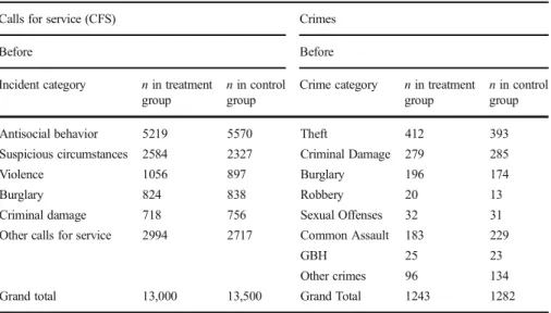
The total number of incidents in the hot spots, broken down into calls for service (CFS) and crime counts, before and during the experimental period, are shown in Table1. One

year before the experiment began, the hot spots attracted 26,500 calls-for-service and 2,525 crimes. The majority (72.89 %) of the calls fell into the top five incident categories: antisocial behavior (40.71 %), suspicious circumstances (18.53 %), violence (7.37 %), burglary of dwelling (6.27 %) and criminal damage (5.56 %). The leading crime types, at 94.81 % of all crimes, comprised the top five major crime categories: theft (31.88 %), violence against the person (24.63 %),5criminal damage (22.34 %), burglary (14.65 %) and robbery (1.31 %).

The distribution of events at baseline values suggests that while the minimum requirement for being a hot spot was set as 36 incidents in a 12-month period, the meannumber of CFS per hot spot at baseline period was 368.06 (SD = 252.39). The baseline frequency of calls per hot spot was asymmetrical (skewness = 1.291; SE = .283), with some eligible hot spots experiencing up to 619 incidents. The same pattern emerged for crime data, with the mean number of crimes per hot spot being 35.07 (SD = 24.54) at baseline, with a highly skewed distribution (1.263; SE = .283), ranging from 3 to 85 crimes. None of the pre-treatment between-groups comparisons were significant [t= .4521(70);p= .652 (CFS) andt= .4844(70),p= .630 (crime incidents)].

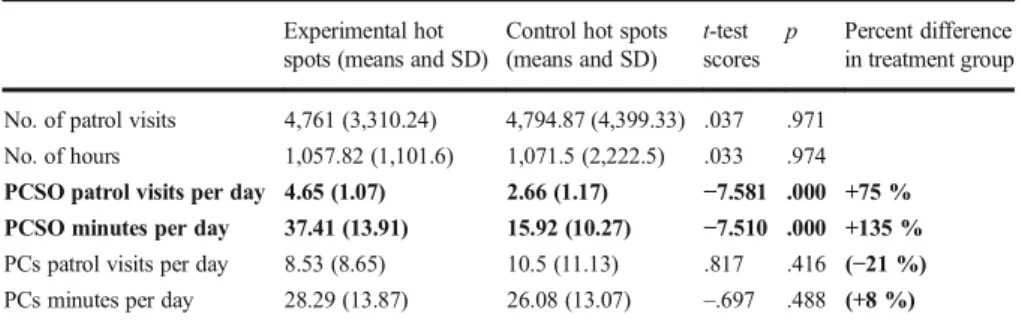
The GPS data for both PCSOs and Police Constables show high integrity in creating a big difference in PCSO patrol between treatment groups, while holding Police Constable patrol constant with no significant differences in PC measures between treatment groups (Table2). This finding applies to both measures of police activity: the duration of patrol time in the hot spots (measured in minutes), and the number of discrete patrol visits per day (see definition above), for the year of the RCT.

As shown in Table2, the treatment group hot spots received 135 % more PCSO patrol time than the control group hot spots: a mean of 37 minutes of PCSO patrol per day per treatment group hot spot versus about 16 minutes per day per hot spot in the

5

Common assault (the lowest category of assault, including slapping and pushing), grievous bodily harm, harassment, etc.

Table 1 Calls for service and crime data (baseline counts)

Calls for service (CFS) Crimes

Before Before

Incident category nin treatment group

nin control group

Crime category nin treatment group

nin control group

Antisocial behavior 5219 5570 Theft 412 393

Suspicious circumstances 2584 2327 Criminal Damage 279 285

Violence 1056 897 Burglary 196 174

Burglary 824 838 Robbery 20 13

Criminal damage 718 756 Sexual Offenses 32 31

Other calls for service 2994 2717 Common Assault 183 229

GBH 25 23

Other crimes 96 134

control group. The treatment group hot spots also received 75 % more PCSO visits per day, on average, relative to the control group hot spots.

These findings show far more clearly than any recent hot spot experiment the exact magnitude of the difference inBdosage^ measures of policing, as well as a means by which to estimate police compliance with the treatment program—which was substantial, but by no means perfect. While the PCSOs were tasked to provide 3 visits per day, for 45 minutes in total per day (that is, 15-minute patrols) in all hot spots, they delivered more visits, but fewer minutes, than required. In none of the comparisons of patrol minutes did the PCSOs deliver the treatment plan of 45 minutes per day, although they were only 18 % short of the goal (overall mean 37 minutes). In contrast, the number of visits exceeded the treatment plan by 57 %, with anBoverdose^of 4.7 patrol visits per hot spot per day.

The best news was that, while Police Constables made many more visits to the hot spots than did the PCSOs, there was minimal difference between treatment groups either in the minutes or visits delivered by PCs. TheseBfully weaponized^(for Britain) Police Constables spent on average 28 minutes per day per hot spot across all 72 of the hot spots, with double the number of visits per day (8.5) than the PCSOs. But as Table2shows, the 21 % fewer patrol visits PCs made in the treatment hot spots relative to controls (8.53 PC visits per day per treatment hot spot vs. 10.5 for controls) was not a significant difference (p= .416). Neither was the 8 % more PC patrol minutes (28.29 per hot spot per day) in the treatment group hot spots than in the controls (26.0 per hot spot per day) (p= .488).

By combining the measures of PCSO and PC activity, we can answer an additional research question: how much more policing did the treatment group have, overall, than the control group? For patrol minutes, we can report that the treatment group had a combined mean of PC and PCSO patrol time of 65.7 minutes per day per hot spot, compared to a combined mean total of 42.0 minutes at each control group hot spot. For patrol visits, the comparable figures are 13 visits per day per treatment group hot spot compared to 13.16 per spot for the controls. Thus, while our experiment created a 56 % increase in total patrol time in the treatment group relative to controls, it created what was essentially no difference in (or slightly fewer) patrol visits in the treatment group. These mean differences per hot spot create an interesting contrast to the pooled data across all treatment group hot spots. As reported in Table2, thetotalmean number of PCSO and PC patrols and thetotalmean PCSO and PC time spent in hot spots in the treatment and control conditions are nearly identical (4761 vs. 4794 patrol visits and 1058 vs. 1072 hours, respectively). This finding, along with the nonsignificant

Table 2 GPS data: means, standard deviations andttest scores Experimental hot

spots (means and SD)

Control hot spots (means and SD)

t-test scores

p Percent difference in treatment group No. of patrol visits 4,761 (3,310.24) 4,794.87 (4,399.33) .037 .971

No. of hours 1,057.82 (1,101.6) 1,071.5 (2,222.5) .033 .974 PCSO patrol visits per day 4.65 (1.07) 2.66 (1.17) −7.581 .000 +75 % PCSO minutes per day 37.41 (13.91) 15.92 (10.27) −7.510 .000 +135 % PCs patrol visits per day 8.53 (8.65) 10.5 (11.13) .817 .416 (−21 %) PCs minutes per day 28.29 (13.87) 26.08 (13.07) –.697 .488 (+8 %) Bold entries shows significant results detected in the treatment group

differences in terms of theBamount^of visibility of warranted police constables in the hot spots, suggests that should any treatment effect be observed, it is unlikely to be attributed tooverallcombination ofBhard^ andBsoft^ police presence, but rather to large differences between treatment groups inBsoft^policing delivered by the PCSOs. Main effects of soft policing

Table 3 lists the difference-in-differences in means (DID) for calls for service and crimes per hot spot, while comparing the pre-treatment and post-treatment figures for each hot spot. As shown, the crime DID for the 34 treatment hot spots was −5.85 (SD = 10.190) and for CFS the DID was−207.7 (SD = 166.598), while the crime DID for the 38 control hot spots was−3.55 (SD = 13.647) and for CFS the DID was−173.37 (SD = 158.046). These figures represent, for crimes, a 64.8 % greater reduction in crimes per hot spot in the treatment group relative to the controls,6with an absolute decline of 16.00 % in mean crimes per treatment hot spot relative to the absolute decline of 10.5 % crimes per control group hot spot. Had the treatment hot spots experienced a 10.5 % decline, they would have had 130 fewer crimes. Instead, the treatment group had 199 fewer crimes, or 68 fewer crimes than if they had generated the same reduction as in the control group or a mean of 2.6 more crimes prevented per hot spot. They also indicate a 19.79 % relatively greater mean reduction in CFS per treatment hot spot than the control group’s absolute percentage decline of 51.2 %, compared to a 61 % decline in the treatment group. Had there been a 51.2 % decline in the 34 treatment area baseline mean of 382 CFS per treatment group hot spot (the magnitude of the control group’s drop), it would have yielded a new mean of 186.4 CFS per hot spot. Instead, the treatment group mean was 174.7 per hot spot during the experimental year, a mean difference of 11.7 calls per hot spot, or 399 CFS prevented. As explained earlier, we converted these scores to standardized mean differences (Cohen’sd), in order to be able to compare our results to the existing body of literature. These results forBsoft^policing crime are highly comparable to the results forBhard^ policing. The effect size for reported crime data yields an effect size ofd=−.189 (95 % CI−.653, .27), and the effect size for calls for service isd=−.211 (95 % CI−.676, .252). These results mirror the overall treatment effect of hot spots policing found in Braga et al.’s (2012:58) systematic review (d=−.184).

Finally, we have counted nil reported incidents of assault or physical abuse against the PCSOs. Not one incident was identified in any of the crime reports or Calls for Service for the 72 hot spots during the 12 months of the experiment.

Measuring displacement

This section reports our analysis of displacement using the WDQ procedures described above. As Table3 shows, the target hot spots in the treatment group experienced a reduction during the experiment to 1044 generated crimes, from 1243 victim-generated crimes in the baseline year for agrosseffect (GE) in the treatment group of 199 fewer crimes. Theneteffect (NE), which takes into account the baseline period for

6

Calculated by first subtracting the treatment value from the control value, and the dividing the change by the control, multiplied by 100 to convert into percentages

Ta b le 3 Dif fer en ce -in -d if fe re n ce s in me an s (DI D) ca lls fo r se rvic e an d cr ime s (ba se lin e and pos t-r an dom as sig n me nt) : tr ea tm en t v er su s con tro l ho t sp o ts Contr o l hot spo ts T re at me nt hot spo ts 99 9 call s for ser vi ce Cr ime s 999 ca lls fo r ser vic e C rime s Hotsp o t P re -P os t-DID P re -P ost -DID H otsp ot Pr e-Post -D ID Pr e- Post-D ID 1 100 0 451 − 549 7 4 72 − 2 1 10 09 318 − 691 72 52 − 20 2 979 619 − 360 1 31 74 − 57 2 91 1 270 − 641 72 51 − 21 3 788 213 − 575 7 5 40 − 35 3 83 5 460 − 375 76 59 − 17 4 708 520 − 188 7 8 75 − 3 4 69 7 275 − 422 61 46 − 15 5 665 250 − 415 5 9 38 − 21 5 66 4 289 − 375 88 56 − 32 6 600 226 − 374 5 9 41 − 18 6 61 9 422 − 197 73 85 12 7 588 348 − 240 5 5 45 − 10 7 57 6 298 − 278 46 42 − 4 8 573 246 − 327 4 8 56 8 8 55 4 161 − 393 45 33 − 12 9 543 147 − 396 4 5 35 − 10 9 54 2 327 − 215 50 55 5 1 0 534 203 − 331 6 7 68 1 1 0 54 2 232 − 310 60 63 3 11 530 204 − 326 6 3 53 − 10 11 50 2 199 − 303 44 58 14 1 2 489 308 − 181 4 4 51 7 1 2 50 1 248 − 253 52 38 − 14 1 3 472 160 − 312 4 0 27 − 13 1 3 48 1 284 − 197 26 20 − 6 1 4 447 221 − 226 4 1 43 2 1 4 43 2 152 − 280 41 24 − 17 1 5 400 173 − 227 1 3 1 1 − 2 1 5 42 3 165 − 258 34 24 − 10 1 6 370 282 − 88 3 5 27 − 81 6 3 8 8 8 2 − 306 18 10 − 8 1 7 352 151 − 201 2 5 26 1 1 7 34 8 196 − 152 26 23 − 3 1 8 294 158 − 136 1 6 24 8 1 8 32 1 130 − 191 24 16 − 8 1 9 285 216 − 69 2 7 13 − 14 1 9 28 7 109 − 178 28 36 8 2 0 251 124 − 127 2 1 32 11 2 0 28 3 276 − 72 0 3 3 1 3 2 1 250 167 − 83 2 3 29 6 2 1 24 5 1 19 − 126 21 14 − 7

Ta b le 3 (c o n tin ue d) Contr o l hot spo ts T re at me nt hot spo ts 99 9 call s for ser vi ce Cr ime s 999 ca lls fo r ser vic e C rime s Hotsp o t P re -P os t-DID P re -P ost -DID H otsp ot Pr e-Post -D ID Pr e- Post-D ID 2 2 244 60 − 184 1 5 16 1 2 2 24 0 1 11 − 129 26 31 5 2 3 237 226 − 1 1 1 9 46 2 7 2 3 23 1 101 − 130 29 14 − 15 2 4 235 124 − 11 1 1 6 1 5 − 12 4 2 0 6 7 3 − 133 21 21 0 2 5 230 1 19 − 11 1 2 9 2 7 − 2 2 5 19 1 106 − 85 23 21 − 2 2 6 195 104 − 91 2 2 18 − 42 6 1 6 8 8 6 − 82 22 17 − 5 2 7 168 100 − 68 11 16 5 2 7 14 9 120 − 29 40 32 − 8 2 8 147 67 − 80 2 0 10 − 10 2 8 12 3 83 − 40 24 15 − 9 2 9 125 77 − 48 11 10 − 12 9 1 0 6 6 0 − 46 19 17 − 2 30 11 0 9 3 − 17 1 4 12 − 23 0 1 0 1 4 9 − 52 15 11 − 4 3 1 105 55 − 50 1 0 13 3 3 1 93 42 − 51 15 11 − 4 3 2 105 96 − 91 9 1 4 − 53 2 8 8 3 8 − 50 16 3 − 13 3 3 93 39 − 5 4 89 1 3 3 7 84 2 − 36 6 6 0 3 4 87 52 − 35 1 2 10 − 23 4 6 6 1 6 − 50 10 7 − 3 3 5 87 83 − 4 1 82 91 1 3 6 83 37 − 46 8 8 0 3 7 69 129 60 4 6 2 3 8 62 64 2 7 8 1 T O T A L 13, 500 6,91 2 − 6,58 8 1 ,282 1, 147 − 135 13 ,000 5,9 39 − 7, 061 1,243 1, 044 − 199 Me an − 173. 368 − 3. 553 − 207. 676 − 5. 853 SD 158 .046 1 3.647 1 66.596 10.19 0