Working Paper No. 13/2009 (23)
High-Frequency and Model-Free Volatility Estimators
(This work was supported by the Foundation for Polish Science)
Robert
Ś
lepaczuk
Faculty of Economic Sciences University of Warsaw
Grzegorz Zakrzewski
Credit Risk Management Expert Deutsche Bank PBC S.A. [address]
[e-
Abstract
This paper focuses on volatility of financial markets, which is one of the most important issues in finance, especially with regard to modeling high-frequency data. Risk management, asset pricing and option valuation techniques are the areas where the concept of volatility estimators (consistent, unbiased and the most efficient) is of crucial concern. Our intention was to find the best estimator of true volatility taking into account the latest investigations in finance literature. Basing on the methodology presented in Parkinson (1980), Garman and Klass (1980), Rogers and Satchell (1991), Yang and Zhang (2000), Andersen et al. (1997, 1998, 1999a, 199b), Hansen and Lunde (2005, 2006b) and Martens (2007), we computed the various model-free volatility estimators and compared them with classical volatility estimator, most often used in financial models. In order to reveal the information set hidden in high-frequency data, we utilized the concept of realized volatility and realized range. Calculating our estimator, we carefully focused on Δ (the interval used in calculation), n (the memory of the process) and q (scaling factor for scaled estimators). Our results
revealed that the appropriate selection of Δ and n plays a crucial role when we try to answer the question
concerning the estimator efficiency, as well as its accuracy. Having nine estimators of volatility, we found that for optimal n (measured in days) and Δ (in minutes) we obtain the most efficient estimator. Our findings confirmed that the best estimator should include information contained not only in closing prices but in the price range as well (range estimators). What is more important, we focused on the properties of the formula
itself, independently of the interval used, comparing the estimator with the same Δ, n and q parameter. We
observed that the formula of volatility estimator is not as important as the process of selection of the optimal
parameter n or Δ. Finally, we focused on the asymmetry between market turmoil and adjustments of
volatility. Next, we put stress on the implications of our results for well-known financial models which utilize classical volatility estimator as the main input variable.
Keywords:
financial market volatility, high-frequency financial data, realized volatility and correlation, volatility forecasting, microstructure bias, the opening jump effect, the bid-ask bounce, autocovariance bias,
daily patterns of volatility, emerging markets
1. Introduction
Almost everyone who works within financial markets, no matter if we mean their practical or theoretical aspects, is concerned about the volatility issue. The concept of volatility, especially predicting its future levels and managing the risk coming from its fluctuations, is of crucial importance for a number of reasons.1 The knowledge of true volatility is necessary when we compute all asset pricing models (CAPM, APT, multi-factor asset pricing models) and when we try to optimize mean-variance interrelation. It also has to be estimated in all kinds of VaR models including stress-testing and worst case scenarios, which try to predict the portfolio loss taking into account given significance level and the distribution of the returns. When we consider the option pricing techniques, volatility is the main input variable, the levels of which affect the final theoretical value the most, no matter which option valuation model we choose. Of course we cannot forget about implied volatility derived from option pricing models, which in practice is traded on the market instead of the value of the underlying contract; and the management of Vega, which is the most sophisticated issue when we consider the risk of actively managed option portfolio. Finally, we have to emphasize the management of portfolios of derivatives (futures, options or swaps), where what matters is not only the direction of the market but also, and most of all, an accurate prediction of future volatility (especially in the case of volatile market with high unexpected jumps between close and open), which is even more important for proper portfolio risk management. We should add here that volatility risk, highly correlated with liquidity risk, especially in the time of market turmoils, is nowadays the main source of risk in financial system, where the hedge funds managing billions of dollars use the financial leverage in almost each trade. This subject is particurarly important in the globalized financial markets, where significant turmoils happen more often (May-June 2006, March, August, November 2007 or January 2008) and, what is more important, spread all over the world with ultra-fast speed. Therefore, the observation of modern capital markets prompts us to design the research that pays crucial attention to the ways of risk quantifying.
Contemporary state-of–the–art is that the classical volatility estimator (standard deviation of daily log returns) or implied volatility (used in option modelling) are the measures of volatility most often used in models, whenever we need the true measure of volatility. However, as the latest research revealed (Andersen et al. (2001), Yang and Zhang (2000), Shu and Zhang (2006), Martens and Dijk (2007)) we can find other, more efficient and yet unbiased estimators of true volatility. Among other things, we want to verify this notion in our paper.
Taking into consideration all the above-mentioned issues and trying to find better estimators of true volatility by studying the properties and merits of realized range2 and realized volatility3, we calculated the following measures of volatility:
1. classical volatility estimator (a n n u a l_std
SD
n) 2. realized volatility (a n n u a l_stdRV
n)3. realized range (a n n u a l_std
RR
n)1 Investors who did not consider these issues as key factors were taught a very expensive and painful lesson. One
of numerous examples is the collapse of prestigious Long Term Capital Management in 1998, which almost destabilized global financial system (Lowenstein, 2000).
2 The measure of daily volatility computed by summing high-low ranges for intra-day intervals. 3 The measure of daily volatility computed by summing squared returns for intra-day intervals.
4. Garman-Klass volatility estimator (a n n u a l_std
GK
n) 5. Rogers-Satchell volatility estimator (a n n u a lstd nRS
_ )
6. Yang-Zhang volatility estimator (a n n u a l_std
YZ
n)7. realized volatility with autocovariance correction ( annualstd n
RV
AC
_
1 )
8. scaled realized volatility (a n n u a l_stdq
RV
n) 9. scaled realized range (a n n u a l_stdqRRn)After obtaining given estimators of volatility, we compared their distribution with the classical volatility estimator to find out all the details concerning the information content of each of them and specify the main differences between them. Next, we focused on several aspects concerning the way of its measuring, i.e.: number of days for scaling factor (q=?), the optimal sampling frequency (Δ=?), and the length of the memory (n=?), so as to ensure the extraction of appropriate information from todays and previous quotations. The detailed discussion of parameter n constitutes the important contribution of our paper to volatility literature. Much as the issue is often omitted, we show it to play a crucial role in the performance of volatility estimators, stability of fluctuations of annualized and averaged estimators and the set of information incorporated in their calculation formula.
We noticed the necessity of using high, low, open and close prices instead of only close prices in the process of estimation. It is clearly observed that a substantial part of daily volatility can be revealed only when we base our calculations on the intraday range, revealing its intra-interval fluctuations, as well (Slepaczuk and Zakrzewski, 2008). Not including this information in the close-to-close estimators was the reason, while we added the various concepts of realized range estimators to our comparison (RR, GK, RS, YZ, etc.).
One of our main goals was to find the most efficient estimator, which would take us closer to the true volatility estimator. In order to accomplish this goal, we calculated several statistics describing relative performance of our volatility estimators (the variance efficiency ratio, the modified variance efficiency ratio, and the relative variance efficiency ratio). We also discussed the issue of accuracy, however, we leave the detailed investigation of that subject for the future research.
The consecutive idea of this paper was to show that computing volatility on high-frequency data could provide us with valuable information about fluctuations of the market which is not revealed in the data on the daily basis, especially when the market is volatile during the day. That was the reason for calculating our estimators on various sampling frequencies (from 5-minute to daily interval).
Finally, we have to stress that the main objective of this work, which was to find the best estimator of true volatility, was only the step into further investigations, which concern forecasting future volatility levels. What we have to do first in the process of selecting the best econometric models for forecasting is to choose the most appropriate input data (one of the proposed volatility estimators) which significantly influence accurate volatility forecasts.
Taking into account all the above mentioned, we formulated several hypotheses, which will be verified further in this paper:
1. Computing volatility on high-frequency data will provide us with valuable information about fluctuations of the market, which is not revealed in the data on the daily basis. It is
indirectly connected with greater efficiency of estimators calculated on the basis of HF data.
2. During the estimation process we should utilize information included in price range (high, low, open and close prices), in order to obtain the most efficient estimators.
3. The efficiency of volatility estimator is closely connected with the length of the memory (parameter n) used in the process of calculation.
4. The efficiency of the estimator concerning its formula is only revealed when compared to the other estimator calculated on the basis of the same interval delta and parameter n. 5. Various concepts of volatility estimators could over or under-estimate the actual level of volatility depending on their calculation formula.
To accomplish described goals we planned the structure of our paper as follows. Next section describes the recent literature and some stylized facts about volatility. Theoretical background, formulas and the overall context of presented research are in the third part. Fourth section contains the description of data used in the process of analysis. The process of selection of q, Δ and n is described in the fifth section. The consecutive part contains the comparison of distributions of volatility estimators. The seventh part focuses on the connection between market turmoil and the behaviour of different volatility estimators. In this section we also describe implications of the results for financial models. The last section concludes and defines paths for further researches.
2. Literature review
The concept of volatility estimators is widely researched in financial literature. Scientists try to find the best estimator of true volatility, which is not observed/rather latent process, through numerous researches on daily, weekly or high frequency financial data.
Contemporarily, the most frequently used estimator is still classical volatility estimator (the sum of squared differences of ith return and the mean return over the analyzed period of
time) which is the part of many kinds of financial models (Black-Scholes model, CAPM, APT, input variable in various GARCH and ARCH models, as well as stochastic volatility models, etc.) and which is frequently treated as sufficient estimator of true volatility process. Although this estimation is to a large extend successful, we are aware of the fact that it is possible to find better, more efficient, still unbiased and consistent estimators. The most important disadvantage of SD is that it is calculated on the daily basis, not revealing intraday fluctuations and that it is supposed to have low efficiency in comparison with other volatility estimators (e.g. Martens and Dijk, 2007, Yang and Zhang, 2000, Shu and Zhang, 2006).
Since the concept of volatility has grown in importance through the last forty years, many new concepts of volatility estimators focused on gaining on efficiency and being robust to all existing microstructure biases (bid-ask spread, the opening jump effect, non-trading bounce, etc.) have been invented. Therefore we have thoroughly and chronologically studied the most influential works concerning the issue of volatility estimators and their properties, in order to place our research as the natural consequence of the contemporary state-of-the-art and focus on the most important details which were not sufficiently explained in the previous works.
Merton (1980), who was the first to propose realized volatility concept (the sum of squared returns over the analyzed period of time measured in equidistant periods) as the unbiased and consistent estimator of daily variance 2
t
on condition that the returns have a zero mean and are uncorrelated. He agreed that RV is the true volatility estimator when
returns are sampled as often as possible. This concept was later heavily researched by Taylor and Xu (1997) and Andersen et al. (1998, 2000, 2001a and 2001b) as well as others, who additionally paid close attention to microstructure bias which unfortunately grows in importance as the sampling frequency increases.
In 1980, Parkinson introduced the new concept, which utilized price range (high price - low price, or consequently their logs) in order to reveal all the information set included in the price fluctuations. This improvement led to range-based volatility estimator which was still unbiased if the mean was equal zero and almost 5 times more efficient than the classical volatility estimator.
Next concept of Garman and Klass (1980) improved Parkinson’s estimation by including not only high and low prices but open and close prices, as well. They defined the minimum-variance unbiased estimator for Brownian motion with zero-drift. Moreover, they proved that their range based volatility estimator is eight time more efficient than the classical volatility estimator.
Following the discoveries described above, Rogers and Satchell (1991) proposed a new approach to volatility estimation. Suggested concept was unbiased and independent of the drift term. Their estimator improved the main drawback of Garman-Klass estimator which was biased if used in the case of non-zero drift. However, Rogers-Satchell estimator still assumed no opening jump effect and was unbiased only under this assumption.
The next step into increasing volatility literature, where successive researchers attempted to find the unbiased estimators, which would be independent of both opening jump and the drift term, was Yang and Zhang (2000) with their multiperiod volatility estimator based on high, low, open and close prices. The Yang-Zhang estimator had the following properties: (a) unbiased, (b) independent of the drift, (c) consistent in dealing with the opening jump and (d) smallest variance among all the estimators with similar properties (the typical biweekly Yang-Zhang variance estimation was over 7 times more efficient than the classical variance estimator).
Andersen and Bollerslev started to popularize the notion of realized volatility and correlation in 90s having written the numerous research papers (Andersen and Bollerslev, 1998, 1999a, 1999b) devoted to the techniques focusing on many possible aspects and dimensions of that issue, especially the properties of such estimator calculated on the high frequency data. They noticed that the realized volatility is a more efficient and unbiased estimator of volatility than the popular daily classical volatility estimator. Moreover, it converges to the true underlying integrated variance when the length of the intraday interval goes to zero (Andersen et al. 2001a, 2001b). They found that the efficiency of the daily high-low range is between that of the realized variance computed using 3- and 6- hour returns. Estimating realized volatility of stock returns they noticed that the sampling frequency of 5- and 30-minute intervals strike a balance between the increasing accuracy of higher frequencies and the adverse effects of market microstructure frictions (Andersen et al., 2001a, 2003).
The discussion of the volatility estimation techniques was enriched by the description of distribution of volatility during the normal stock session which we can name daily patterns of volatility (Taylor and Areal, 2000). Basing on five-minute returns they presented the distribution of the volatility of FTSE-100 index focusing on significant jumps of volatility during the day, caused by the announcement of US or UK macro data. They also revealed that the patterns of volatility are considerably diverse through consecutive days of the week. Studying the distribution of the logarithm of volatility and that of returns standardized by realized volatility they confirmed that it is almost exactly normal.
Zhang et al. (2005) went one step further and developed the estimator which combined realized variance estimator obtained from returns sampled at two different frequencies. The realized variance estimator obtained using a certain (low) frequency was corrected for bias due to microstructure noise using the realized variance obtained with the highest available sampling frequency.
Ait-Sahalia et al. (2005) and Hansen and Lunde (2006b) revealed that returns at very high frequencies are distorted such that the realized variance becomes biased and inconsistent. Deriving the theoretical properties for realized range in a world with no market microstructure noise and with continuous trading, Christensen and Podolskij (2005) stated that this estimator is five times more efficient than the realized variance sampled with the same frequency and converges to the integrated variance with the same rate.
When testing the relative performance of various historical volatility estimators that incorporate daily trading range Shu and Zhang (2006) found that the range estimators perform very well when asset price follows a continuous geometric Brownian motion. However, significant differences among various range estimators are detected if the asset return distribution involves an opening jump or large drift. Nonetheless, the empirical result is supportive of the use of range estimators in estimating historical volatility.
Martens and Dijk (2007) tried to develop the concept of realized range by introducing scaled realized range which was additionally robust to microstructure noise. They noticed that realized range with their bias-adjustment procedure was more efficient than realized variance when using the same sampling frequency.
Discussing the issue of volatility estimators we cannot forget about implied volatility derived from the market prices of options with help of adequate theoretical model. The concept, which has been developing successfully from the mid 70s, got the inspiring injection of new theoretical thought after publication of Derman et al. (1999), who explain the properties and the theory of both variance and volatility swaps, deriving volatility directly from option prices basing on model-free and non-parametric approach to volatility estimation. They also design the framework for hedging Vega, showing how a variance swap can be theoretically replicated by a hedged portfolio of the strip of out of the money options (Call and Put) with adequate weights. Assuming that the fair value of the variance swap is the cost of the replicating portfolio, they derive analytic formulas for theoretical fair value in the presence of realistic volatility skew. Nowadays, the above concept lies behind the theoretical formulas designed for VIX and many other volatility indexes (VXO, VXN, VDAX, VDAX-NEW, VSMI, and recently computed VIW204). Moreover, VIX index is even the basis instrument, for derivatives (futures and options) quoted on the CBOE and this issue will be important in the discussion presented in the sections seven and eight.
Before we go to the main part of this paper let us look at some stylized facts established between theoreticians and practitioners dealing with the issue of volatility:
Volatility time series are mean-reverting; Moreover, analyzing the behaviour of VIX we can even say that it is “minimum reverting process” (Slepaczuk and Zakrzewski, 2007). Long memory phenomenon or the persistence effect in the volatility time-series, i.e. after negative or positive shock in volatility, the shock dies out very slowly (Baillie et al., 1999 – fractionally integrated time series).
4 VIW20 is the volatility index for WIG20 index, the main equity index for the Polish stock market (Slepaczuk and
Volatility clustering, i.e. we observe distinct periods when volatility clusters on the high or low level for the long period of time (Andersen et al., 2001a). This effect is closely related to long memory effect, described above.
The leverage effect revealing asymmetric volatility reaction on the shocks in the basis stock market index, i.e. sudden jumps of volatility connected with the sharp downward movement and moderate increase or even decrease in the time of upward movement (Black, 1976; Ebens, 1999; Andersen et al., 2001a). Additionally, Andersen et al. (2001a) showed that this effect is stronger on the aggregated level (market stock indexes) than for individual stocks.
Strong negative correlation with the basis index, which additionally strengthens in the time of market turmoils, contrary to the correlation between normal instruments (stocks, bonds, etc) where initially defined negative correlation disappears when the market is on the edge of crash (Slepaczuk and Zakrzewski, 2007).
Volatility is time varying and predictable to a certain extent (Giot and Laurent (2004) and Martens and Dijk (2007),
The distribution of variance is characterized by high kurtosis, positive skewness and non-normality, but the logarithm of volatility (realized volatility) is approximately normal (Giot and Laurent (2004), Andersen et al. (2001a and 2001b).
Volatility-in-correlation effect, the strong positive relations between individual stock volatilities and the corresponding strong positive relations between contemporaneous stock correlations (Andersen et al., 2001a). There is a systematic tendency for the variances to move together and for the correlations among the different stocks to be high/low when the variances for the underlying stocks are high/low, and when the correlations among the other stocks are also high/low.
Upward and downward sloping term structure of volatility, especially when we consider implied volatility, which can be easily explained by the mean reverting process. When the short-term implied volatility is relatively high/low then the term structure is downward/upward sloping.
While conducting our research we will compare our results with stylized facts mentioned above.
3. Theoretical background, and the notion behind each formula
On the ground of presented literature we assumed that volatility estimators calculated on the basis of high-frequency data including information about intraday range should be the most efficient ones. Choosing the set of estimator for our research we took this notion into account.
The definitions of our estimators are presented below. First, we present the formula to calculate classical volatility estimator (standard deviation of log returns) which gives us, the average variance over the period of n-days:
) 1 ( ) ( 1 ) * ( 1 1 1 2 ,
n t N i t i n r r n N VAR where: nVOL – variance of log returns calculated on high frequency data on the basis of last n-days,
t i
r
, – log return for ith interval on day t with sampling frequency equal Δ, which iscalculated in the following way:
) 2 ( log log , 1, ,t it i t i C C r t i
C, – close price for ith interval on day t with sampling frequency equal Δ,
r – average of log returns for ith interval on the basis of last n-days with sampling
frequency equal Δ, which is calculated in the following way:
)
3
(
*
1
1 1 ,
n t N i t ir
n
N
r
NΔ – the amount of Δ intervals during the stock market session,
n – the memory of the process measured in days, used in the calculation of adequate estimators and averages.
One of the first estimators which we choose in our study is the Parkinson estimator (Parkinson, 1980). Initially it was calculated on the basis of daily intervals, but after Martens and Dijk (2007) we decided to use intraday prices, in order to obtain so called realized range. We aggregate high-low ranges for intraday intervals to obtain daily realized range:
)
4
(
2
log
4
)
(
1 2 , , ,
N i t i t i tl
h
RR
where: tRR
, – daily realized range calculated for day t with sampling frequency equal Δ, ti
l
, – log of minimum price (log
L
i,t) for ith interval on day t with sampling frequencyequal Δ,
t i
h
, – log of maximum price (log
H
i,t) for ith interval on day t with samplingfrequency equal Δ,
Next, after Andersen et al. (2001), Taylor and Areal (2000) and Martens and Dijk (2007) we shortly explain the theoretical background behind the concept of realized volatility estimator. Realized volatility computed from high-frequency intraday data is an effective error-free and model-free volatility measure, considering that we choose the optimal sampling frequency. Furthermore, construction of realized volatility is trivial as one simply sums intra-period high-frequency squared log returns (or cross products, for realized covariance5), period by period. For example, for a 7-hour market (420 minutes), daily realized volatility based on Δ-minute underlying returns is defined as the sum of the NΔ
intra-day squared Δ-minute returns, taken day by day6:
) 5 ( 2 1 1 , 1 , 2 , ,
N i N i t i j N i j t j t i t r r r RVwhere Ci,t denotes the close price of ith interval on day t and ri,t denotes the log-return of ith
interval on day t. Assuming that the returns have zero mean and are uncorrelated, and following the discoveries of Andersen, Bollerslev, Diebold and Labys (2001), we can treat
5
Having known the big importance of the correlation of returns we decided to leave this subject for consideration in forthcoming papers.
N i t ir
1 2, as consistent and unbiased estimator of daily variance 2 t
and formula for daily realized volatility becomes simpler:)
6
(
1 2 , ,
N i t i tr
RV
The Garman-Klass volatility estimator (Garman-Klass, 1980) which utilizes the open and close price in addition to the high and low prices is calculated as:
0.5*( ) (2*lo g2 1)*
(7) 1 2 , 2 , ,
N i t i t i t i l r h GKNext, we calculated Rogers-Satchell volatility estimator (Rogers and Satchell, 1991):
( )*( ) ( )*( )
(8) 1 , , , , , , , ,
N i t i t i t i t i t i t i t i t i o h c l o l c h RS where: t io
, – log of open price (log
O
i,t) for ith interval on day t with sampling frequency equal Δ,t i
c
, – log of maximum price (log
C
i,t) for ith interval on day t with samplingfrequency equal Δ,
Consecutive estimator, presented by Yang and Zhang (2000) improved the most important imperfections connected with the previous ones. The formula for Yang-Zhang volatility estimator is as follows:
)
9
(
)
1
(
n c o nRS
k
kV
V
YZ
where: ) 10 ( * 1 , log log , ) ( 1 ) * ( 1 1 1 , , 1 , , 1 1 2 ,
n t N i t i t i t i t i n t N i t i o o n N ro C O ro ro ro n N V ) 11 ( * 1 , log log , ) ( 1 ) * ( 1 1 1 , , , , 1 1 2 ,
n t N i t i t i t i t i n t N i t i c rc n N rc O C rc rc rc n N Vand the constant k chosen to minimize the variance of this estimator is given by:
) 12 ( 1 * 1 * 34 . 1 34 . 0 N n N n k
Alternate formula for volatility estimator was presented in Hansen and Lunde (2006b). Their kernel-based estimator tried to remove the bid-ask bounce by adding autocovariances to the realized variance. In our research we included n
AC1RV , which incorporates the
first-order autocovariance:
)
13
(
2
2 , 1 , 1 2 , 1
N i t i t i N i t i ACRV
r
r
r
Two last estimators which were taken into account in our study were the concepts of scaled realized range and scaled realized volatility proposed by Martens and Dijk (2007). They suggested a bias correcting procedure based on scaling the realized range/volatility
with the ratio of the average level of daily range/volatility and the average level of the realized range/volatility over the q previous days:
) 14 ( , 1 , 1 , t q a a t q a a t daily q RV RV RV RV
) 15 ( , 1 , 1 , t q a a t q a a t daily n q RR RR RR RR
where: tRV
, - daily realized volatility calculated for day t with sampling frequency equal Δ,a t d a ily
RV
,-
daily realized volatility calculated for day t based on daily data,t
RR
, - daily realized range calculated for day t with sampling frequency equalΔ, a
t d a ily
RR
,-
daily realized range calculated for day t based on daily data,The process of scaling was based upon the idea that daily realized range is (almost) uncontaminated by microstructure noise, and thus provides a good indication of the true level of volatility. While implementing this bias adjustment we have to choose the proper number of trading days q used to compute the scaling factor. Martens and Dijk (2007) suggest that if the trading intensity and the spread do not change for the asset under consideration, q may be set as large as possible to gain accuracy. Naturally, in practice both features tend to vary over time, which suggests that only the recent price history should be used and q should not be set too large. When we consider the data for WIG20 index futures utilized in our research, we see that the spread is relatively small (1 point), but the trading intensity varies significantly over time. This variation in the average spread suggests that the ratio of the average level of the daily realized range relative to the average level of realized range changes over time. Therefore, we decided to compute the scaling factor using the previous q trading days, where q was equal: q= {5, 10, 15, 21, 42, 63, 84, 105, and 126}. Then we choose the most appropriate scaling factor on the base of the estimator efficiency.
Looking at the formulas presented, we can distinguish multi- and one-period estimators, computed in many different ways, thus in the next step we implement two different methods of averaging. Next, we will annualize these estimators assuming that there is 252 working days in a year and we will take the square root of our estimator to obtain standard deviation as a measure of volatility instead of variance.
)
16
(
*
*
252
_s td n n annualSD
N
VAR
)
17
(
*
*
252
_s td n n annualYZ
N
YZ
)
18
(
]
_
[
1
252
]
_
[
1 , _
n t t n s td annualest
vol
n
est
vol
where:
]
_
[
vol
est
- RR, RV, GK, RS,AC1RV
,qRV
,qRR
, n std annualest
vol
_
]
[
_ - annualized volatility estimator: a n n u a lstd n
RR
_ , a n n u a l_stdRV
n, n std a n n u a lGK
_ ,a n n u a l_stdRS
n, n std annual ACRV
_ 1 . n std a n n u a l qRV
_ ,a n n u a l_stdqRV
n,Naturally, everywhere we use log we mean natural logarithm. After the presentation of all the formulas for volatility estimators we come to the point of choosing the most adequate n, Δ, and q in order to select the best estimator of true volatility (section six). However, let us describe our data sets first.
4. Data and descriptive statistics
Our empirical analysis is based on high-frequency financial data for WIG20 index futures7. WIG20 consists of 20 largest companies quoted on WSE and is computed as a weighted measure of the prices of its components. The 5-minute data, supplied by Information Products Section from WSE8, cover the period from June 2, 2003 to July 7, 2007. The number of 5-minute returns for a trading day depends on the trading hours for futures contracts but this have been changed once during our research period. The trading took place from 9:00 a.m. to 4:00 p.m. for the time period from June 2, 2003 until September 30, 2005 and from 9:00 until 4:30 p.m. 9 for the next two years from October 3, 2005 until July 7, 2007. Thus, we had 84 or 90 five-minute returns for a day in the research period, but in order to conveniently define delta-minute returns, we removed all prices recorded after 4:00 p.m., and as a result we were left with 84 five-minute returns during the day.10 All returns were computed as the first difference in the regularly time-spaced log prices of WIG20 index futures, with the overnight return included in the first intraday return. After correction for outliers (three on the basis of five-minute intervals and two on the daily basis) we get a total of 1031 trading days and a total of 86414 five-minute intervals. The intraday intervals for different delta (taking daily prices into consideration as well) were obtained from the basic five-minute data set.
Table 4.1 summarizes the descriptive statistics for five-minute data interval divided into two subsets: the original data (returns-I) and the data after modification (returns-II) described above. We include this comparison in order to show that our modification does not significantly change the properties of the data set used in our research. Analyzing both returns, we can see high kurtosis and negative, but small skewness. The average returns are small and are not significantly different from zero. The distribution of the returns is
7
We based our study on the continuous time series for futures, where expiring futures contract was replaced by the next series, where the number of open positions achieved the higher value. Described mechanism is one of the most common ways of creating continuous time series for futures. We do not have enough data for the longer period of time because of the short time to expiration of individual future contract, for that reason we had to create continuous futures index.
8 Warsaw Stock Exchange.
9 In practice, the continuous trading finished at 4:10 p.m., then the close price was settled between 4:10 p.m. and
4:20 p.m., and next investors could trade until 4:30 p.m. only on the basis of close price. Therefore, we could say that we have 86 instead of 90 intervals in the second period.
10 We adjusted high, low and close price in the last 5-minute interval (from 3:55 p.m. to 4:00 p.m.) with the
information included in the intervals from 4:00 p.m. to 4:10 p.m. and the daily close price. Table 4.1 presents the descriptive statistics for our data set (five-minute returns) with and without this restriction as to confirm that this transformation did not influence its properties.
leptokurtic, i.e. it is almost symmetric and has fat tails and a substantial peak at zero. Testing for normality we get the same results for both data sets, i.e. the statistics reveal non-normality of the data sets tested. The most important is that the descriptive statistics for both data sets do not differ significantly, which allows us to use modified data set (returns-II) in the research.
Table 4.1. The descriptive statistics for log returns of analyzed index futures returns for the period from June 2, 2003 to July 7, 2007.a
returns-I b returns-II c
N 86414 84818
Mean 0.000013534 0.000012834
Median 0 0
Variance 2.3131977E-6 2.3085858E-6
Std Dev 0.0015209 0.0015194 Minimum -0.0305313 -0.0305313 Maximum 0.0279413 0.0279413 Kurtosis 24.2092143 23.9819602 Skewness -0.1556275 -0.1774762 P1 -0.0041335 -0.0041140 P5 -0.0021031 -0.0021224 P10 -0.0014276 -0.0014461 P90 0.0014535 0.0014724 P95 0.0021146 0.0021330 P99 0.0042061 0.0041754
Test for Normality
Kolmogorov-Smirnov Statistic 0.105333 0.105758
p-value <0.0100 <0.0100
Cramer-von Mises Statistic 379.7725 356.5796
p-value <0.0050 <0.0050
Anderson-Darling Statistic 2122.372 1988.245
p-value <0.0050 <0.0050
a The table contains the descriptive statistics for five-minute returns for original data and the data with prices
recorded between 9:00 and 16:00 only. The statistics presented above are: number of observation, mean, median, variance, standard deviation, minimum, maximum, kurtosis, skewness and normality tests. b the original data. c the
modified data with prices recorded between 9:00 and 16:00 only.
Following the discoveries of Ait-Sahalia et al. (2005) we wanted to answer the question if we really need the data sampled as often as possible or 5-, 10-, 15- or even 30-minute intervals are enough. Therefore, we tried to choose the optimal sampling frequency (Δ
parameter), i.e. the best interval when we consider maximizing the efficiency and minimizing the microstructure bias (bid-ask bounce and infrequent trading bias) combined with autocovariance bias. Areal and Taylor (2000) agreed that five-minute returns are the highest that avoid distortions from microstructure effect such as bid-ask bounce. On the other hand, Oomen (2001) suggests that the use of equally-spaced thirty-minute returns strikes satisfactory balance between the accuracy of the continuous-record and the market microstructure frictions. We wanted to answer the same question on the basis of the data being researched. Finally, we decided to choose a range of sampling frequencies in the process of calculating the various volatility estimators and leave the moment of selecting it for the next section, where we focus on the efficiency of the estimator.
The point of our interest in the next sections will be to find the most efficient estimator with regard to the estimation parameters: q, n and delta. In the process of calculation we used delta which are divisors of 420 (the number of minutes during the normal stock market session), i.e. delta = {5, 10, 15, 30, 60, 105, 210, 420}. As for the memory parameter (n) and the scaling factor for scaled estimator (q) we establish our set of possibilities basing on the time intervals, i.e. equivalent of one day, week, month, etc., naturally taking into account only working days. Therefore, we calculated volatility estimators for the following parameters: n = {1, 5, 10, 15, 21, 42, 63, and 126} and q = {5, 10, 15, 21, 42, 63, 84, 105, and 126}.
5. The optimal sampling selection and the length of the memory of the process. In order to solve the problem of optimal sampling selection, we had to calculate the volatility estimators for all values of q, n, and delta parameters. Given that we used 9 different possible values of q and 8 different possible values of n and delta, in result we got a quite substantial number of combinations for each volatility estimator:
1. 64 possible values for:a n n u a l_std
RR
n, a n n u a l_stdRV
n, a n n u a l_stdGK
n,n std a n n u a l
RS
_ , n std annual ACRV
_ 1 , n std a n n u a lYZ
_ , a n n u a lstd nSD
_, which depend on n and delta parameters (8x8 possibilities).
2. 576 possible values for scaled estimators: a n n u a l_stdq
RR
n,a n n u a lstd n qRV
_, which depend on n, q and delta parameters (8x9x8 possibilities),
which totaled in 1600 volatility estimators.
Having calculated these estimators, we had to choose the adequate methodology for measuring the efficiency of the estimator. We agreed with Yang and Zhang (2000) that the variance/standard deviation of an estimator measures the uncertainty of the estimation, i.e. the smaller the variance/standard deviation, the more efficient the estimation. They concluded that, from the point of view of both theoretical consideration and practical application, it is desirable to find the minimum variance/standard deviation unbiased estimator. Garman and Klass (1980) who defined the efficiency of a variance estimator to be the ratio of the variance of the classical daily volatility estimator to that of current estimator, claimed that the higher the ratio, the more efficient the estimator for a given number of periods. Primal formula for variance efficiency ratio was:
) 19 ( ) ] ([var_ ) ( n n daily est Var VAR Var Eff where:
Eff - variance efficiency ratio,
) (VARd a ilyn
Var - variance of the classical variance estimator,
)
]
([var_
est
nVar
- variance of the specific variance estimator,The puzzling thing in the above formula was that it compared the estimators calculated on the basis of different intervals (delta parameter) and various price histories (parameter n), what could be misunderstandable in the process of parameters selection. When we use different n or delta, as a result we do not get the most efficient estimator with regard to its formula but the outcome efficiency is conditional on parameter n and parameter delta. We
tried to avoid this imperfection while estimating the efficiency of our estimators. Therefore, basing on the definition of Garman and Klass we define new indicator: modified volatility efficiency ratio (mEff) as the ratio of standard deviation of annualized SD (calculated on the basis of specific interval delta for the last n days) to the standard deviation of the specific volatility estimator (calculated on the basis of the same delta and n parameters):
) 20 ( ) ] _ [ ( ) ( _ _ n s td annual n s td annual est vol std SD std mEff where:
mEff - modified volatility efficiency ratio,
)
(
annual_stdSD
nstd
- standard deviation of annualized classical volatility estimator,)
]
_
[
(
annual_s tdvol
est
nstd
- standard deviation of annualized volatility estimator,We utilized mEff to choose the optimal parameter q, with regard to the efficiency of scaled estimators (table 5.1-5.2 and figure 5.1-5.2 contained the results for RR and table 5.3-5.4 and figure 5.3-5.4 present the results for RV). Unfortunately, the construction of mEff makes it relatively difficult to compare our estimators with respect to different delta and n, independently of their absolute values. Therefore, we decided to calculate the relative volatility efficiency ratio (rEff) where numerator and denominator were divided by mean of adequate volatility estimator in order to correct imperfection mentioned above. We used rEff in the process of choosing the optimal frequency delta and the most appropriate price history (parameter n). Naturally, line of reasoning remained the same. The higher ratio indicated the more efficient the estimator.
)
21
(
)
]
_
[
(
)
]
_
[
(
/
)
(
)
(
_ _ _ _ n s td annual n s td annual n s td annual n s td annualest
vol
mean
est
vol
std
SD
mean
SD
std
rEff
where:rEff - relative volatility efficiency ratio,
) (annual_stdSDn
mean - mean of annualized classical volatility estimator,
) ] _ [
(annual_s td vol estn
mean - mean of annualized classical volatility estimator,
We were not able to present the results for all possible combinations of delta parameter, so we chose delta equal 5- and 30-minute interval, as the ones most often chosen in the literature. As for the lack of free place we present here only the results for two deltas but all the remaining lead us to the same conclusion concerning the selection of q. The figures 5.1-5.2 and tables 5.1-5.1-5.2 present the results for scaled RR with delta equal 5 and 30 minute for all n and all q.
The efficiency ratios for volatility estimators presented in this section were calculated for the period from June 3, 2004 to July 7, 2007. We have to leave 252 daily data (from June 3, 2003 to July 7, 2007) because such amount is required to calculate the first value of
126 _ 126RR std annual and _ 126 126RV std
annual (126 daily data for scaled parameter and 126 in the process of averaging and annualizing).
Table 5.1. The modified volatility efficiency ratio (mEff) for a n n u a lstdq
RR
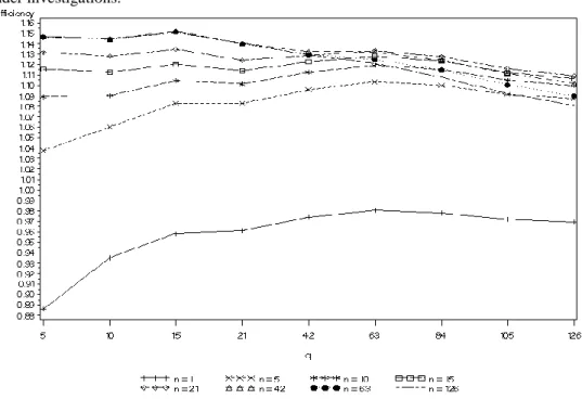
5n _ for all n under investigations.a n 1 5 10 15 21 42 63 126 q 5 0.886 1.038 1.089 1.116 1.132 1.146 1.146 1.147 10 0.935 1.060 1.090 1.113 1.128 1.144 1.144 1.145 15 0.958 1.083 1.105 1.120 1.135 1.152 1.151 1.151 21 0.961 1.083 1.102 1.114 1.124 1.140 1.140 1.140 42 0.974 1.096 1.113 1.123 1.129 1.132 1.130 1.129 63 0.981 1.104 1.119 1.128 1.133 1.132 1.125 1.121 84 0.978 1.100 1.115 1.123 1.128 1.124 1.115 1.108 105 0.972 1.091 1.105 1.112 1.116 1.111 1.101 1.092 126 0.969 1.087 1.100 1.106 1.109 1.102 1.090 1.081 a scaled RR is computed according to formula (18) for the data covering all period under investigation (from June2, 2003 to July 7, 2007) for delta = 5-minute interval.
Figure 5.1. The modified volatility efficiency ratio (mEff) for a n n u a l_stdq
RR
5n for all n under investigations.aa scaled RR is computed according to formula (18) for the data covering all period under investigation (from June
Figure 5.2. The modified volatility efficiency ratio (mEff) for a n n u a lstdq
RR
3 0n _for all n under investigations. a
a scaled RR is computed according to formula (18) for the data covering all period under investigation (from June
2, 2003 to July 7, 2007) for 30-minute interval.
Table 5.2. The modified volatility efficiency ratio (mEff) for a n n u a lstdq
RR
3 0n _ for all n under investigations. a n 1 5 10 15 21 42 63 126 q 5 1.001 1.115 1.161 1.185 1.197 1.208 1.206 1.210 10 1.051 1.141 1.168 1.189 1.201 1.214 1.211 1.215 15 1.072 1.162 1.182 1.197 1.208 1.223 1.220 1.222 21 1.076 1.162 1.180 1.193 1.201 1.214 1.211 1.213 42 1.088 1.176 1.192 1.202 1.207 1.211 1.206 1.207 63 1.092 1.180 1.194 1.204 1.208 1.210 1.202 1.200 84 1.087 1.173 1.187 1.197 1.200 1.200 1.191 1.187 105 1.082 1.166 1.179 1.188 1.190 1.189 1.179 1.175 126 1.080 1.162 1.174 1.182 1.184 1.180 1.170 1.166 a scaled RR is computed according to formula (18) for the data covering all period under investigation (from June2, 2003 to July 7, 2007) for delta = 30-minute interval.
Analyzing figures 5.1-5.2 and tables 5.1-5.2 we choose q=63 days as the parameter maximizing the modified variance efficiency ratio (for the largest number of parameter n) what implies minimizing the variance of the estimator with chosen q.
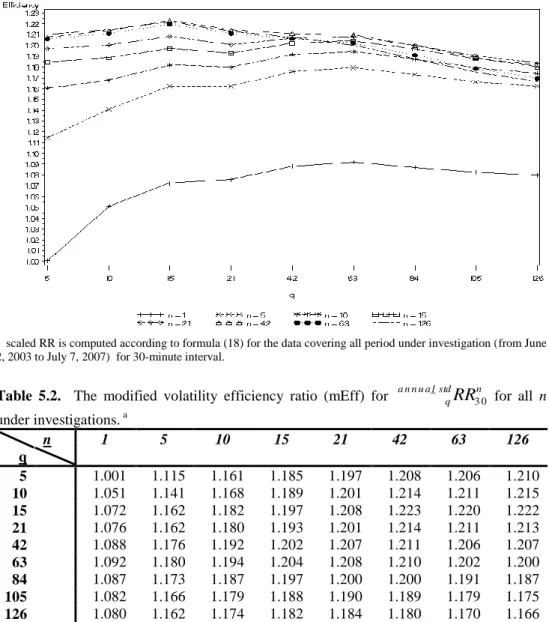
Figure 5.3. The modified volatility efficiency ratio (mEff) for a n n u a lstdq
RV
5n _for all n under investigations.a
a
scaled RV is computed according to formula (18) for the data covering all period under investigation (from June 2, 2003 to July 7, 2007) for delta = 5-minute interval.
Table 5.3. The modified volatility efficiency ratio (mEff) for a n n u a lstdq
RV
5n _for all n under investigations.a N 1 5 10 15 21 42 63 126 q 5 0.596 0.743 0.809 0.844 0.872 0.916 0.930 0.953 10 0.664 0.774 0.808 0.839 0.867 0.912 0.924 0.945 15 0.691 0.801 0.822 0.845 0.871 0.916 0.931 0.954 21 0.709 0.820 0.838 0.854 0.873 0.917 0.936 0.965 42 0.749 0.876 0.892 0.903 0.913 0.936 0.953 0.981 63 0.758 0.890 0.905 0.915 0.924 0.943 0.956 0.982 84 0.754 0.886 0.901 0.910 0.918 0.935 0.946 0.965 105 0.759 0.893 0.907 0.915 0.923 0.936 0.943 0.956 126 0.763 0.898 0.912 0.920 0.926 0.937 0.940 0.948 a scaled RV is computed according to formula (18) for the data covering all period under investigation (from June
2, 2003 to July 7, 2007) for delta = 5-minute interval.
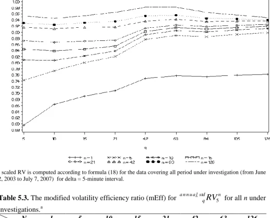
The figures 5.3-5.4 and tables 5.3-5.4 present the results for scaled RV with delta equals 5 and 30 minute for all n and all q. The selection of parameter q for scaled RV is the same as for scaled RR, i.e. q=63, what additionally confirms our previous selection.
Figure 5.4. The modified volatility efficiency ratio (mEff) for a n n u a lstdq
RV
3 0n _for all n under investigations.
a scaled RV is computed according to formula (18) for the data covering all period under investigation (from June
2, 2003 to July 7, 2007) for delta=30-minute interval.
Table 5.4. The modified volatility efficiency ratio (mEff) for a n n u a l_stdq
RV
3 0n for all n under investigations. n 1 5 10 15 21 42 63 126 q 5 0.648 0.790 0.857 0.891 0.917 0.958 0.971 0.997 10 0.701 0.823 0.861 0.892 0.919 0.963 0.974 0.998 15 0.723 0.848 0.873 0.896 0.922 0.969 0.984 1.012 21 0.737 0.865 0.889 0.907 0.926 0.972 0.992 1.027 42 0.768 0.918 0.940 0.952 0.963 0.992 1.016 1.053 63 0.771 0.925 0.947 0.958 0.968 0.995 1.016 1.053 84 0.769 0.924 0.947 0.958 0.966 0.988 1.006 1.036 105 0.772 0.929 0.951 0.961 0.969 0.989 1.002 1.027 126 0.774 0.935 0.956 0.966 0.972 0.988 0.998 1.017 a scaled RV is computed according to formula (18) for the data covering all period under investigation (from June2, 2003 to July 7, 2007) for delta = 30-minute interval.
After selecting q we focused on parameter n which was responsible for the length of the memory of the process. We had to solve some kind of the optimizing problem between long memory (high n) - smoothed volatility estimators with hardly any noise but low accuracy and short memory (low n) - volatile estimators which were highly infected by the noise factor but additionally characterized with high accuracy. We introduce the relative volatility efficiency ratio (rEff - formula (21)) in order to choose the best n maximizing the efficiency of the estimator regardless of delta parameter.
We base the process of selecting of parameter n on interval data equal 5- and 30-minute, which were found in the theoretical literature as the best compromise between:
1. maximizing the frequency of the data in order to get the best estimator of true volatility,
2. controlling the microstructure bias which increases significantly when we base our calculation on the interval sampled with the frequency which is too high.
We base the process of selection of n on the rEff instead of mEff because we want to make the comparison robust to the absolute values of standard deviation of our estimators.
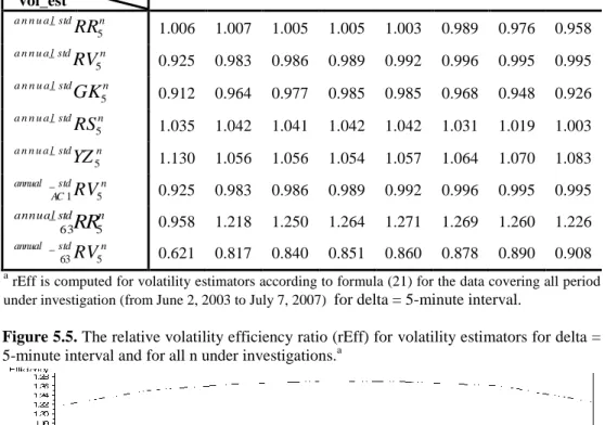
Table 5.5. The relative volatility efficiency ratio (rEff) for volatility estimators for delta = 5-minute interval and for all n under investigations.a
n 1 5 10 15 21 42 63 126 vol_est n std a n n u a l
RR
5 _ 1.006 1.007 1.005 1.005 1.003 0.989 0.976 0.958 n std a n n u a lRV
5 _ 0.925 0.983 0.986 0.989 0.992 0.996 0.995 0.995 n std a n n u a lGK
5 _ 0.912 0.964 0.977 0.985 0.985 0.968 0.948 0.926 n std a n n u a lRS
5 _ 1.035 1.042 1.041 1.042 1.042 1.031 1.019 1.003 n std a n n u a lYZ
5 _ 1.130 1.056 1.056 1.054 1.057 1.064 1.070 1.083 n std annual ACRV
5 _ 1 0.925 0.983 0.986 0.989 0.992 0.996 0.995 0.995 n std annualRR
5 _ 63 0.958 1.218 1.250 1.264 1.271 1.269 1.260 1.226 n std annualRV
5 _ 63 0.621 0.817 0.840 0.851 0.860 0.878 0.890 0.908 arEff is computed for volatility estimators according to formula (21) for the data covering all period under investigation (from June 2, 2003 to July 7, 2007) for delta = 5-minute interval.
Figure 5.5. The relative volatility efficiency ratio (rEff) for volatility estimators for delta = 5-minute interval and for all n under investigations.a
a rEff is computed from volatility estimators according to formula (21) for the data covering all period under
Tables 5.5-5.6 and figures 5.5-5.6 present the comparison criteria (rEff) necessary to select the most adequate n parameter. Basing on the same notion as before, for the consecutive comparisons, we chose n=42 and n=63 as the parameters maximizing the rEff and therefore minimizing standard deviation of our estimators.
Table 5.6. The relative volatility efficiency ratio (rEff) for volatility estimators for delta = 30-minute interval and for all n under investigations.a
n 1 5 10 15 21 42 63 126 vol_est n std a n n u a l
RR
3 0 _ 1.193 1.070 1.060 1.058 1.054 1.041 1.027 1.008 n std a n n u a lRV
3 0 _ 0.968 0.990 0.992 0.991 0.992 0.995 0.993 0.994 n std a n n u a lGK
3 0 _ 1.128 1.046 1.056 1.064 1.063 1.048 1.031 1.005 n std a n n u a lRS
3 0 _ 1.230 1.080 1.069 1.066 1.061 1.047 1.035 1.019 n std a n n u a lYZ
3 0 _ 1.260 1.063 1.047 1.041 1.040 1.042 1.042 1.046 n std annual ACRV
30 _ 1 0.968 0.990 0.991 0.991 0.992 0.995 0.993 0.994 n std annualRR
30 _ 63 1.005 1.291 1.329 1.347 1.355 1.357 1.346 1.295 n std annualRV
30 _ 63 0.602 0.840 0.872 0.887 0.898 0.922 0.940 0.961a rEff is computed for volatility estimators according to formula (21) for the data covering all period under
investigation (from June 2, 2003 to July 7, 2007) for delta = 5-minute interval.
Figure 5.6. The relative volatility efficiency ratio (rEff) for volatility estimators for delta=30-minute interval and for all n under investigations.a
a
rEff is computed for volatility estimators according to formula (21) for the data covering all period under investigation (from June 2, 2003 to July 7, 2007) for delta = 30-minute interval.
Having selected n and q parameters, finally, we came to the last step, i.e. the optimal sampling frequency selection (delta parameter). We based this step on the volatility estimators calculated for n=42 and n=63 (chosen in the last stage). The tables 5.8-5.9 and figures 5.8-5.9 present the relative volatility efficiency ratio (rEff) for n=42 and n=63 for all delta intervals under investigations.
Table 5.8. The relative volatility efficiency ratio (rEff) for volatility estimators for n=42 and for all delta interval under investigations.a
delta 5 10 15 30 60 105 210 420 vol_est 4 2 _
RR
std a n n u a l 0.989 0.998 1.018 1.041 0.979 1.024 1.020 1.049 4 2 _ RV
std a n n u a l 0.996 0.993 0.997 0.995 1.001 1.006 1.016 1.032 4 2 _ GK
std a n n u a l 0.968 0.984 1.019 1.048 0.948 1.008 1.001 1.027 4 2 _ RS
std a n n u a l 1.031 1.004 1.036 1.047 0.958 1.036 1.063 1.039 4 2 _ YZ
std a n n u a l 1.064 1.017 1.032 1.042 0.950 1.012 1.032 1.005 42 _ 1RV
std annual AC 0.996 0.993 0.997 0.995 1.001 1.006 1.015 1.032 42 _ 63RR
std annual 1.009 1.014 1.048 1.071 0.987 1.026 1.057 1.049 42 _ 63RV
std annual 1.002 1.007 1.045 1.053 0.986 1.041 1.062 1.032 a rEff is computed for volatility estimators according to formula (21) for the data covering all period underinvestigation (from June 2, 2003 to July 7, 2007) for n=42.
Figure 5.8. The relative volatility efficiency ratio (rEff) for volatility estimators for n=42 and for all delta interval under investigations.a
a rEff is computed for volatility estimators according to formula (21) for the data covering all period under
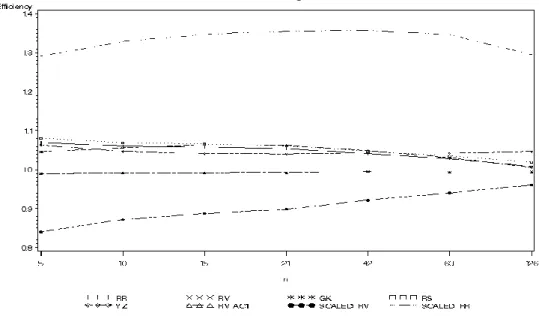
Table 5.9. The relative volatility efficiency ratio (rEff) for volatility estimators for n=63 and for all delta interval under investigations.a
delta 5 10 15 30 60 105 210 420 vol_est 6 3 _
RR
std a n n u a l 0.976 0.984 1.007 1.027 0.960 1.014 1.002 1.010 6 3 _ RV
std a n n u a l 0.995 0.994 0.996 0.993 0.997 1.000 1.004 1.013 6 3 _ GK
std a n n u a l 0.948 0.964 1.003 1.031 0.924 1.000 0.985 0.985 6 3 _ RS
std a n n u a l 1.019 0.990 1.026 1.035 0.936 1.030 1.050 0.997 6 3 _ YZ
std a n n u a l 1.070 1.017 1.037 1.042 0.941 1.016 1.030 0.976 63 _ 1RV
std annual AC 0.995 0.994 0.996 0.993 0.997 1.000 1.004 1.013 63 _ 63RR
std annual 1.002 1.005 1.042 1.062 0.971 1.017 1.041 1.010 63 _ 63RV
std annual 1.018 1.024 1.064 1.076 0.993 1.051 1.065 1.013 arEff is computed for volatility estimators according to formula (21) for the data covering all period under investigation (from June 2, 2003 to July 7, 2007) for n=63.
Figure 5.9. The relative volatility efficiency ratio (rEff) for volatility estimators for n=63 and for all delta interval under investigations.a
a rEff is computed for volatility estimators according to formula (21) for the data covering all period under
investigation (from June 2, 2003 to July 7, 2007) for n=63.
We chose delta = 30 (the parameter which maximizes rEff) as the best periodicity for the last stage of our research, i.e. the selection of the best estimator of true volatility. We noticed that the differences between efficiencies of consecutive estimators are not as
significant as it was presented in the previous papers (Martens and Dijk, 2007, Yang and Zhang, 2000, Garman-Klass, 1980, etc.) which introduced the new concepts of volatility estimators. The reason for this is that we compare the estimators with the same n, q and delta focusing only on their formulas.
We are also aware of the fact that the results show the relative efficiency in relation to standard deviation of annualized SD. Taking into account that we have the same benchmark (numerator in formula for mEff and rEff) while comparing our volatility estimators, such comparison should present stable results with respect only to the calculation formula employed.
After detailed process of selection we got nine estimators with two different values of n (42 and 63, which in practice does not influence significantly the properties of final estimator, see Tables 6.1-6.2 in the next section) and two different sampling frequencies (delta = 5, 30), which were let for consecutive comparison in order to accomplish our superior aim.
Before we come to the next section we have to stress a few interesting conclusions coming from the analysis presented above:
1. There is only a slight difference between the values of comparison criteria, which is in contrast to the results obtained in the process of previous researches indicating significant influence on efficiency of the estimator.
2. The amplitude of fluctuations of each comparison criterion differs significantly when we consider the selection of optimal n, q or delta, which additionally reveals the influence of each parameter on the final efficiency of the estimator.
3. We identified parameter n and delta as the most important for the final level of volatility.
Our results confirm the ones presented in financial literature where 5- to 30- minute intervals turn out to be the optimal sampling frequency. What is more important, the selection of parameter q (q=63) was similar to the presumptions of Martens and Dijk (2007). However, the most important value added of our research is the discussion of the optimal length of the memory of the process (parameter n), the issue which was not examined in the previous papers. This importance is even confirmed by the range of fluctuations of our comparison criteria when we try to choose the most appropriate n.
6. The distribution of different volatility measures
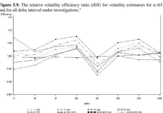
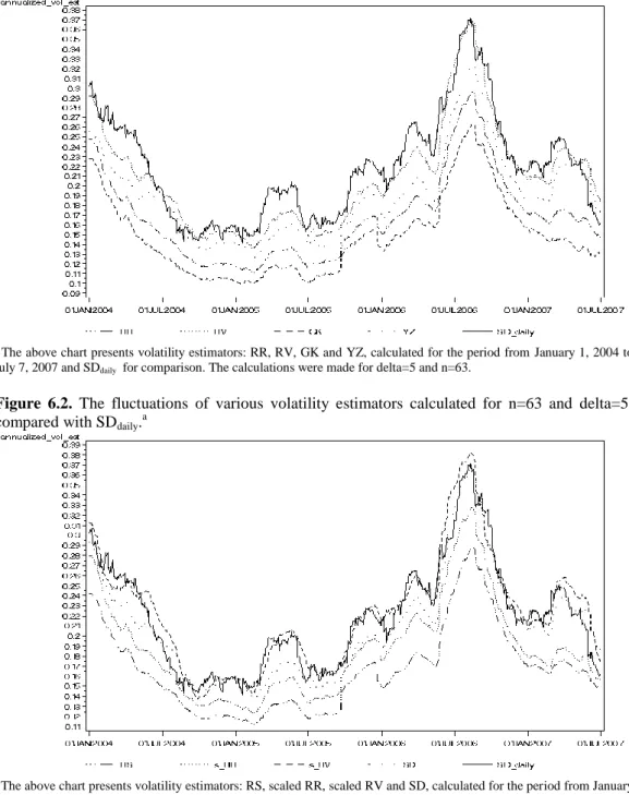
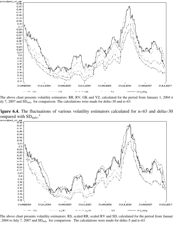
After the process of selection of essential parameter in the previous chapter we will carefully describe the properties of distribution of nine selected volatility measures, calculated on the ground of different theoretical notions, with respect to two different n and Δ. Moreover, we added the results for SD daily in order to reference our results to the benchmark widely used in volatility literature.
Tables 6.1-6.6 present the standard statistics of distributions, only for the parameters selected in the previous chapter. Additionally, we compare the results for delta=5, being the higher available frequency, which is the most connected to the true volatility which is instantaneous process.
The descriptive statistics for volatility estimators presented in this section were calculated for the period from November 28, 2003 to July 7, 2007. We have to leave 126 daily data (from June 3, 2003 to November 27, 2003) because such amount is required to calculate the first value of annualstd n
RR
_ 63 and n std annual RV _63 (63 daily data for scaled parameter and 63 in