Accounting for Consumption and Saving in the United
States: 1960-2004
Kaiji Chen
†Ay¸se
˙
Imrohoro
˘
glu
‡Selahattin
Imrohoro
˙
˘
glu
‡First Version October 2005; This Version October 2006
Abstract
The saving rate in the U.S. has been declining since the 1960s while the share of consumption in output has been increasing. We examine whether standard growth the-ory can explain the behavior observed between 1960-2004. We use an infinite horizon, complete-markets growth model calibrated to U.S. data and show that the model gener-ates saving rgener-ates and consumption-to-output ratios that are resonably similar to the data during 1960-2004. The secular decrease in the population growth rate and the increase in the depreciation rate are significant in explaining the trends, where as the medium term fluctuations in the total factor productivity seem important in driving the year-to-year movements in macroeconomic aggregates.
∗Department of Economics, University of Oslo
‡Department of Finance and Business Economics, Marshall School of Business,
1
Introduction
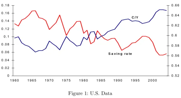
Understanding the secular trends in consumption and saving in the U.S. has been an im-portant part of academic research. It has also occupied center stage in policy discussions and media coverage. Figure 1 displays the changes in consumption to output ratio and the saving rate in the U.S. between 1960-2004.1
C o n s u m p tio n a n d S a v in g in th e U .S . 0 0 . 0 2 0 . 0 4 0 . 0 6 0 . 0 8 0 . 1 0 . 1 2 0 . 1 4 0 . 1 6 0 . 1 8 1 9 6 0 1 9 6 5 1 9 7 0 1 9 7 5 1 9 8 0 1 9 8 5 1 9 9 0 1 9 9 5 2 0 0 0 Sa v in g R a te 0 . 5 2 0 . 5 4 0 . 5 6 0 . 5 8 0 . 6 0 . 6 2 0 . 6 4 0 . 6 6 C/ Y C / Y S a v i n g r a te
Figure 1: U.S. Data
Why has the national saving rate declined between 1960-2004, and why does the U.S. save less than other developed economies? Gokhale, Kotlikoff, and Sabelhaus (1996) attribute the decline in the net national saving rate to the redistribution of resources, though social security and medicare, from young consumers with low marginal propensities to consume to older generations with high marginal propensities to consume. Several papers explore whether particular cohorts are responsible for the low saving rate by examining personal saving rates in the U.S.2 Attanasio (1998) argues that cohorts born between 1925 and 1939 may be to blame for the low personal saving rate. Summers and Carroll (1987) suggest that it is the reliance of the younger generations on social security that depresses saving in the U.S. Boskin and Lau (1988a,b) formulate a model based on longitudinal and cross-sectional microeconomic data together with aggregate time series and examine the importance of
1C/Y is the fraction of consumption in GNP, and the saving rate is net national saving as a percent of
net national income. In the appendix we explain the adjustments that were made to the data to ensure consistency between the data and the model.
2
various factors affecting aggregate consumption and saving in the U.S. Their results suggest that it is the decline in the saving of generations born after the great depression that may be responsible for the decline in the national saving rate.3
In this paper we explore the quantitative implications of growth theory on the secular trends in the net national saving rate and the consumption output ratio in the U.S. between 1960 and 2004. Our approach is in line with the recent use of the one-sector growth model to explain ‘Great Depressions’. In particular, we follow the methodology of Cole and Ohanian (1999) and Kehoe and Prescott (2002) in using an applied general equilibrium setup to account for the observed time path of the U.S. saving and consumption behavior.4 We use a standard one-sector, neoclassical growth model with an infinitely-lived representative agent facing complete markets and calibrate the economy to the U.S. data for the 1960-2004 period. Our exogenous driving forces are the population growth rate, the tax rates on capital and labor income, the share of government expenditures in output, the depreciation rate, and the actual time series data for the TFP growth rate. We conduct deterministic simulations, as in Hayashi and Prescott (2002), and perform an ‘accounting exercise’ to evaluate the impact of several factors that may explain the secular trends in the saving and consumption behavior the U.S. Our results suggest that the one sector growth model can generate the secular trends in the consumption and the saving behavior reasonably well once the actual time paths of TFP growth rate, population growth rate, and the depreciation rate are taken into account.
The paper is organized as follows. Section 2 presents the growth model we use to evaluate U.S. consumption and saving behavior. Data and calibration issues are discussed in Section 3, and the quantitative findings are presented in Section 4. Concluding remarks are given in Section 5. Appendix A contains calibration details and data sources.
1.1
The Growth Model
There is a stand-in household with Nt working-age members at date t. The size of the
household evolves over time exogenously at the rate nt = Nt/Nt−1. In this framework a
3Another set of papers have focused on the possible relationship between the increase in stock prices and
the boom in consumer spending. For example, see Parker (1999), Juster, Lupton, Smith, and Stafford (2000)
who suggest that the significant capital gains in corporate equities experienced since 1984 is responsible for
representative household solves max ∞ X t=0 βtNt(logct+αlog(1−ht)) subject to Ct+Xt≤(1−τh,t)wtHt+rtKt−τk,t(rt−δt)Kt+T Rt−πt,
where ct =Ct/Nt is per member consumption, ht= Ht/Nt is the fraction of hours worked
per member of the household,β is the subjective discount factor, αis the share of leisure in the utility function, Htis total hours worked by all working-age members of the household,
τh,t andτk,t are tax rates on labor and capital income, respectively, at timet, wtis the real
wage, T Rt is a government transfer, πt is a lump sum tax, rt is the rental rate of capital,
and δt is the time-t depreciation rate. Households are assumed to own the capital,Kt, and
rent it to businesses. The economy-wide resource constraint is given by
Ct+Xt+Gt=Yt,
where aggregate consumption, investment and government purchases add up to aggregate output. The law of motion for the capital stock is given by Kt+1 = (1−δt)Kt+Xt.
The aggregate production function is given by
Yt=AtKtθ(Ht)1−θ,
where θ is the income share of capital and At is total factor productivity, which grows
exogenously at the rate gt=At/At−1.
1.2
Government
There is a government that taxes income from labor and capital (net of depreciation) and uses the proceeds tofinance exogenous streams of government purchasesGtand government
transfers T Rt.A lump sum tax πt is used to ensure that the government budget constraint
is satisfied each period:
Gt+T Rt=τh,twHt+τk,t(rt−δt)Kt+πt.
In other words, πt is the primary government deficit in the model.
1.3
Competitive Equilibrium
Given a government policy {Gt, T Rt, τh,t, τk,t, πt}∞t=0, a competitive equilibrium consists of
• given policy and prices, the allocation solves the household’s problem,
• given policy and prices, the allocation solves the firm’s profit maximization problem with factor prices given by: wt= (1−θ)AtKtθ(Ht)−θ,and rt=θAtKtθ−1(Ht)1−θ, • the government budget is satisfied,
• and the goods market clears: Ct+Xt+Gt=Yt.
1.4
Numerical Solution
Our numerical solution procedure follows Hayashi and Prescott (2002). After calibrating the model parameters and exogenous variables, wefirst compute a steady-state assumed for the U.S. economy in the sufficiently distant future. To obtain this steady-state, we write down the equilibrium conditions of the model, detrend variables to induce stationarity, and then impose these steady-state conditions. Once the steady-state is obtained, we use a shooting algorithm toward this final steady state from given initial conditions in 1960. This solution method yields an equilibrium transition path from initial conditions toward a steady-state.
Equilibrium Conditions: The equilibrium conditions of this model can be described in two equations below:
Ct+1 Nt+1 = Ct Nt β n 1 + (1−τk,t+1) h θAt+1Ktθ+1−1(Ht+1)1−θ−δt+1 io , (1) Kt+1 = (1−δt)Kt+AtKtθ(Ht)1−θ−Ct−Gt. (2) Detrending: For an aggregate variable zt, its detrended version is given by: ezt =
zt/ ∙ A 1 1−θ t Nt ¸
.Applying this change of variables, we obtain equations
e ct+1 = e ct gt βn1 + (1−τk,t+1) h θxθt+1−1−δt+1 io , e kt+1 = 1 gtnt [(1−δt) + (1−ψt)xtθ−1]ekt−ect,
whereψt is the ratio of government purchases to output,Gt/Yt,andxt is detrended
capital-labor ratio,(Kt/Ht)/A 1 1−θ t .
respectively. The steady-state saving rate is given by
e
s= (gn−1)ek
e
y−eδek . (3)
Transition to the steady-state: Starting from a given value of the initial capital stock K0,we guess a value for the endogenous variableC0 and use equations (1)and(2)to obtain
a path for the endogenous variables Ct and Kt+1 towards the steady-state. If this path
is not achieved, we iterate on the initial guess for C0 using this ‘shooting’ algorithm until
convergence to the steady-state is obtained. Equipped with the equilibrium path of Ct and
Kt+1,we can then use other equilibrium conditions to construct time paths of all aggregate
quantities and prices. In particular, we compute the saving rate using5
st=
Yt−Gt−Ct−δtKt
Yt−δtKt
.
2
Calibration
We calibrate the model economy using data from the 2005 revision of National Income and Product Accounts (NIPA), Fixed Asset Tables (FAT) of Bureau of Economic Analysis (BEA), Statistics of Income (SOI), Individual Income Tax Returns (1960-2003), and the Social Security Bulletin.
Constant Parameters: There are 3 parameters that are time invariant throughout our analysis. The capital share parameter, θ, is set to its average value of0.4 over our sample period 1960-2004. The subjective discount factor, β, is set to 0.9702 so that the capital output ratio is 3.2 at the final steady state. The share of leisure in the utility function, α, is set to 1.45 to match an average workweek of 35 hours. These choices are summarized below.
Time-Invariant Parameters θ 0.4 1960-2004 average
β 0.9702 Target: K/Y = 3.2in steady state α 1.45 Target: Average workweek = 35hours
Calibration of the Steady-State (2070 and Beyond) and 2005-2070: We assume that the U.S. economy starts from given conditions in 1960 and eventually converges to a
5We treat the model as a closed economy where net national saving and invsetment are identical. Figure
?? in the Appendix displays the net national saving and investment rates for the U.S. economy in this time period. As expected, after the 1980s there is a divergence between the two series indicating the current
accounts deficits in the U.S. Perhaps a two country model for that time period would be useful especially
if the aim is to understand the current account deficits of that period. For the purposes of this model, the
steady-state in 2070.6 In order to characterize this steady-state equilibrium, we use the following values for model variables, starting from year 2005:
Steady-State Values: 2005 and Beyond
gt−1 TFP Growth Rate 0.0142
nt−1 Population Growth Rate 0.01
ψt Government Purchases to GNP Ratio 0.14
δt Depreciation Rate 0.05
T Rt/GN P Transfers to GNP Ratio 0.10
τk,t Capital Income Tax Rate 0.40
τh,t Labor Income Tax Rate 0.276
In our benchmark model, we set the seven exogenous variables in the above list equal to their long-run averages.7 Note that the population growth rate in the U.S. has been declining since the 1960s and according to the Census Bureau projections it will continue at very low rates in the future. Thus, we set the population growth rate after 2004 and at the steady state equal to 1% which is smaller than the average population growth rate of1.5%
between 1960-2004.8 Similarly, the depreciation rate has been increasing in the U.S. For the periods after 2004 and at the steady state, we set the depreciation rate equal to5%which is the average depreciation rate between 1990-2004.9 We discuss the sensitivity of our results
to the assumptions made for the periods beyond 2004 in the section on sensitivity analysis.
Calibration of the 1960-2004 period: In our benchmark simulation, we use the actual time series data between 1960-2004 for the following exogenous variables: TFP growth rate, population growth rate, depreciation rate, share of government purchases in GNP, share of government transfers in GNP, and capital and labor income tax rates. 10 Empirical tax
rates are constructed using the methods of Joines (1981) and McGrattan (1994). The data
6This is an approximation. Allowing for a longer transition period from 1960 for convergence to a
steady-state has no quantitative impact on the 1960-2004 period we are investigating.
7With our assumed tax rates, the government budget will be in a surplus at the steady state.
8Population growth rates are obtained from the BLS and are the growth rates of civilian non-institutional
used in the calibration are provided in the Appendix. We compute the initial capital-output ratio in 1960 as 3.5and take it as a given initial condition.
1960-2004 Values: Benchmark Model with Time-Varying Exogenous Variables
gt−1 TFP Growth Rate Authors’ Calculations
nt−1 Population Growth Rate Authors’ Calculations
ψt Government Purchases to GNP Ratio Authors’ Calculations
δt Depreciation Rate Authors’ Calculations
T Rt/GN P Transfers to GNP Ratio Authors’ Calculations
τk,t Capital Income Tax Rate Authors’ Calculations
τh,t Labor Income Tax Rate Authors’ Calculations
3
Results
3.1
Main Findings
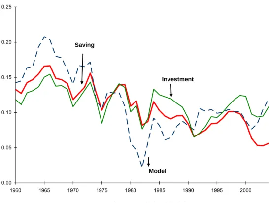
We start this section by a comparison of the key macroeconomic aggregates that are gen-erated by the model against their empirical counterparts. Since we assume closed economy, there is no distinction between saving and investment in our model. In Figure 2 we display the data for net national saving rates and the ratio of net domestic investment to NNP, as well as the model generated saving rate. First, the observed saving and investment rates seem to display similar fluctuations in this time period. In two subperiods, late 1980s and late 1990s, the rate of investment is larger than the saving rate, highlighting the current account deficits in the U.S. for these periods. Since the focus of our paper is the saving rate, we will compare our model’s simulated saving rate with the empricially calculated saving rate.
ment and the current account surplus. Even though, we treat the model as a closed economy, we include
the foreign capital in the definition of the capital stock to make sure that the TFP growth rates faced by
the U.S. individuals can be accurately measured. However, it is important to note that this adjustment is
quantitatively very small. None of the results are significantly altered by different measurements of TFP such
as inclusion of government capital or the exclusion of foreign capital. Gomme and Rupert (2005) provide
three different measures on the U.S. TFP growth rate based on very different assumptions on the capital
stock. The TFP growth rates implied by their results as well as ours display very similar properties over this time period.
0.00 0.05 0.10 0.15 0.20 0.25 1960 1965 1970 1975 1980 1985 1990 1995 2000 Sa ving an d I n ves tmen t Saving Model Investment
Figure 2: Data and the Model
The simulated saving rate is given in Figure 2 with the series labeled ‘model’. The model does reasonably well in terms of capturing some of the movements in the actual U.S. data. However, the model generated saving rate is considerably larger than the data in the mid 1960s and smaller than the data between 1975 and 1990.
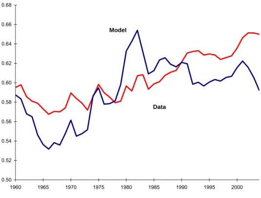
Figure 3 displays the actual and simulated consumption-output ratios which exhibit a similar fit. Although the secular movements seem to be reasonably characterized, the model has difficulty mimicking the observed behavior in certain subperiods.
0.50 0.52 0.54 0.56 0.58 0.60 0.62 0.64 0.66 0.68 1960 1965 1970 1975 1980 1985 1990 1995 2000 C/Y Data Model
Figure 3: Consumption-Output Ratio
In order to understand the main factors behind the behavior of consumption and saving over this time period, we conduct several counterfactual experiments. In our benchmark economy, we have used time series data for the TFP growth rate, population growth rate, depreciation rate, capital and labor income tax rates, and fraction of government expendi-tures in GNP. There are particularly significant changes in the population growth rate which declines from 1.6% to 1.0%, and the depreciation rate which increases from 4.3% to 5.2% between 1960 and 200411. In addition, capital income tax declines from 44% to 33% and the labor income tax increases from 23% to 27%. To isolate the impact of these changes one at a time we start with setting all the exogenous variables equal to their sample averages. Later we add the time series data for each exogenous variable one at a time.
Population Time Series Only: In ourfirst counterfactual experiment we try to isolate the role of the declining population growth rate by simulating the saving rate in an economy where all the exogenous variables (TFP growth, G/Y, depreciation, tax rates, transfers) are set to their long-run averages except for the population growth rate. In Figure 4, we display the saving rate from the data labeled ‘data’. The series labeled ‘Population Time Series Only’ displays the saving rate that is generated by the model economy where the only time series data that is used in the simulations is the population growth rate. The quantitative
1 1Figures A2 and A3 in the appendix display the changes that took place in some of the exogenous variables
impact of the population growth rate in this time period seems fairly small, resulting in a 1% decline (from 12% in 1960 to 11% in 2004). The largest decline is from 14.3% in 1970 to 11.6% in 2004. 0.04 0.06 0.08 0.10 0.12 0.14 0.16 0.18 1960 1965 1970 1975 1980 1985 1990 1995 2000 Savi ng R a te Data
Population Time Series Only
Figure 4: Role of Population Growth
Declining Population Growth Rate and Increasing Depreciation Rate: In Fig-ure 5 we conduct an experiment that quantifies the role of the population growth rate together with the depreciation rate. Our calibration has indicated a slight increase in the depreciation rate which alone would result in a decrease in the saving rate. The series labeled ‘Time Series for population and depreciation’ display the results of this experiment. The increase in the depreciation rate and the decrease in the population growth rate together result in a quantitatively significant decline in the saving rate between 1960 and 2004, about 3 percentage points.
0.04 0.06 0.08 0.10 0.12 0.14 0.16 0.18 1960 1965 1970 1975 1980 1985 1990 1995 2000 Savi ng R a te
Time Series for population and depreciation
Data
Figure 5: Role of the Population Growth and Depreciation
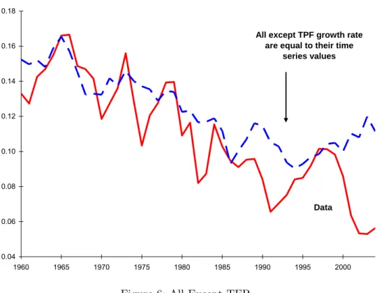
All Time-Varying Except TFP Growth Rate: In Figure 6 we generate the saving rate in an economy where time series values of all the exogenous variable except the TFP growth rate are used in the simulations. Thus in this environment, tax rates, transfers, population growth rate and the depreciation rate all take their time series values whereas the TFP growth rate is set to its long-run average. Notice that the resulting saving rate is able to capture some of the secular decline in the saving rate. However, the simulated saving rate does generate the decline observed in the data in late 1980s and late 1990s.
0.04 0.06 0.08 0.10 0.12 0.14 0.16 0.18 1960 1965 1970 1975 1980 1985 1990 1995 2000 Sa vi ng R a te Data All except TPF growth rate
are equal to their time series values
Figure 6: All Except TFP
TFP Growth Rate Only: Next, we examine the model generated saving rate when the only time series data that is included in the simulations is the TFP growth rate. We set all the other exogenous variables equal to their long-run averages. There are several interesting features of the model generated saving rate that is displayed in Figure 7. First, it displays significantfluctuations that mimic the data rather well until 1975. There is a sharp decline in the model generated saving rate in the early 1980s and late 1990s, and a sharp increase in the early 1990s.
0.00 0.02 0.04 0.06 0.08 0.10 0.12 0.14 0.16 0.18 0.20 1960 1965 1970 1975 1980 1985 1990 1995 2000 Sav ing R a te Data
TFP Time Series Only
Figure 7: Role of TFP
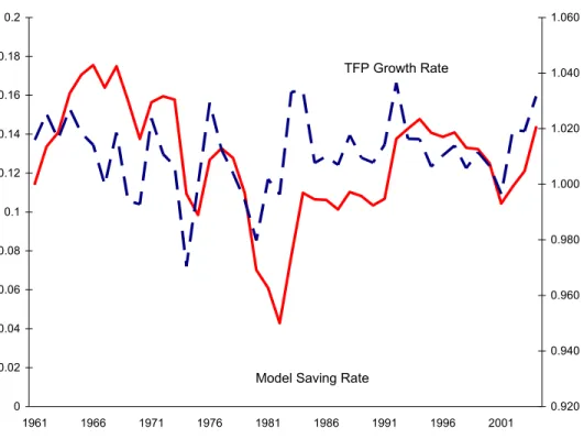
To understand the relationship between TFP growth and the saving behavior better, we display these two series in Figure 8. Since we are conducting deterministic simulations, households know the entire path of the TFP growth rate and make decisions on how much to save based on this information. In general, periods with high TFP growth are associated with high return to capital and high saving rates. For example, the model generates a relatively high saving rate between 1990-1995 which is a period of relatively high TFP growth. The decline in the TFP growth rate in 2001 results in a sharp decline in the saving rate.
0 0.02 0.04 0.06 0.08 0.1 0.12 0.14 0.16 0.18 0.2 1961 1966 1971 1976 1981 1986 1991 1996 2001 Sav ing Rate 0.920 0.940 0.960 0.980 1.000 1.020 1.040 1.060 T F P gr ow th r a te
Model Saving Rate
TFP Growth Rate
Figure 8: TFP Growth and the Saving Rate
Overall, our results suggest thati) the secular decline observed in the U.S. since 1960s is mostly due to the decline in the population growth rate and the increase in the depreciation rate, ii) observed TFP growth rates alone would have caused the saving rate to be much higher in the 1990-1995 period, and, iii) the decline in the TFP growth rate in 2001 had a significant negative impact on the saving rate.
3.2
Additional Properties and Sensitivity Analysis
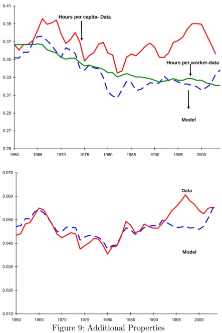
Labor Input and Return to Capital: In this section we examine additional properties of the benchmark economy by comparing the simulated series for labor, capital and the interest rate with their counterparts in the data. Our results indicate that the model economy works reasonably well in mimicking some aspects of the data but not all. In Figure 9 we display the observed time series path of the labor input and the after-tax return to capital (calculated
the reason why observed total hours did not decline. In our simple model, the decrease in simulated hours is mainly driven by the fact that tax rates on labor increase steadily over the past forty years. Therefore, with perfect anticipation of this trend, the stand-in household tends to substitute hours in the early periods for hours in the late periods.
In the second panel, we display the after-tax rate of return to capital in the data and the model economy. Although the fit from 1960 to 1990 appears tight, there is a major discrep-ancy between the two series in the 1990s. One potential reason for such a big discrepdiscrep-ancy is that in the 1990s capital’s share in total income increases a lot, while in our model it is constant due to the Cobb-Douglas production specification. Notice that the after-tax rate of return for capital in the data is positively correlated with capital share in total income and negatively correlated with the capital-output ratio, while in our model it is driven by capital-output ratio alone. Therefore, given that capital’s share in total income increases during the 1990s, our model tends to underestimate the increase in the after-tax return to capital.
0.25 0.27 0.29 0.31 0.33 0.35 0.37 0.39 0.41 1960 1965 1970 1975 1980 1985 1990 1995 2000 Labo r Model Hours per capita- Data
Hours per worker-data
0.010 0.020 0.030 0.040 0.050 0.060 0.070 1960 1965 1970 1975 1980 1985 1990 1995 2000 After T a x Net Retu rn to C a pital Model Data
Figure 9: Additional Properties
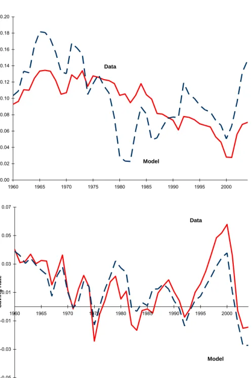
Private and Public Saving Rates: It is also possible to separate the net national saving rate in this economy into its two components and examine the private and the gov-ernment saving rates separately. In Figure 10 we display the simulated series against their counterparts in the data. Notice that while the simulations take the tax rates and the
high in 2004. 0.00 0.02 0.04 0.06 0.08 0.10 0.12 0.14 0.16 0.18 0.20 1960 1965 1970 1975 1980 1985 1990 1995 2000 Pri vate Savi n g R a te Data Model -0.05 -0.03 -0.01 0.01 0.03 0.05 0.07 1960 1965 1970 1975 1980 1985 1990 1995 2000 Go ve rnm e n t Sa vi n g Ra te Data Model
Figure 10: Private and Government Saving
Alternative Assumption on Values for 2005 and Beyond: Our procedure for assigning values to TFP growth rates between 2005 and thefinal steady-state is arbitrary. In our benchmark calculations we set the TFP growth rate equal to its 1960-2004 average right after 2004. To check the sensitivity of our results to this assumption, we report simulations from a case where we assume the TFP growth rate to continue at its 2004 level which is higher than its steady state value. In Figure 11, the vertical line represents the year 2004
beyond which the two simulated saving rates differ only because of the assumed values for the TFP growth rate for 2005 and beyond. The two series are virtually identical until 1990s. There are noticeable difference in the 1990-2004 period between the two series, however, both capture the increase in the saving rate and the decline in C/Y that takes place in this period. As Figure 11 shows, the implications of the TFP growth rate beyond 2004 significantly differ between the two simulations.
0.00 0.05 0.10 0.15 0.20 0.25 1960 1970 1980 1990 2000 2010 Sa v ing R a te High future TFP Low future TFP Data 0.56 0.58 0.60 0.62 0.64 0.66 0.68 C/ Y High future TFP
3.3
No Perfect Foresight
So far we assume perfect foresight. Households know the entire time path of all exogenous variables. Hayashi and Prescott (2002) and Chen, ˙Imrohoroglu, and˘ Imrohoro˙ ˘glu (2006) argue that this assumption plays a quantitatively minor role in the model’s ability to generate empirically plausible aggregates. In this section, we will summarize the our findings from two alternative assumptions on expectations for the TFP growth rate.
Adaptive Expectations: Ourfirst alternative expectations scheme is a simple adaptive framework where expectations of future TFP growth rates are formed according to
get+1 =gte+λ(gt−gte).
Here, the parameter λ∈ [0,1]< reflects the extent to which expectations will change as a result of past errors. Aλnear zero indicates near-static expectations whereas aλnear unity suggests setting expectations equal to the most recently observed actual growth rate. In the latter case, the model’s saving rate would essentially shift one period hence relative to our perfect foresight case.
0 0.02 0.04 0.06 0.08 0.1 0.12 0.14 0.16 0.18 0.2 1960 1965 1970 1975 1980 1985 1990 1995 2000 2005 Saving R a te λ=0.2 λ=0.4 Data
Figure 12 displays observed saving rates and a collection of simulated saving rates indexed by a few values of λ. Even the near-static expectations cases with low values of λgenerate saving rates with similar features compared to the deterministic case. The secular movements are reasonably well-represented, but the model does a poor job in the 1980s and early 2000s.
Stochastic TFP Growth Rate: Another alternative formulation is to assume that TFP growth rate follows an AR(1) process. Estimating this simple process yields a per-sistence coefficient of 0.33 (with an intercept term 0.69 and a standard error of regression 0.0224). 0 0.02 0.04 0.06 0.08 0.1 0.12 0.14 0.16 0.18 1960 1965 1970 1975 1980 1985 1990 1995 2000 2005 Savi ng R a te Data AR(1) TFP growth
Figure 13: Saving Rate with AR(1)
Figure 13 depicts the actual saving rate and the model generated saving rate when households forecast future TFP growth rates using the estimatedAR(1)process given above.
4
Concluding Remarks
Why has the U.S. net national saving rate fallen from about 14 percent in 1960s to about 6 percent in early 2000s? A popular answer has been the decline in the private saving of the baby boom generation in response to an increase in the generosity of the social security program. In this paper, we abstract from life cycle features and social security, and employ a standard growth model calibrated to the U.S. economy. Our infinite horizon, complete markets setup captures the decline in the U.S. saving rate reasonably well. The important factors responsible for the secular decline between 1960 and 2004 are i) the decrease in the population growth rate, ii) the increase in the depreciation rate, and, iii) the increase in the labor income tax rate. The time path of observed TFP growth rates does not exhibit a trend but help explain the year-to-yearfluctuations in the saving rate over this time period. Although the standard model performs well overall, the results for the periods after 1990 are sensitive to the assumptions made about the future. The model also abstracts from several features on the U.S. economy that seem to be important especially since the 1990s. For example, McGrattan and Prescott (2006) document the importance of intangible capital since 1990s that is absent in our calculations. In addition, the model we have used can not account for the large increase in household wealth and its possible impact on the saving consumption decision. These issues, and a more detailed study of the 1990s is left for future research.
5
Appendix
5.1
Calibration of the Benchmark Economy
In this section, we provide the details of our calibration for the benchmark economy. We use data from the 2005 revision of National Income and Product Accounts (NIPA) and Fixed Asset Tables (FAT) of Bureau of Economic Analysis (BEA) for the years 1960-2004. Our adjustments to measured macroeconomic aggregates follow Cooley and Prescott (1995).
Denote measured GNP as follows
(cs+cnd+icd) +g+i+nx+nf p=GN P =dep+N N P (A-1)
wherecs, cnd, icddenote serviceflow of consumer durables, consumption of nondurable and expenditure on consumer durable. g denotes the sum of government consumption, denoted as gc, and gross government investment, denoted asgi. i denotes gross private investment. nx denotes net export and nf pdenotes net factor payments on foreign assets. dep denotes consumption offixed capital.
include the serviceflow from government capital,sg, A-1 becomes
(cs+cnd+icd+sg) +gc+ (i+gi) +nx+nf p=GN P +sg=dep+ (N N P +sg) (A-2)
where dgi denotes depreciation of government fixed assets and dep−dgiis depreciation of privatefixed asset.
Second, we treat the stock of consumer durable as part of capital stock. Then A-2 becomes
(cs+cnd+csd+sg) +gc+ (i+nicd+dcd+gi) (A-3)
+nx+nf p = GN P +sg+csd
= (dep+dcd) + (N N P +sg+csd−dcd)
where csd is service flow from consumer durable anddcd denote depreciation of consumer durable. Therefore, total private consumption becomes (cs+cnd+csd+sg) and total investment investment becomes(i+icd+gi)or(i+nicd+dcd+gi), wherenicdis referred to as net investment in consumer durable anddcddenotes depreciation of consumer durable. Total depreciation becomes(dep+dcd).
Third, we treat net foreign asset as part of capital stock. A-3 then becomes
(cs+cnd+csd+sg) +gc (4)
+(i+nicd+dcd+gi+nx+nf p) = GN P +sg+csd (5)
= (dep+dcd) + (N N P +csd+sg−dcd)
Now total investment becomes (i+nicd+dcd+gi+nx+nf p).
In summary, we define capital K as the sum of the fixed assets, stock of consumer durables, inventory stock land, and net foreign assets. Output Y corresponds to GN P +
sg+csd and total depreciation corresponds to dep+dcd.
Following McGrattan and Prescott (2000), we assume that the rate of returns for con-sumer durable and government fixed assets are equal to the rate of return for non-corporate capital stock. Specifically, we have
i = (Accounting Returns + Imputed Returns)
(Non-corporate capital +land+inventory+Capital of Foreign Subsidiary) (0.0603 + 1.6803i)
Ysd and Ysg denote the service flows from consumer durables and government capital,
respectively, which are computed following Cooley and Prescott (1995).
Ysd = csd= (i+δd)KD
Ysg = (i+δg)KG
Then the capital share in the output function αis computed as
α= Ykp+Ysd+Ysg
GN P +Ysd+Ysg
, where Ykp is the income from private fixed assets
Ykp = Unambiguous capital income+θp×(proprietors’ income (A-5)
+indirect business tax)+depreciation (6)
= θp×GN P
This gives a value 0.32 forθp and a value of0.41 forα.
Define the net national saving rate as
s = Y −CON −GOV −DEP R
Y −DEP R
= (GN P +sg+csd)−(cs+cnd+csd+sg)−gc−(dep+dcd) (GN P +sg+csd)−(dep+dcd)
= GN P −cs−cnd−gc−(dep+dcd)
N N P +csd+sg−dcd
Since in our model government does not issue debt or lend to households, we define the primary government saving rate as
sgov= Tax revenue−(gc+tr)−net interest payment on government liability
Y −DEP R
where tr is the net government transfer, computed as current transfer payment minus current transfer receipts. Accordingly, the private saving rate is computed as
psav =s−sgov TFP level is computed as
A= Y
Table A1. Model Economy Account Model Expression 1 Depreciation δK 2 Labor income wH 3 Capital income rK 4 Total Income Y 5 Private Consumption C 6 Government Consumption G 7 Investment I 8 Total Product Y
Table A2. National Accounts, Average 1960-2003 Relative to GNP
Consumption offixed capital 0.115
Compensation of employees 0.571
Unambiguous capital income13 0.154
Proprietors’ Income with IVA and CCadj 0.074
Indirect Business Taxes14 0.086
Gross national income 1.000
Personal consumption expenditures 0.635
Durable goods 0.082
Nondurable goods and services 0.553
Gross private domestic investment 0.161
Government consumption expenditures and gross investment 0.206
Consumption expenditures 0.167
Gross investment 0.039
Net foreign investment15 -0.002
Gross national product 1.000
Addendum
Consumption offixed capital, durable goods 0.062 Consumption of governmentfixed assets 0.024 Net stock of governmentfixed assets 0.671 Net stock of consumer durable goods 0.301
1 3Unambiguous capital income=Rental Income of persons with CCAdj+Corporate Profits with IVA and
CCadj+Net Interest and miscellaneous payments.
1 4
Indirect business taxes are equal to the sum of tax on production and imports less subsidies, business transfer, current surplus of government enterprises and statistical discrepancy.
1 5
Table A3. Mapping From National Accounts to Model Accounts (Excluding Gov’t Capital)
Model NIPA
1 Depreciation (δK) 0.153
Consumption offixed capital 0.115
Consumption offixed capital, durable goods 0.062 Less: Consumption of governmentfixed assets -0.024
0.153
2 Labor income (wE) 0.683
Compensation of employees 0.571
0.7×(Proprietors’ income +Indirect business taxes) 0.112 0.683
3 Capital income (rK) 0.228
Unambiguous capital income 0.154
0.3×(Proprietors’ income +Indirect business taxes) 0.048 Imputed capital services from durable goods 0.026 0.228
4 Total income (Y) 1.064 1.064
Table A3. Mapping From National Accounts to Model Accounts (Excluding Gov’t Capital)
5 Private consumption(C) 0.641
Personal consumption expenditure 0.635
Less: Consumption expenditure, durable goods -0.082
Imputed capital ser. from durable goods16 0.026
Consumption offixed capital, durable goods 0.062 0.641
6 Public consumption (G) 0.182
Government consumption exp. and gross investment 0.206 Less: Consumption of fixed capital, gov. capital -0.024
0.182
7 Investment (I) 0.241
Gross domestic private investment 0.161
Personal consumption expenditure, durable goods 0.082
Table A4. Mapping From National Accounts to Model Accounts (Including gov’t capital)
Model NIPA
1 Depreciation (δK) 0.177
Consumption offixed capital 0.115
Consumption offixed capital, durable goods 0.062 0.177
2 Labor income (wH) 0.683
Compensation of employees 0.571
0.7×(Proprietors’ income+Indirect business taxes) 0.112 0.683
3 Capital income (rK) 0.286
Unambiguous capital income 0.154
0.3×(Proprietors’ income+Indirect business taxes) 0.048 Imputed capital services from durable goods 0.026 Imputed services from government fixed assets 0.058 0.286
4 Total income (Y) 1.146 1.146
Table A4 Mapping From National Accounts to Model Accounts (Including gov’t capital)
5 Private consumption (C) 0.699
Personal consumption expenditure 0.635
Less: Consumption expenditure, durable goods -0.082 Imputed capital services from durable goods 0.026 Imputed services from government capital17 0.058 Consumption offixed capital, durable goods 0.062 0.699
6 Public consumption (G) 0.167
Government consumption expenditure 0.167
7 Investment (I) 0.280
Gross domestic private investment 0.161
Personal consumption expenditure, durable goods 0.082
Net foreign investment -0.002
Gross government investment 0.039
0.280
8 Total Product (Y) 1.146 1.146
1 7
In Figure A1 we compare the data on the net national saving rate as a percent of GNP from the NIPAs with the one that results after all the adjustments discussed above are made to the data. 0.000 0.020 0.040 0.060 0.080 0.100 0.120 0.140 0.160 1960 1965 1970 1975 1980 1985 1990 1995 2000 Net National Saving - NIPA
Net National Saving - Adjusted
Figure A1: NIPA and the Adjusted Saving Rate
5.2
Computation of capital and labor income tax rates
This section briefly describes how we estimate the tax rates used in this paper. We use data from Statistics of Income (SOI), Individual Income Tax Returns (1960-2003), Social Security Bulletin and National Incomes and Product Accounts (1960-2003). The series of tax rates are constructed using the method of Joines (1981) and McGrattan (1994). The main difference between our approach and McGrattan (1994) is that we assume 32 percent of the proprietor’s income is attributable to capital income and the remaining is attributable to labor income. This is consistent with our assumption in measuring the income of private
5.3
Computation of After-Tax Rate of Return to Capital
We compute real after-tax capital income as
YKAT = YKBT −realcapital income taxes
where
YKBT = (net interest+corporate profits+rental income
+.32×proprietor’s income+state ibt property taxes)×A A = 1 + (total ibt tax−state ibt property tax)/national income.
Capital income tax is computed as proportional tax on capital income, denoted asT KP, plus the computed nonproportional tax on capital income and the proportional tax on both capital and labor income, denoted as T KN. Specifically
T KP = federal profit tax+state profit tax
+state property tax+state ibt property tax
and T KN is the product ofYKBT and the sum of proportional tax rate on both capital
and labor income and the computed tax rate on capital income that is part of the individual income.
Finally, real after tax return to capital is computed as
RAT =
YKAT
K−stock of consumer durable and government capital
where the measurement ofKis the same as that in calibration of the benchmark economy.
5.4
Data
In Figure A2 we display the growth rate of the total resident population in the U.S. between 1960 and 2015. This data is obtained from the U.S. Bureau of the Census which has projec-tions until 2099. The horizontal line in Figure A2 displays the average population growth rate in the 1960-2004 period. This value is used in the counter factual experiments where exogenous variables are set to their long-run averages.
1.000 1.005 1.010 1.015 1.020 1.025 1.030 1.035 1960 1970 1980 1990 2000 2010 Popu la ti on G row th Long-run average
Figure A2: Population Growth Rate
Similarly, in Figure A3, we display the data for the depreciation rate, capital income tax rate, and labor income tax rate for the 1960-2015 period, as well as their average values for the counterfactual experiments. Notice that in the benchmark results we have assumed the values of these variables after 2004 to stay at their 2004 levels. .
0.020 0.025 0.030 0.035 0.040 0.045 0.050 0.055 0.060 1960 1970 1980 1990 2000 2010 D e pr eciat ion R a te Long-run average Benchmark values 0.02 0.07 0.12 0.17 0.22 0.27 0.32 0.37 0.42 0.47 0.52 1960 1970 1980 1990 2000 2010 Ta x R a te s Benchmark Capital Income Tax Rate
Benchmark Labor Income Tax
References
[1] Attanasio, O. (1998). “A Cohort Analysis of Saving Behavior by US Households”, Jour-nal of Human Resources, Vol 33, No3, Summer 1998, pp575-609.
[2] Auerbach, A. and L. Kotlikoff(1987). Dynamic Fiscal Policy, Cambridge: Cambridge University Press.
[3] Backus, D., E. Henriksen, F. Lambert, and C. Telmer (2005). “Current Account Fact and Fiction”, working paper NYU.
[4] Bradford, David (1990). “What is National Saving?: Alternative Measures in Historical and International Context,” in C. Walker, M. Bloomfield, and M. Thorning (eds.), The U.S. Savings Challenge, Westview Press, Boulder, pp. 31-75.
[5] Braun, A., D. Ikeda, and D. Joines (2004). “Saving and Interest Rates in Japan: Why They Have Fallen and Why They Will Remain Low”, manuscript.
[6] Boskin, M., and L. Lau (1998). “An Analysis of Postwar U. S. Consumption and Saving: Part I, The Model and Aggregation,” Working Paper No. 2605, National Bureau of Economic Research, Inc.
[7] Boskin, M., and L. Lau (1998). “An Analysis of Postwar U. S. Consumption and Saving: Part II, Empirical Results,” Working Paper No. 2606, National Bureau of Economic Research, Inc., Cambridge, MA, June 1988
[8] Chen, K., A. Imrohoro˙ glu and S.˘ Imrohoro˙ ˘glu (2006). “The Japanese Saving Rate” forthcoming in American Economic Review.
[9] Cole, H. L. and L. E. Ohanian (1999). “The Great Depression in the United States from a Neoclassical Perspective,” Federal Reserve Bank of Minneapolis Quarterly Review, 23, 2-24.
[10] Cole, H. and L. Ohanian (2002). “The Great U.K. Depression: A Puzzle and Possible Resolution”,Review of Economic Dynamics, Vol. 5, No 1, pp. 19-44.
De-[14] Gomme, P. and P. Rupert (2005). “Theory, Measurement and Calibration of Macroeco-nomic Models”, working paper.
[15] Hayashi, F., and E. Prescott (2002). “The 1990s in Japan: A Lost Decade”, Review of Economic Dynamics, Vol. 5 (1), 206-235.I˙
[16] Juster, F. Thomas, Joseph Lupton, James P. Smith and Frank Stafford (2000). “Savings and Wealth: Then and Now.” Mimeo, University of Michigan.
[17] Kehoe, T. and E. Prescott (2002). “Great Depressions of the 20th Century”,Review of Economic Dynamics, Vol. 5, pp. 1-18.
[18] Mendoza, E., A. Razin, and L. Tesar (1994). “Effective Tax Rates in Macroeconomics: Cross Country Estimates of Tax Rates on Factor Incomes and Consumption”, Journal of Monetary Economics, Vol. 34 (3), 297-323.
[19] McGrattan, E.R. and E. C. Prescott (2006). “Unmeasured Investment and the 1990s U.S. Hours Boom”.
[20] McGrattan, E. R. (1994). “The Macroeconomic Effects of Distortionary Taxation”,
Journal of Monetary Economics, Vol. 33, 573-601
[21] Ohanian, L. (1997). “The Macroeconomic Effects of War Finance in the United States: World War II and the Korean War”, American Economic Review, Vol. 87, pp. 23-40.
[22] Parente, S. L. and E. C. Prescott (2000).Barriers to Riches,The MIT Press Cambridge, Massachusetts.
[23] Parker, Jonathan A. (1999). “Spendthrift in America? On Two Decades of Decline in the U.S. Saving Rate” in Ben Bernanke and Julio Rotemberg, eds., NBER Macroeconomics Annual, 1999. MIT Press, Cambridge.
[24] Poterba, J. (2000). “Stock Market Wealth and Consumption”, The Journal of Economic Perspectives, Vol. 14, no.2.: 99-118.
[25] Summers, L., Caroll, C. and A. Blinder (1987). “Why is U.S. National Saving so Low?”, Brookings Papers on Economic Activity. Vol 1987, no. 2. pp:607-642.