Intangible Capital and Productivity at the Firm Level: a Panel Data Assessment

This is an Accepted Manuscript of an article published by Taylor &

Francis in

Economics of Innovation and New Technology

on

15/04/2014, available online:

Intangible Capital and Productivity at the Firm Level:

a Panel Data Assessment

Maria Elena Bontempi and Jacques Mairesse*

Abstract

The econometric literature on measuring returns on intangible capital is vast, but we still know little about the effects on productivity of different types of intellectual capital (R&D and patents) and customer capital (trademarks and advertising).

The aim of this paper is to estimate the marginal productivity of different types of intangibles by relying on the theoretical framework of the production function, which we apply to a large panel of Italian companies. To this end, the European accounting system makes it possible to compare the impact on productivity of intangibles measured from expenditures (as usual in Anglo-American studies) with the impact of intangible assets reported by companies in their balance sheets (a measure which is available in the Italian context, for example, but less common in the literature). Our results contribute two main findings to the literature. First, among the intangible components, the highest marginal productivity is that of intellectual capital, customer capital and intangible assets. Second, the use of accounting information on intangible investments is crucial to find high effects of intangible assets on productivity, while intangibles measured from expenses seem to play a more limited role. Preliminary results obtained from sub-samples mimicking the presence of spillovers deliver higher effects of intellectual capital on productivity, suggesting that intangibles’ social value is larger than the part we can estimate with individual firm data.

Keywords: Capitalised Intangibles; Expensed Intangibles; Production function; CES; Panel data; Robustness.

JEL classifications: C23; C52; D24; M41; M44; O39

Corresponding author: Maria Elena Bontempi, Department of Economics, University of Bologna, Strada Maggiore, 45, 40125 Bologna Italy, [email protected], fax +39 051 2092664, phone +39 051 2092600.

(*) Maria Elena Bontempi, Department of Economics, University of Bologna, [email protected]; Jacques Mairesse, CREST (ENSAE, Paris), UNU-MERIT (Maastricht University) and NBER, [email protected]. We are thankful for comments to participants at the 2005 DRUID Summer Conference, the 2005 EIASM Workshop on “Visualising, Measuring, and Managing Intangibles and Intellectual Capital”, the 2006 International Conference on Panel Data, the 2010 COINVEST Conference “Intangible Investments at Macro and Micro Levels and Their Role in Innovation, Competitiveness and Growth”, Instituto Superior Técnico, Lisbon, as well as seminar participants at Carlos III Universidad de Madrid, the Free University of Bolzano, the Bicocca University of Milan, the EU Commission, and OECD. Many thanks are due to Carlo Bianchi and Roberto Golinelli for helpful suggestions and encouragement.

1. Introduction

Econometric production functions originated in the work of Cobb and Douglas (1928). In specifying and estimating production functions, the researcher is interested in many aspects. One of the most important of these is the contribution of R&D to productivity at the Firm Level, in order to assess the role played by technical progress in economic growth. Some examples of the literature on the topic are Crépon et al. (1998) and Hall and Mairesse (1995) for France, Hall and Mairesse (1996) for France and the USA, and Mairesse and Jaumandreu (2005) for France and Spain. A landscape of the literature is represented by the survey of Mairesse and Sassenou (1991) and Griliches’s work (1984, 1994, and 1998).

Innovation activity is a broad concept, ranging from the invention of new products and services and the improvement of productive, organisational and operational techniques, to the creation of a unique public image of a product’s quality. All of them are aspects of a complex process, the end results of which may be termed “intangibles”. Returns on intangibles is a subject of considerable concern for policy-makers, firm managers and researchers. Policy-makers are concerned with the social or economy-wide returns on investment in intangibles, and these returns may be higher or lower than private returns to individual firms. Managers are more often concerned with private returns, because they are the decision-makers in question. Researchers are interested in both aspects: in incentives firms have to make intangible investments, and in the externalities, spillovers and other sources of increasing social returns on investment in intangibles.

The aim of this paper is to use the firm-level production function approach to estimate the empirical magnitude of the elasticities of capital inputs, comparing tangibles and intangibles, as well as different types of intangibles. This last point is important because, in spite of a large amount of empirical evidence at the level of aggregate intangibles, we still know little about the disaggregated effects on productivity of different types of intangibles (a recent survey is Hall et al., 2010). The paper also applies results to a discussion of intangible spillovers (on this issue see, e.g., Griliches, 1992).

In particular, the paper compares intellectual capital and customer capital, as well as expensed and capitalised intangibles. The estimated parameter for aggregate intangibles will be used as a benchmark both to assess existing findings and to set up the empirical framework for the disaggregate results which, to the best of our knowledge, have been explored very little to date. The firm-level data are for Italy, covering the 1982-2010 period.

The first distinction is between intellectual capital, IK, and customer capital, CK. Intellectual capital includes information technology and telecommunications, engineering and design, R&D and related services, filing for a patent and registering an industrial design for copyright, engaging in production process innovation or organisational and operational innovation or product/service innovation. Since Weiss (1969) it has been acknowledged that, ideally, intellectual capital (IK) costs might be capitalised, as such expenditures yield benefits mainly in the future; see also Lev (2005). As far as customer capital, IC, is concerned, it includes marketing, advertising, promotions, market research and trademarks. Telser (1961) and Hirschey (1982) point out that continuous advertising is important if consumers are not to forget the innovations developed by a company. Similarly, brand names are essential for the economic growth of businesses: they allow one product to be identified and distinguished from other products, creating a unique image of a product’s quality among the buying public. Hence brands and similar items represent key competitive factors which influence company sales, and they can be viewed as a capital good that depreciates over time and needs maintenance and repair.

The second distinction is between intangible capital from expensed intangibles, ICA, and intangible capital from capitalised intangibles, IBS. Intangible capital from expensed intangibles, ICA, is obtained by capitalising the intangible costs reported by companies in their current accounts. To do so, the perpetual inventory method (PIM, outlined in Griliches, 1979) with a single depreciation rate is used to construct the intangible capital produced by these costs. This is the measure of the knowledge capital produced by R&D expenses, which is used by almost all the studies reviewed above. Knowledge capital from capitalised intangibles, IBS, is directly given by

the intangible assets recorded by companies in their balance sheets. In this case R&D is treated as an investment which is cumulated in a stock, depreciated and reduced in the same way as investment in a plant or in a piece of tangible equipment. This measure is not available in the firm-level data for the United States. The Financial Accounting Standards Board (FASB, 1974 and 1985), which is the primary body in US that sets reporting standards, mandates that all R&D costs must be immediately expensed (Statements of the Financial Accounting Standards, SFAS No. 2). In contrast, the International Accounting Standards Board (IASB, 2004), which issues international financial reporting standards (IFRS) to over 100 countries including the European Union, allows for the capitalisation of many intangibles (International Accounting Standards, IAS No. 38).1 Although capitalised assets are available in European firm-level data, the literature analysing productivity in European countries disregarded it. One reason for this may be that Generally Accepted Accounting Principles (GAAP), i.e. the set of rules and practices having substantial authoritative support and used by companies to compile their financial statements, despite being issued by the IASB, leave too much leeway for managerial discretion in deciding what kind of information convey to the investors in the financial markets.

The literature on intangible spillover is usually based on extended production with both internal/local and external/neighbourhood R&D capital stocks, in addition to the more traditional factors of production of labour and physical capital (see, e.g., Mairesse and Mulkay, 2008). In order to fully exploit company micro-data and the information on different types of intangibles, this paper explores the role of knowledge externalities by splitting the sample into subsets of firms that might be more strongly affected by the presence of intangible spillovers.

From the methodological point of view, the main set of issues regarding regression-based studies on productivity revolves around the question of how output is measured and whether the available measures actually capture the contribution of R&D (direct or spillover), and how R&D

1 _{FASB and IFRS accounting standards are due to converge, and the US will make the switch to IFRS to 2016. For an}

“capital” is to be constructed, deflated and depreciated. This explains why this paper dedicates so much attention to data construction and to a certain number of robustness checks.

The relationship between productivity and intangible inputs is modelled through three different production functions. The first is an extended Cobb-Douglas function into which intangible and tangible inputs enter multiplicatively. The multiplicative Cobb-Douglas is the accepted standard in the literature on productivity as it is simple and easy to interpret and estimate with regression techniques. However, simplicity comes at the price of several restrictive assumptions, such as unitary elasticity of substitution between intangibles and tangibles. The second production function is characterised by an additive form of total capital (a weighted sum of its intangible and tangible components), which implies an infinite elasticity of substitution. The third production function expresses total capital as a constant elasticity of substitution (CES) function of its tangible and intangible components. The CES function is more flexible, since the elasticity of substitution is estimated rather than restricted to a value of one or infinity, as it is in the previous two multiplicative and additive cases, nested in CES. Besides comparing the results produced by different functional forms, we also analyse a variety of specifications, from the least constrained ones, i.e. non-constant returns to scale, to the most constrained ones, i.e. total factor productivity.

In order to obtain quantitative outcomes from this theoretical framework we use alternative panel data estimation techniques. Overall, all these estimates make it possible to assess the robustness of our results, and to interpret unsatisfactory results – such as low and insignificant capital coefficients or unreasonably low estimates of returns to scale – which often arise when applying panel methods to micro-data (see Griliches and Mairesse, 1998).

The paper is organised as follows. Section 2 introduces the theoretical underpinnings and the corresponding empirical issues to be tackled in order to develop the empirical models. Section 3 is devoted to data sources and measurement issues. In particular, it outlines Italian reporting rules on intangibles, and presents the accounting information available at the firm level for both intangible and tangible capital stocks, together with a preliminary analysis of the variables used in our

analyses. The empirical outcomes are presented in Section 4 at the level of aggregate intangibles, and in Section 5 at the disaggregate level; we disentangle the contribution made to productivity by each intangible component (expensed and capitalised intangibles; intellectual and customer capital), and attempt to extend previous estimates to account for the presence of spillovers enhancing the microdata-based measure of intangibles' social value. Section 6 contains some concluding remarks. Details of various aspects of the issues presented in the main text are reported in the technical appendices.

2. The theoretical framework and the related empirical issues

The literature interested in measuring the effect of intangibles on productivity is vast, and an array of alternative methodologies is available, with various strengths and weaknesses. Among these, the parametric method of estimating production functions' is the most common and is usually accomplished through three "workhorse" theoretical production function specifications: the Cobb-Douglas with multiplicative total capital, TCmit=(Cαit Kitγ)1/(α+γ); the Cobb-Douglas with additive total capital, TCait=(Cit+

ζ

Kit); and the constant elasticity of substitution (CES) in capital inputs production function, where the total capital is TCcit=(C-ρit+ φ K-ρit)-1/ρ.

The main advantage of this theoretical framework is that CES production function is a flexible model (but with a related heavy empirical burden) in which the two Cobb-Douglas representations are nested (details below). The three theoretical specifications of this paper for multiplicative, additive Cobb-Douglas and CES, respectively are:

(1) Qit=Ai Bt Lβit Cαit Kγit eεmit , (2) Qit=Ai Bt Lβit (Cit+

ζ

Kit)λ eεait , (3) Qit=Ai Bt Lβit (C-ρit + φ K-ρit)-λ / ρeεcit _.

where Qit indicates the value added for different firms i over time t. The terms Ai and Bt are efficiency parameters or indicators of the state of technology: Ai expresses non-measurable firm-specific characteristics; Bt expresses the macroeconomic events that affect all companies to the

same degree. Labels C and K are for tangible and intangible stocks; the related parameters

α

and

γ

are the elasticities of output with respect to each stock; hence, λ=

α

+

γ

measures the returns to scale to capital inputs. Parameter

ζ

in equation (2) measures the marginal productivity of intangibles over that of tangibles. Label L is for the labour input, and the associated parameter,

β

, is the elasticity of output with respect to L. The disturbance terms

ε

m,

ε

a, and

ε

c are the usual idiosyncratic shocks. Although for simplicity indexes i and t are not reported for L, C, and K variables, also for them we assume that a panel of data is available; data sources and measurement issues are in Section 3.

Equations (1) and (2) can be viewed as particular cases of the CES specification (3) where: φ is the distribution parameter (or capital input intensity parameter) associated with the relative capital factor shares in the product; -1 ≤

ρ

≤ ∞ is the substitution parameter that determines the value of elasticity of substitution, i.e. the measure of the ease with which one capital input may be substituted by another at the same level of production.

From the definition of elasticity of substitution as the percentage change in capital factor ratios over the percentage change in the marginal rate of technical substitution (MRTS i.e. the marginal productivity of intangible capital over tangible one), we note that, in the CES production function, it

is constant and equal to

ρ

σ

+ = = 1 1 ) log( ) / log( MRTS d K C d

; whereas the ratio of marginal products of

intangibles and tangibles depends on the ratio C/K and is given by

1

/

/

+













=

∂

∂

∂

∂

=

ρ

ϕ

K

C

C

Q

K

Q

MRTS

.

Finally, CES elasticity of output to capital inputs depends, besides on the values of the parameters

λ

, φ and

ρ

, on each capital input/total capital ratio. For example, in the case of

intangible capital, we have _c

TC K Q K K K C Q K Q K Q _ρ ρ ρ ρ _ϕ λϕ λϕ − − − − ₊ = = ∂ ∂ / / .

According to the value of

ρ

parameter, different production functions are nested in the CES one. In the present paper we refer to the following two cases (i) and (ii).

(i) When

ρ

→ 0 we have that

σ

→ 1, which is the elasticity of substitution of the Cobb-Douglas production function with multiplicative specification of the total capital, TCm, of equation

(1). In fact,

[

ρ ρ

]

ρ ϕ ϕ ρ

ϕ

+ − − − → + = 1 / 1 / 1 0 ( )

limC K C_itK_{it and, hence}

[

(

)

]

mit

it it it t i it ABL C K e Q ε λ ϕ ϕ β + = 1/1 , where

α

=

λ

/(1+ φ),

γ

=

λ

φ /(1+ φ), and       =       = K C K C MRTS α γ

ϕ . This multiplicative Cobb-Douglas is

often used in the literature on productivity because of its simplicity in parameters' interpretation and estimation. However, this simplicity comes to a price in terms of restrictions imposed on the modelled production process. The output elasticity with respect to tangibles or intangibles are assumed to be constant (equal to

α

and

γ

, respectively), which are invariant over time, along different output levels, ratio of inputs, etc. The elasticity of substitution is one, implying a uniform flexibility of the response of the capital input ratio to changes in relative capital input costs, while different economic scenarios faced by companies might lead to different degrees of use of capital inputs. In other terms, different types of capital are not fully substitutable and this could be too restrictive and, therefore, not data congruent.

(ii) When

ρ

→ -1 we have that

σ

→∞ , which is the elasticity of substitution of the Cobb-Douglas production function with the additive specification of total capital, TCc

≡

TCa, of equation (2). This additive Cobb-Douglas model is less restricted than equation (1) because it relaxes the assumption of constant output elasticity with respect to capital inputs, and assumes, as the CES equation (3), that the elasticity of output depends on the level of capital input/total capital ratio. For example, in

the case of intangible capital, we have that _a

TC

K

λζ

Q

K

ζ

ζ

K

C

λ

Q

K

Q

K

Q

=

+

=

∂

∂

/

/

. Moreover, the

assumption

σ

=1, as in equation (1), is relaxed in favour of a flexible (in the limit, perfect) substitution between intangibles and tangibles. In fact, a small percentage change in the ratio of marginal product of intangibles to marginal product of tangibles engenders large percentage changes in the intangibles-tangibles ratio; in the limit, adding a unit of intangibles and removing a unit of tangibles will not lead to any change in the marginal products of neither of them, as they

are perfectly substitutable. Therefore, the marginal rate of technical substitution is constant,

ζ

C

Q

K

Q

MRTS

=

≡

∂

∂

∂

∂

=

ϕ

/

/

. As for the CES production function, the greater flexibility of the

additive Cobb-Douglas entails a more complex specification and an heavier empirical burden than the multiplicative one. This fact sometimes leads to results which are difficult to reconcile with the estimates from the multiplicative Cobb-Douglas formulation (partly because they are usually less robust, depending to a larger extent on the measurement of intangible and tangible assets; see e.g. Mairesse and Sassenou (1991). The CES specification in equation (3) allows to test whether

σ

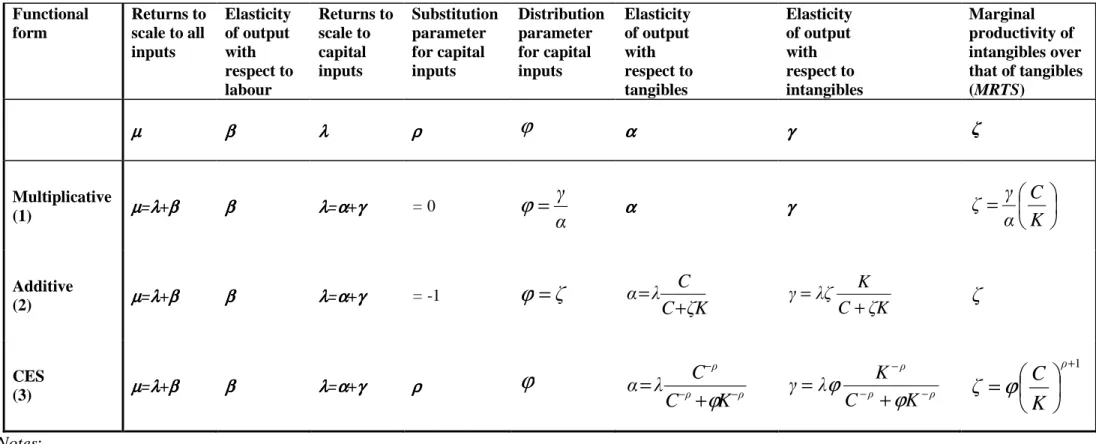
(the flexibility of response of the capital input ratio to changes in relative capital input costs) is either equals to or greater than one.

Overall, the relationships between the parameters of the three alternative production function specifications are summarised in Table 1.

Table 1 here

By taking the logarithms of equations (1)-(3), and defining all the variables per employee, the multiplicative, additive and CES production functions become, respectively:

(1') (q-l)it = ai + bt + (

µ

-1)lit +

α

(cit -lit) +

γ

(kit -lit) +

ε

mit , (2') (q-l)it = ai + bt + (

µ

-1)lit +

λ

(tcait-lit) +

ε

ait ,

(3') (q-l)it = ai + bt + (

µ

-1)lit + (

λ

/ -

ρ

) (tccit-lit) +

ε

cit ,

where lower-case letters denote logarithms;

µ

= (

λ

+

β

); in (2') tcait-lit = log[(Cit+

ζ

Kit)/Lit]; and in (3') tccit-lit = log[(Cit/Lit)-ρ+ φ(Kit/Lit)-ρ)].

In estimating the parameters of (1'), (2') and (3'), we have to face a number of empirical issues, namely: (a) the specification of the individual and temporal heterogeneity (ai and bt), and of the error terms (

ε

mit,

ε

ait,

ε

cit); (b) the non-linearity of (2') and (3') in the parameters

ζ

,

ρ

and φ; (c) the endogeneity of some explanatory variables; (d) the estimation of the MRTS in equation (1'), of the elasticity of output with respect to intangibles and tangibles in equation (2'), and of the MRTS and the elasticities in equation (3').

Issue (a) involves a number of modelling assumptions about: the non-measurable firm-specific advantages (like management ability); the influence of macroeconomic drivers (such as the business cycle, the disembodied technical change - i.e. the change over time in the rates of productivity growth); the use of common price deflators across firms (due to the usual lack of information about prices at the firm-level); the effect of imposing parameter homogeneity, whereas companies may have different production functions and rates of utilisation of various categories of input. In doing so, we assume four alternative specifications for the ai and bt parameters.

(i) Absence of individual effects (pooled OLS estimation), but the presence of industry and temporal heterogeneity that the exploratory data analysis and changes in the accounting standards suggest as relevant. This assumption is implemented by adding industry and time dummies to models' specification. If individual effects (resulting from companies’ heterogeneity in terms of their technologies, efficiency levels and use of inputs) are correlated with models' regressors, pooled estimates will be affected by omitted-variables bias.

(ii) Two-way fixed effects, both individual and temporal (within estimation). These estimates allow for additive firm-effects by using demeaned (by firm) data.

(iii) Modelling growth rates (first-differences OLS), which in the empirical models is an alternative way to allow for additive firms effects.

(iv) Modelling rates of growth over 5 years (non-overlapping long-differences or five-year differences), which is another way of estimating equations with individual effects. The advantage of long-differences over approaches (ii) and (iii) is that it preserves the cross-sectional dimension of variability. In panel data with a large N compared to T, this implies that the large variance between companies is used to identify the relevant coefficients, thus reducing the effects of other forms of misspecifications by obscuring the remaining signal in the data; see Griliches and Mairesse (1998).

Again about issue (a), we have to acknowledge that in large panels of micro data heteroscedasticity in error terms

ε

mit,

ε

ait, and

ε

cit can be substantial. In other terms, we a priori know that pure heteroscedasticity (i.e. that errors have zero-means and variances which vary by

firm i and time t) is bound to affect our inferences.2 Accordingly, we make inferences using robust standard errors with the Eicker-Huber-White estimator, see Baum, Schaffer and Stillman (2003) about its Stata implementation. This practice of making robust inferences as if heteroscedasticity was pure (i.e. independently on the presence and on the source of heroscedasticity) is discussed and motivated in Wooldridge (2002).

In order to deal with issue (b), we firstly performed grid-searches on parameters

ζ

,

ρ

and φ of the additive Cobb-Douglas and CES specifications, and obtain initial estimates by minimising equations' residual sum of squares. Then, we applied iterative procedures to first-order Taylor series approximations of equations (2') and (3') around initial values of

ζ

,

ρ

and φ which are set to the initial values obtained from the grid-searches mentioned above. Details about both grid-search and iterative procedures are provided in Appendix A1.

Issue (c) derives from a number of possible causes: the endogeneity of inputs and output in the production function; the efficiency levels - known to companies but not to the researcher - which could induce correlation between firm-effects and explanatory variables; the omission of the rates of use of labour and capital (such as working hours per employee and hours of operation per machine); other measurement errors due to e.g. changes in accounting standards and requirements, lack of information about both depreciation rates and prices at firm-level. Since we assume a one-period gestation lag before intangible and tangible stocks (K and C) become fully productive, we specify the models with beginning-of-period capital measures; in the present context, this fact has the advantage of avoiding or reducing the correlation between capital inputs and equations' disturbance terms.3 The simultaneity issue should be of less importance in the case of labour because it is measured by the average number of employees (for about half of observations).

Independently on economic endogeneity, changes in accounting legislation together with a lack of information about the different categories of workers could lead to measurement errors and so

2 _{As pointed out by a referee, there are also risks of impure heteroscedasticity, induced by specification problems such}

as not valid assumption of homogeneous slope parameter and/or omitted variables and/or incorrect functional form.

stochastic regressors. One way of dealing with endogeneity is the use of GMM estimators (see Bontempi and Mairesse, 2008). The imposition of theoretical restrictions to specific values of parameters in equations (1')-(3') is another way, easy to implement and interpret, of tackling endogeneity. This latter approach involves three steps: (s1) assuming firms' profit maximization, the labour elasticity,

β

, can be set equal to the share of labour costs in the value added; (s2) we calculate the total factor productivity (tfpc) by imposing constant returns to scale,

µ

=1; (s3) we regress total factor productivity against intangible capital, as shown in equations (1'')-(3''):

(1'') tfpcmit = ai + bt +

γ

(k-c)it +

ε

mit ,

(2'') tfpcait = ai + bt + (1-β0)(

ζ

-

ζ

(0))pKa(0)it +

ε

ait , (3'') tfpccit = ai + bt + [(1 β0)/-

ρ

](φ - φ (0))pKc(0)it +

ε

cit ,

where tfpcmit = qit –β0 lit -(1-β0)cit; tfpcait = qit – β0lit -(1-β0)tca(0)it and tca(0)it = log(Cit+

ζ

(0)Kit); tfpccit = qit – β0lit –[(1-β0)/-

ρ

]tcc(0)it and tcc(0)it = log(C-ρit + φ(0)K-ρit).

Parameter β0, labelled as slmed, is set equal to the sample median of the share of labour cost in value added (sl)4. Note that equations (2'') and (3'') above are represented as first-order Taylor-series approximations around the initial values

ζ

(0) and φ(0) (details are in Appendix A1).

Issue (d) is about the way to compute measures which depend on both parameter estimates and

the level of some variables. For example, MRTS in equation (1') may be computed as

q q K C α γ ζ       = ˆ ˆ ˆ _,

where the index q refers to three different measures of the tangibles to intangibles ratio: the 1st, 2nd and 3rd quartiles of the C/K ratio distribution.

The elasticity of output with respect to intangible capital (and similarly to tangible capital) in

equation (2') may be estimated as

γ

ˆ_q =

q K C K         +

ζ

ζ

λ

ˆ ˆ ˆ q a C T K       = ˆ ˆ ˆ

_ζ

λ

where, again, q shows that

4

We also experimented with different measures of the share of labour cost in the value-added, such as industry medians, company medians, and the Törnqvist measure 1/2∆slit. Results are robust.

we estimate three

γ

ˆ, corresponding to the 1st, 2nd and 3rd quartiles of distribution of the ratio of intangibles to estimated total capital.

The same procedure is also followed to compute the output elasticity with respect to capital inputs, and the marginal productivity of intangibles over that of tangibles in the case of equation

(3'):

γ

ˆ_q = q c q TC K K C K         =       + − − − − ˆ ˆ ˆ ˆ ˆ ˆ ˆ ˆ ˆ ˆ ρ ϕ λ ϕ ϕ λ _ρ ρ _ρ and q q K C ζ               = + 1 ˆ ˆ ˆ ρ

ϕ

.

For the CES production function the contribution to productivity of different types of intangibles can be measured in the following way. The definition of total factor productivity in this case of two different types of intangibles (e.g. intellectual versus customer capital, or capitalised versus expensed intangibles) is: tfpcdit = qit – β0lit –[(1-β0)/-

ρ

]tcdit , where d = a or b denotes the two comparisons between types of intangibles (if d = a we compare intellectual and customer capital, IK and IC; if d = b we compare capitalised and expensed intangibles, IBS and ICA). In total factor productivity formula above we have tcdit = log(TCdit) = log(C-ρit + φ1K1-ρit + φ2K2-ρit), where sub-indexes 1 and 2 indicate IK and IC for d = a and IBS and ICA for d = b; again β0, is equal to slmed, the median of the share of labour cost in value added (sl).

In this (disaggregated) context, the elasticity of output with respect to each intangibles' component and its marginal productivity with respect to that of tangibles can be estimated with the following formulae: q d q q d C T K K K C K         =         + + = − − − − − ˆ ˆ ˆ ˆ ˆ ˆ ˆ ˆ ˆ 1 1 ˆ 2 2 ˆ 1 1 ˆ ˆ 1 1 1 ρ

ϕ

λ

ϕ

ϕ

ϕ

λ

γ

_{ρ ρ}ρ _ρ and q q d

K

C

ζ





























=

+1 ˆ 1 1 1

ˆ

ˆ

ρ

ϕ

which combines the estimates of the total factor productivity equation with the 1st, 2nd and 3rd quartiles q of the sample distribution of relevant capital ratios data, and where 1 = IK and 2 = IC for d = a and 1 =IBS and 2 =ICA for d = b;

γ

ˆd2q and

ζ

ˆ

d2q are obtained similarly.

3. Data sources and measurement issues

The estimation of the theoretical models listed above is based on a dataset of company data for the variables Q, L, C, and K. Our dataset is constructed from three sources: the Company Accounts Data Service (CADS) for the financial reporting information, the National Accounts data (NA) of the Italian National Institute for Statistics (ISTAT) for depreciation rates and deflators, and the Survey on Investment in Manufacturing Firms (SIM) conducted annually by the Bank of Italy for the purpose of selecting sub-samples according to the presence of spillovers (see Section 5).

The main data source is CADS provided by Centrale dei Bilanci, a company – set up jointly by the Bank of Italy andthe ABI (Italian Banking Association) and other leading Italian banks – which has been collecting firm-level data since 1982. CADS is a large database with detailed accounting information from more than 148,000 Italian companies operating in a wide range of industrial and service sectors. CADS is highly representative of the population of Italian firms, covering over 50% of the value added by those companies included in the Italian Central Statistical Office’s Census. Further details of this dataset can be found in Bontempi (2011).

Appendix A2.1 describes the cleaning rules applied to the original CADS dataset. The final sample we selected is an unbalanced panel of 14,254 Italian manufacturing firms with an average of 6.7 years over the 1982-1999 period (94,968 observations).

3.1. The measurement of tangible and intangible capital: the information provided by company accounts

Table 2 shows how we used accounting items in order to define tangible (Panel A) and intangible (Panel B) capital stocks. Each cell of Table 2 contains details of the accounting categories of tangibles and intangibles available in our dataset.

Table 2 here

Panel A illustrates our definition of tangible stock. As with intangibles, the cells show the six tangible assets, from (T1) to (T6), enumerated by the Italian GAAP. We label these categories TBSr,

where r=bui, pla, equ, oth, unc, lea. Our definition of total tangible capital is C=

∑

r r

TBS , where r=bui (buildings), pla (plants), and equ (equipment). We therefore excluded leasing (r=lea) as it is essentially insignificant, and dismissed and uncompleted tangibles (r=oth, unc) because of their not-yet and/or no-longer productive nature.5

Panel B of Table 2, which focuses on intangibles, merits further explanation because it has to do with the debate on whether and which category of intangibles it would be better to capitalise or to expense. These questions are the most controversial issues that have recently been raised in the literature on the topic. From the microeconomic point of view, mention should be made of the debate faced by the International Accounting Standards Committee (IASC) when developing the International Financial Reporting Standards (IFRS - International Accounting Standards, IAS, until 2002) designed to be universally adopted. Improving accounting for intangibles is one of the major challenges for future financial reporting because the asymmetric way of dealing with tangible resources – treated as investments – and intangible resources - treated as costs – is believed to have increasingly reduced the value-relevance of financial reporting (Høegh-Krohn and Knivsflå 2000). Microeconomic analysis of this issue is provided by the works of Lev (see, e.g., Lev, 2001). Yet the debate is of interest from the macroeconomic point of view, too: firms’ expenditures in knowledge creation until now have largely been excluded from national accounts (GDP) and capital stock, and uncounted intangibles have a significantly negative effect on the measured pattern of economic growth. For this reason, one of the major changes in defining the new System of National Accounts (SNA) regards the recognition of non-ICT intangibles: innovative property such as R&D, design and product development in financial services, and economic competencies such as market research, advertising, training and organisational capital; see the literature, starting from Corrado et al. (2005 and 2009).6

5

When we use the broader definition of tangibles, estimation results do not change significantly. All non-reported results of the present paper are available upon request.

6 _{Software, mineral explorations and entertainment and artistic originals are the only components that are considered}

In Italy the reporting of intangibles is subject to a combination of national GAAP7 and IAS 38 plus IFRS 3 standards (which supersede IAS 22). This combination implies that, notwithstanding the fact that the criteria employed in recognising intangible assets are similar to those of the IAS/IFRS,8 this combination accounts for more intangible assets than those provided for by IAS/IFRS. In fact, Italian GAAP present a specific list of intangibles that should be capitalised, i.e. recorded as assets in the balance sheet: (I1) start-up and expansion expenses; (I2) research, development and advertising costs; (I3) patents and intellectual property rights; (I4) concessions, licences, trademarks and similar rights; (I5) goodwill; (I6) assets being evaluated and payments on accounts related to intangible assets; (I7) others. Italian GAAP also require that certain other specific intangibles (or those intangibles that do not qualify for capitalisation as assets) are recognised as costs when incurred. Hence, deferred charges – such as development costs, advertising and applied research spending – and items such as brands are intangibles capitalised as assets and thus treated as valuable investments by Italian GAAP. In contrast, the criteria for recognition of an intangible asset applied by IAS/IFRS and based on the prudence principle imply that resources spent on such items can only be expended and thus reported as costs.9 The justification at the basis of IAS/IFRS is the uncertain, discontinuous nature of many intangibles: the amount of intangibles to be capitalised would be too subjective, thus offering managers a means by which to manipulate reported earnings and asset values.

It could be argued, however, that the level of uncertainty of specific intangibles is not notably higher than the uncertainty of other corporate investments, such as stocks or bonds. The expensing

7 _{Based on article 2424 of the Italian Civil Code, on Legislative Decree no. 127/91 implementing the Fourth European}

Commission Directive which modified a number of accounting standards, and on principle no. 24 of the Commissione

per la Statuizione dei Principi Contabili of the Consiglio Nazionale dei Dottori Commercialisti e Ragionieri.

8 _{An intangible asset should be recognized at cost if and only if it is identifiable, it is probable that specifically}

attributable economic benefits will flow from the assets, and its cost can be measured reliably.

9

Intangibles initially recognized as an expense should not be recognized as part of the cost of an intangible asset at a later date.

of intangibles also affords managers a powerful manipulation tool which is arguably more damaging than manipulation-via-capitalisation. The disparity of treatment between intangible and tangible assets could make short-term behaviour attractive to managers; furthermore, it could mislead investors relying upon the financial statement as their primary source of information. Several descriptive studies, in fact, document that not recognising intangibles as assets hampers the value-relevance of financial statements (among others, Aboody and Lev, 1998, regarding software development costs). Statistical evidence also suggests that the capitalised value of intangibles, such as R&D costs, would provide important information to investors when they are pricing securities (Lev and Sougiannis, 1996, and Hulten and Hao, 2008).

In Table 2, Panel B, the categories from (I1) to (I7) represent the intangibles which, according to Italian GAAP, are capitalised; we have labelled these categories IBSj (j=start, rd, pat, mark, god, fin) to indicate intangible capital stock reported in the balance sheets. For the sake of consistency, we created categories (I8)-(I10) to indicate intangibles that cannot be capitalised, but only expensed; in these cases, the intangible capital stocks are computed from the costs, DEh (h=rd, pat, adv), reported in current accounts, according to the PIM described in Appendix A2.2. We have labelled these intangibles ICAh (h=rd, pat, adv).

The Italian case thus makes it possible to lighten the effect of both capitalised and expensed intangibles on company productivity. In other terms, the treating intangibles as assets for accounting purposes exploits inside information about depreciation/obsolescence and expectations concerning future profits on the part of managers; these settlements are unknown to the econometrician and can be compared with assumptions about the starting values, the depreciation rates and the negligibility of disinvestment/scrapping he makes when implementing the PIM formula.

We can also disentangle the effect on productivity of the different natures of intangibles: those having to do with research, development, information and communication technology, which we call intellectual capital, IK, and those exploiting and improving relationships of a company with its

customers, which we call customer capital, CK. Of course, we can also assess which of the two types – intellectual or customer –is mainly composed of capitalised or expensed intangibles.

Hence, we define total intangible capital (K) in two different ways.

(1) Focusing on the different accounting treatment, we define K = IBS + ICA (along the rows of Table 2, Panel B). Intangibles capitalised as assets and thus treated as valuable investments are

∑

= _j j

IBS

IBS with j=rd (applied research and development costs, advertising costs which are

functional and essential to the start-up phase), pat (purchased and internally-developed patents, software and intellectual property rights), and mark (purchased and internally-developed trademarks, concessions, licences and similar rights). Intangibles expensed, and thus reported as costs, are ICA=

∑

h h

ICA

with h=rd (basic research), pat (regular licence fees paid for patents), and adv (operative and recurrent advertising).

(2) Focusing on the economic nature of intangibles, we also define K = IK + CK (along the columns of Table 2, panel B). Intellectual capital is IK=

∑

_jIBS +j

∑

h h

ICA

, with j=rd, pat and h=rd, pat; it is composed of R&D and patents regardless of whether they are capitalised or expensed. Customer capital is CK=

IBS

j

+

ICA

h, with j=mark and h=adv; it consists of trademarks (capitalised) and advertising (expensed).

The last column in Table 2, Panel B, shows the accounting information on other intangibles which is available to us in the balance sheets. Formation/expansion/start-up expenses (start) and goodwill (good) have not been taken into consideration, given their miscellaneous or peculiar natures, which require further, specific analysis.10 Deferred financial charges (fin) have to be excluded from the analysis of company productivity; finally the category (I6), given its specific nature, has been reallocated to other categories, from (I1) to (I5).11

10_{The results are assessed in terms of whether they are robust enough to “start-up” to the inclusion of the start category.} 11 _{The reallocation procedures also take into account the legislative changes introduced in 1992, when the fourth}

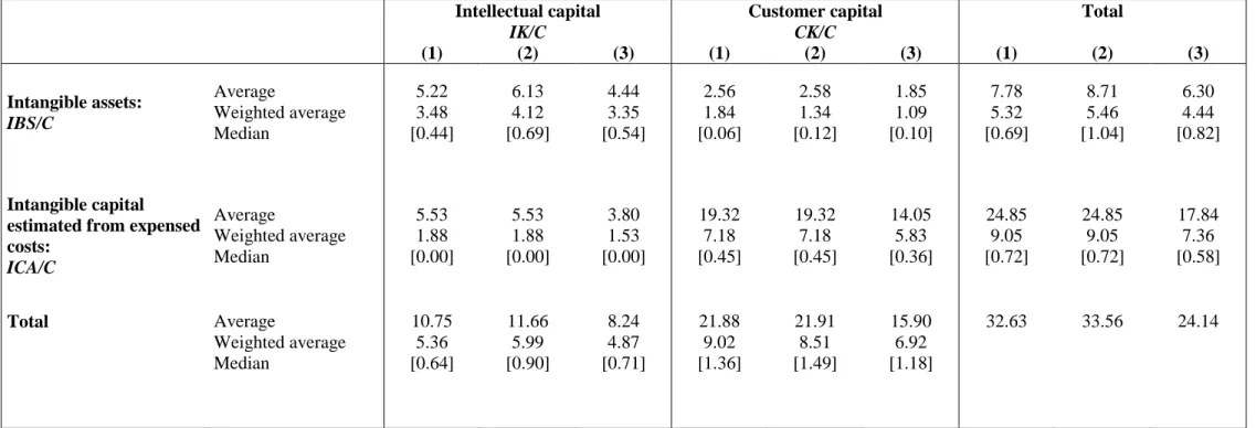
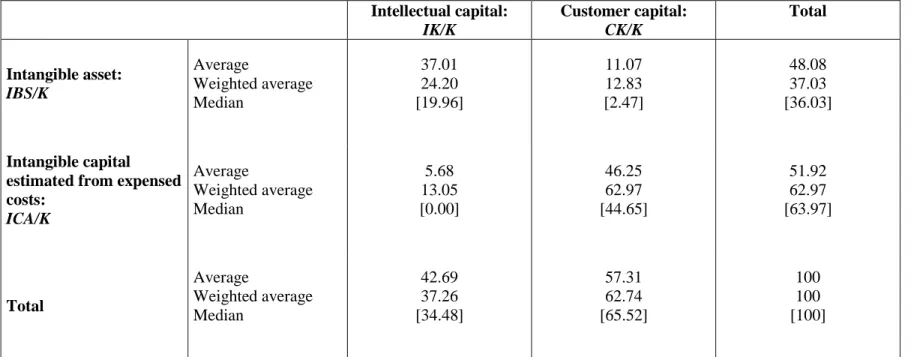
3.2. Intangible capital components: occurrence and magnitude compared with tangible capital In this section we analyse the magnitude and occurrence of intangible capital and its components. Each cell of Tables 3 and 4 shows the mean (in the first row), the weighted average (in the second row) and the median (in squared brackets, third row) of the ratio of intangibles to tangibles (in Table 3) and of the percentage composition of total intangible capital (in Table 4). The figures in Table 3 refer to: the book values of both intangible and tangible assets (in columns (1)); the replacement values for intangible assets and the book values of tangible assets (in columns (2)); the replacement values of both intangible and tangible assets (in columns (3)). Replacement values are obtained by applying the PIM; of course, stocks computed from expensed intangibles are always at replacement values (see Appendix A.2.2). The comparison of assets at both book and replacement values with intangible capital computed from expensed intangible costs makes it possible to evaluate the effect of estimating stocks instead of using assets as they are reported in the balance sheets. Since results are robust to the use of different measures (book or replacement values) of capitalised intangibles (and tangibles), in Table 4 both intangible and tangible assets are at book values, as in columns (1) of Table 3.12

Table 3 and 4 here

Distinguishing between the different types of intangibles,

ICA

adv (the part of customer capital

relating to operative and recurrent advertising costs) and

∑

j j

IBS with j=rd, pat (the component of intellectual capital due to applied R&D, patents, software and intellectual property rights) are the first and second most important intangibles, regardless of the scale attributed to the phenomenon (total tangibles or total intangibles). The component of customer capital capitalised by firms,

mark

IBS

(trademarks, concessions, licences and similar rights) and the part of intellectual capital

illustrates the procedures we followed in order to link the reporting rules of Italian GAAP with the accounting information available for our sample of Italian companies, and the empirical variables suitable for productivity analysis.

computed from basic research costs and licence fees paid for patents,

∑

h h

ICA

with h=rd, pat , follow in third and fourth positions respectively.

Intangible capital and its components are further analysed by taking into account the role of values equal to zero.13 The results are reported in Table 5, for total manufacturing (in bold) and for the sub-samples of manufacturing according to their global technological intensity.

Table 5 here

To make comparison easier, the first row, labelled “Full sample Total”, shows the same results as those given in Table 3, columns (1). The upper part of Table 5 reveals how the average intangible-to-tangible ratios change in the sub-samples in which total intangible capital and the two combinations of its components are never equal to zero. The percentage of observations featuring zero intangibles is not relevant (about 17%), as is clear if we compare the numbers of observations in the “Full sample Total” and the “K never zero Total” rows.

The “Both IK and CK never zero Total” and “Both IBS and ICA never zero Total” observations represent 64% and 35%, respectively, of the “K never zero Total” sample. Advertising expenses are rarely characterised by continuous initial zeros; hence, the stock

ICA

advcomputed by the PIM,

which is the main component of CK, is almost unaffected by zeros. In contrast, the rare presence of initial non-zero observations in R&D and patent expenses affects the corresponding stocks, included in ICA.

Given the definition of intangible capital presented in Table 2, the comparison of the percentages reported in the “IK never zero (and CK zero) Total” row shows that intellectual capital is mainly composed of applied R&D and patents (77%), which are recognised as an asset and thus included in IBS. Basic research and patent royalties (expensed out and included in the ICA component) represent only 23% of IK (and are an almost negligible component of ICA). In contrast,

13

At the parameter-estimation stage, we used two approaches: focusing on the sub-sample of K never equal to zero; using the full sample and including specific dummy variables indicating observations with null values for intangibles. The results are quite robust, especially, as expected, in the additive and CES specifications, equations (2) and (3).

operative and recurrent advertising costs (in ICA) are the main component of CK (88%); this is shown by the “CK never zero (and IK zero) Total” row of Table 5. Trademarks account for just 12% of customer capital: see the combination of “CK never zero (and IK zero) Total” row with the IBS column.

The “Full sample” rows disaggregated according to the technological intensity of industries and the “K” column of Table 5 display a high value for the ratio of total intangible capital (K) to total tangible capital (C) in the LT industry. This result can be explained by looking at the other columns on the right-hand side of Table 5: it is clearly driven by the component consisting of expensed intangibles (ICA) and, in particular, of customer capital (CK). Advertising and trademarks are also important to the HT+HMT industry; nevertheless, as we expected, applied R&D and patents (included in the IBS category) played an important role compared to other branches. These results are confirmed by the disaggregation by industries of the “K never zero” row, and are further emphasised by the “IK never zero (and CK zero)”, “CK never zero (and IK zero)”, “IBS never zero (and ICA zero)” and “ICA never zero (and IBS zero)” rows.

3.3. Basic descriptive statistics of the models’ variables

The main statistics of the variables of interest are reported along the columns of Table 6. Table 6 here

Per-employee level statistics, measured in millions of Italian Lira at 1995 prices (in the upper part of Table 6), suggest considerable departures from normality: means are always bigger than the corresponding medians; the effect of outliers in causing departures between parametric and non-parametric measures of spread (standard deviation, SD, and inter-quartile range, IQR) is evident; these results particularly characterise the number of employees and intangibles. Of all of the variables, intangibles represent the most extreme cases: for example, the parametric measures of centre and spread of the total intangible stock per-employee are about five times bigger than the corresponding non-parametric measures (in particular, the mean is well over the 3rd quartile). The same features are largely reproduced by the intangible-to-tangible ratio because of intangibles as the

numerator. These facts suggest that large intangible stocks are concentrated in relatively few companies, and that zeros are more prevalent here than for the other variables.14

The distribution of labour costs seems almost normal, with variability that is less than one-third of the average. In other terms, the share is quite well summarised by the measures of centre of the distribution; the labour share of value added averages at about 65% of production.15

As far as growth rates are concerned (in the lower part of Table 6), per-capita production figures, value added, intermediate inputs, and, to a lesser extent, tangible stock statistics are similar to each other over the sample period. Employment growth is slightly more stable than previous productivity measures, while statistics for total intangibles suggest a 30-50% higher variability than previous variables. Variability of intangibles is emphasised when disaggregated components are considered, mainly due to the larger presence of zeros, as shown by the reduced number of observations and companies involved in the computations of growth rates (the numbers for NT and N, respectively, reported in the notes to Table 6). This variability is reduced when measured by robust statistics.

Table 6 also presents the total variability decomposition in between (i.e. across) firms and within firms (i.e. due to time). Variables measured in levels have a between-firm variability that is always greater than 70-80% of the total variability, the only exception being the labour cost share. Between-firm variability greatly loses its relevance when growth rates are considered and level information is lost: sample variability due to individual effects drops to about 15-20%. The higher between-firm variability for the intangible stock growth rate confirms the significance of a few individual companies, as outlined above. In general, time never exhibits a significant role in explaining variability; this result, in line with the findings of other studies (see, among others, Griliches and Mairesse, 1984), must be taken into consideration when interpreting estimation results. The main features illustrated in Table 6 for the whole sample are qualitatively the same if

14 _{These facts suggest the use of the 1}st_{, 2}nd _{and 3}rd _{quartiles in computing MRTS in the multiplicative specification, and}

the elasticity of output with respect to intangibles in the additive specification.

we split the sample into the three sub-samples corresponding to the high-, medium- and low-technology sectors (see Bontempi and Mairesse, 2008, Table A1).

Regarding the correlation matrix between the variables, we note that levels only occasionally record simple correlations in absolute values which are in the 0.2-0.4 range, while in differences the correlations are hardly ever larger than 0.2. Therefore, we can be confident that multicollinearity is not an issue in estimating the models listed in Section 2. This is quite usual in large panels of micro-data.

4. Baseline results using aggregate intangibles

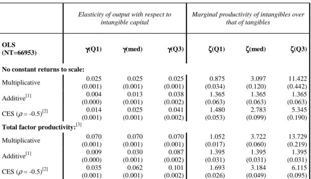
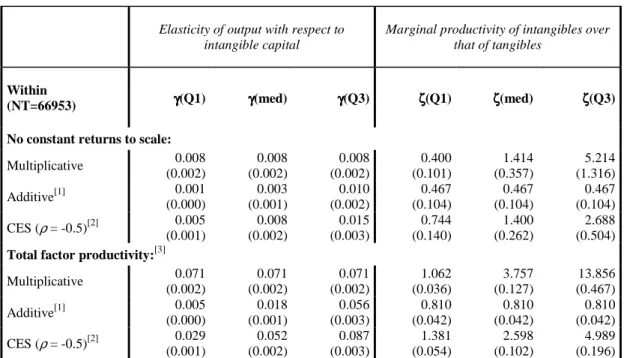
We report in the four Tables 7a-7d the estimation results of the cases listed in Section 2 by using aggregate intangible data described in Section 3 as a measure for K. In particular, each table reports decreasing restrictive assumptions regarding parameter heterogeneity, going respectively from Table 7a (reporting the pooled estimates, where the assumption of heterogeneity is minimal) to Table 7d (reporting five-year-long differences). Each table has the same structure: two blocks of three lines reporting estimation results that respectively come from multiplicative and additive Cobb-Douglas and CES models. This three-line block is repeated two times in each table because we report both the estimates from the least restricted parameters of equations (1')-(3'), i.e. no constant returns to scale, and those for the most restricted parameters of equations (1'')-(3''), i.e. total factor productivity (these restrictions are discussed in Section 2).

Tables 7a-d here

The column structure of Tables 7a-7d is the same. The first three columns report the estimates of the elasticity of output with respect to intangible capital (which is constant and directly estimated in the multiplicative Cobb-Douglas, and computed by combining parameter estimates with quartiles of data sample distribution in the additive Cobb-Douglas and CES). The last three columns report the estimates of the marginal productivity of intangibles over that of tangibles (which is constant

and directly estimated in the additive Cobb-Douglas, and computed by combining parameter estimates with quartiles in the multiplicative Cobb-Douglas and in CES).16

The constant elasticity, as directly estimated by the multiplicative Cobb-Douglas, is similar to elasticity as estimated in correspondence to the third quartile by the additive Cobb-Douglas, and to the second quartile by CES, given the distribution of the ratio of intangibles over estimated total capital. Symmetrically, MRTS, which is directly estimated by the additive Cobb-Douglas, is similar to those obtained from the estimates of the multiplicative Cobb-Douglas and CES in correspondence to the first quartile of the distribution of the tangibles/intangibles ratio. These results reflect the patterns reported in Table 6, from which it emerges that the distribution of intangibles over tangibles is positively skewed because intangibles are much more highly concentrated within a small number of companies.

Overall, aggregate intangibles K always play a significant role in explaining productivity. This fact is robust to heterogeneity assumptions (i.e. to the estimation method) in terms of both elasticity and marginal productivity over tangibles. It is also worth noting that the total factor productivity equation (3'') in the lower blocks of Table 7a-7d always delivers significantly larger estimates than those produced by the non-constant returns to scale equation (3) in the higher blocks. Given that endogeneity in this context is expected to induce negative biases of estimates, this fact suggests that, as shown in Section 2, the total factor productivity restriction is able to deal with endogeneity (GMM estimates, not reported here but available in Bontempi and Mairesse, 2008, Table 9, support this finding).

Given the parameter estimates of different models with alternative estimators, it may be interesting to inspect how wide the intervals are between the third and the first quartile of the marginal productivity of intangibles over tangibles reported in Table7a-d. The width of these inter-quartile intervals depends on the way in which point estimates of

γ

,

α

, and

ϕ

parameters interact

16 _{See Table 1 for the summary of the relationships between model parameters, specific capital ratios, elasticity and}

with the sample distribution of the ratios of tangible over intangible capital. The larger parameter estimates under the assumption of valid total factor productivity explain the wider intervals compared to the non-constant returns to scale specification. Overall, independently of the theoretical model and the estimation method, all of the ranges broadly overlap the range of CES estimated with long differences which, in this way, can be taken as representative of the overall results. This range of marginal productivity of intangibles over tangibles is between one and four, and suggests that the advantage in terms of productivity given by intangible capital is more than four times the productivity gains of tangible capital for more than one quarter of the firms in our sample. At worst, for another quarter of the firms, such relative productivity is slightly larger than one (again, in favour of intangibles).

If we focus on the estimates corresponding to the sample medians (MED), the within and five year-difference estimates appear somewhat similar, confirming the relevance of accounting for heterogeneity. Regarding the models, CES specification can be seen as a reasonable compromise between the point estimate of the additive Cobb-Douglas and the large range of values of the multiplicative Cobb-Douglas.

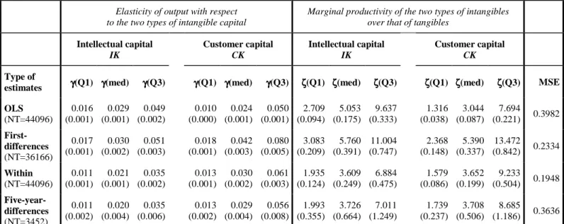
5. Results using different types of intangible assets

On the basis of the theoretical framework depicted in Section 2, and using the estimation method outlined in Appendix A1, in this section we report the estimates of the parameters of a CES production function which embodies total factor productivity restrictions (to deal with the endogeneity issue) and we evaluate the contribution to productivity of different types of intangibles.17_{In particular, Table 8a reports the results by splitting total intangibles into intellectual}

capital IK, and customer capital CK.18 Table 8b reports the results by splitting total intangibles into intangible assets, IBS, and intangibles capitalised from expenditures, ICA.

17 _{Estimates obtained by using other specifications of the production function are available upon request.}

18 _{The IK variable includes IT and telecommunications, engineering and design, R&D-related services, filings for}

Table 8a and 8b here

In Table 8a, the differences between the estimated marginal productivities of IK and of CK tend to be concentrated in the third quartile, and become less relevant as we move from OLS and first-differences to within and long-difference estimation methods. Conversely, the differences between the estimated marginal productivities of IBS and of ICA in Table 8b are always quite important, independently of the estimation method used. In addition, within and five-years differences estimates are smaller than those obtained from OLS and first-difference methods. In general, the pattern of estimates from the estimation method confirmed what was previously found at the aggregate level (see Section 4).

If we define as a reference for our results the aggregated intangible estimates obtained by long differences applied to the total factor productivity specification of the CES production function (the results of which are reported in the last row of Table 7d), ICA displays a marginal productivity in line with that of total intangibles, and its marginal productivity is smaller than that of IBS, of intellectual capital, IK, and of customer capital, CK, (which is the highest).

Italian GAAP leave managers free to some extent in deciding whether or not to capitalise R&D. Albeit based on a priori and subjective expectations on uncertain profits, the choice of capitalising some intangibles by managers seems to increase the value relevance of financial reporting: capitalised intangibles are those which drive firms’ performance most strongly. In other terms, IBS exploits managers’ inside information about the economic benefits expected to flow from resources spent on intangibles and, as such, offers a measure of knowledge capital which is more reliable than the one computed by the econometrician on the basis of a limited information set. This result is in line with the findings of Høegh-Krohn and Knivsflå (2000) and Zhao (2002) who compare Scandinavia, the UK, France (capitalising countries) with Germany and the USA (expensing countries): the value relevance of financial statements would be improved if expensed

organizational and operational innovation or product innovation, while the CK variable includes marketing, advertising, promotions, market research, and trademarks.

costs in knowledge, design, licences, and trademarks were partly capitalised. Moreover, the allocation of R&D costs between capitalisation and expense further increases the value relevance of R&D reporting in France and the UK.

By comparing Tables 8a and 8b, IK and IBS estimates are very close because intellectual capital mainly consists of intangible assets (see Table 2). This is no longer true if we compare CK and ICA, as customer capital has larger estimates than those of intangibles capitalised from expenses. This result suggests that ICA productivity is mainly driven by advertising, rather than by basic R&D and patent royalties.19 Finally, it should also be noted that trademarks and brands (i.e. the portion of CK made of intangible assets) play a significant role in raising the productivity of customer capital over that of tangibles. Greenhalgh and Rogers (2012) find that UK firms that trade mark are characterised by significantly higher value added than non-trademarkers.

Until now we have focused on the empirical examination of the influence of intangibles (and their composition) on productivity at the firm level. However, a important feature of intangible assets is that their social value is substantially larger than the portion that is captured by estimates based on firm data. In order to extend our results to aspects coming from the spillover (or network) literature on intangibles, we selected some sub-samples of the whole dataset in which we estimate the same relationships described above. In this way, we were able to assess – through parameter changes – the extent to which the role of intellectual (IK) and customer (IC) capital increases if measured in contexts where the externalities are expected to increase the effect of intangibles on productivity. Our results are reported in Table 8c.

Table 8c here

Before analysing the results in sub-samples, it should be noted that the definition of the sample-selection (binary) variables requires that the “old” (CADS-based) dataset is merged with SIM, the annual survey conducted by the Bank of Italy which provides additional information on

19 _{Estimates of the productivity of total intangibles computed by excluding advertising show results qualitatively similar}