Diversification and Ownership Concentration

D

S

E

Working

Paper

Dipartimento

Scienze Economiche

Department

of Economics

Ca’ Foscari

University of

Venice

Diversification

and Ownership

Concentratio

Loriana Pelizzon

Bruno Parigi

W o r k i n g P a p e r s D e p a r t m e n t o f E c o n o m i c s C a ’ F o s c a r i U n i v e r s i t y o f V e n i c e N o . 2 9 / W P / 2 0 0 7 ISSN 1827-336X T h e W o r k i n g P a p e r S e r i e s i s a v a i l b l e o n l y o n l i n e ( w w w . d s e . u n i v e . i t / p u b b l i c a z i o n i ) F o r e d i t o r i a l c o r r e s p o n d e n c e , p l e a s e c o n t a c t : w p . d s e @ u n i v e . i t D e p a r t m e n t o f E c o n o m i c s C a ’ F o s c a r i U n i v e r s i t y o f V e n i c e C a n n a r e g i o 8 7 3 , F o n d a m e n t a S a n G i o b b e 3 0 1 2 1 V e n i c e I t a l y F a x : + + 3 9 0 4 1 2 3 4 9 2 1 0

Diversification and Ownership Concentration Loriana Pelizzon

University of Venice and SSAV

Bruno Parigi University of U n i v e r s i t y o f P a d u a , a n d C E S i f o . Abstract I n a m e a n - v a r i a n c e e c o n o m y w h e r e c o n t r o l l i n g s h a r e h o l d e r s c a n d i v e r t p r o f i t s , e q u i t y o w n e r s h i p i s m o r e c o n c e n t r a t e d t h e h i g h e r t h e s t o c k r e t u r n s c o r r e l a t i o n . A h i g h e r r e t u r n s c o r r e l a t i o n r e d u c e s t h e b e n e f i t s o f d i v e r s i f i c a t i o n , g i v i n g r i s e t o b o t h a h i g h e r i n v e s t m e n t b y t h e c o n t r o l l i n g s h a r e h o l d e r i n t h e a s s e t t h a t h e c o n t r o l s a n d a l o w e r i n v e s t m e n t b y t h e n o n - c o n t r o l l i n g s h a r e h o l d e r s . T h e e m p i r i c a l a n a l y s i s s u p p o r t s t h e p r e d i c t i o n s o f t h e m o d e l . I n p a r t i c u l a r , c o n t r o l l i n g f o r m e a s u r e s o f t h e q u a l i t y o f i n v e s t o r p r o t e c t i o n , a n d o t h e r s t r u c t u r a l v a r i a b l e s , w e f i n d t h a t e q u i t y o w n e r s h i p i s s i g n i f i c a n t l y m o r e c o n c e n t r a t e d i n c o u n t r i e s w h e r e t h e s t o c k r e t u r n s c o r r e l a t i o n i s h i g h e r . M o r e o v e r t h e i n t e n s i t y o f t h e r e l a t i o n s h i p b e t w e e n t h e s t o c k r e t u r n s c o r r e l a t i o n a n d o w n e r s h i p c o n c e n t r a t i o n i s a m p l i f i e d b y p o o r i n v e s t o r p r o t e c t i o n . Keywords Ownershipconcentration,Diversificationopportunities,Investor protection. JEL Codes D8,G2,G3

Address for correspondence:

Loriana Pelizzon Department of Economics Ca’ Foscari University of Venice Cannaregio 873, Fondamenta S.Giobbe 30121 Venezia - Italy Phone: (++39) 041 2349164 Fax: (++39) 041 2349176 e-mail: [email protected]

This Working Paper is published under the auspices of the Department of Economics of the Ca’ Foscari University of Venice. Opinions expressed herein are those of the authors and not those of the Department. The Working Paper series is designed to divulge preliminary or incomplete work, circulated to favour discussion and comments. Citation of this paper should consider its provisional character.

Diversi

fi

cation and ownership concentration

November 11, 2007

Abstract

In a mean-variance economy where controlling shareholders can divert profits,

equity ownership is more concentrated the higher the stock returns correlation. A higher returns correlation reduces the benefits of diversification, giving rise to both a higher investment by the controlling shareholder in the asset that he controls and a lower investment by the non-controlling shareholders. The empirical analysis supports the predictions of the model. In particular, controlling for measures of

the quality of investor protection, and other structural variables, we find that

equity ownership is significantly more concentrated in countries where the stock

returns correlation is higher. Moreover the intensity of the relationship between

the stock returns correlation and ownership concentration is amplified by poor

investor protection.

Key words: Ownership concentration, Diversification opportunities, Investor protection.

1. Introduction

Recent research reveals a number of differences among countries with respect to own-ership structure, portfolio allocation, and stock market participation. One strand of literature argues that these differences are shaped by the extent of legal protection for outside shareholders (La Porta et al. 1997, Kumar et al. 1999, La Porta et al. 1999, Nenova 2003, among others). Poor investor protection allows controlling shareholders to extract benefits from the companies that they run (La Porta et al. 2000), and the presence of control benefits is the most common explanation for ownership concentra-tion and the resulting loss of diversification (Zingales 1994, Demsetz and Lehn 1985). A number of empirical studies show that ownership is more concentrated in countries with poorer investor protection (see for example La Porta et al. 1998).

The objective of this paper is to contribute to understanding of the differences in own-ership concentration around the world by pointing out a missing link between ownown-ership concentration and shareholder protection: diversification opportunities affect ownership concentration when investor protection is poor.

We consider a mean-variance general equilibrium economy with one risk-free asset and several risky assets that can be interpreted as “firms”.1 _{Some investors, the} “house-holds", have no control over anyfirm, whereas others, the “entrepreneurs”, have control over their own firms. Controlling shareholders obtain higher expected returns than do non-controlling shareholders because they are able to divert a fraction of the profits from the firm that they control. Since the returns on the risky assets are imperfectly correlated, there are benefits from portfolio diversification. The portfolio decisions of all

1_{Theoretical work in this area is only starting to develop. Most existing models, though, are} con-structed in a partial equilibrium framework with risk-neutral agents (La Porta et al. 1998, 1999, Zin-gales 1995, Bennedsen and Wolfenzon 2000). An exception is the general equilibrium study by Shleifer and Wolfenzon (2002), which in a risk-neutral environment examines the impact of the endogenously determined level of investor protection on the ownership structure offirms that go public.

individuals - households and entrepreneurs - generate a demand for shares of the assets. The model determines the fraction of the wealth invested in the risk-free asset and in the risky assets and, as a result, thefirms’ ownership structure. We show that diversification opportunities, which we measure as the stock returns correlation in a given economy -the “local market correlation” - matter in explaining portfolio allocation and ownership structure.

The theoretical model yields several insights. First, profit diversion induces control-ling shareholders to hold less diversified portfolios. A higher level of profit diversion makes controlling shareholders retain both a larger share of the assets that they control, and a smaller share of the other risky assets than would be required without profit diver-sion. The first part of this result is well known in the literature: for example, Zingales (1994) observes that there is little reason to hold a large block of shares unless there are benefits of control. However, low portfolio diversification may also arise because of a second effect that we can capture through our general equilibrium model: the pres-ence of control rights induces a lower investment in the risky assets controlled by other entrepreneurs. This theoretical result is consistent with the stylized fact noted by La Porta et al. (1999) that in general there is no other large shareholder to monitor the controlling shareholder.

Second, the general equilibrium nature of our model allows us to assess the im-pact of diversification opportunities on ownership concentration, which we define as the fraction of the shares of a firm held by the controlling shareholder with respect to the shares of the samefirm held by other entrepreneurs. Ownership concentration increases when diversification opportunities decline because, other things being equal, each con-trolling shareholder invests a larger share of his wealth in the assets that he controls.

Similarly, when diversification opportunities decline, non-controlling investors allocate a lower fraction of their wealth to the risky assets that they do not control.

Third, the impact of the stock returns correlation on ownership concentration is am-plified by poor investor protection. The reason is that the poorer the investor protection, the lower the cost of sacrificing diversification, so that poor investor protection reinforces stock returns correlation in making it more attractive for controlling shareholders to in-vest in the assets that they control.

We then take the model to the data and investigate whether diversification oppor-tunities matter in explaining ownership concentration. Our main empirical finding is the novel one that ownership is more concentrated in countries where stock return cor-relations are higher. Second, poor governance amplifies the impact of the stock returns correlation on ownership concentration. Third, the ability to obtain control benefits with a small ownership stake because of pyramids weakens the impact of stock return correlations on ownership concentration. Finally, our results suggest that local market correlation is a relevant variable in explaining ownership concentration even if we allow for international diversification.

One may argue that the positive relationship between ownership concentration and stock returns correlation is spurious. A first set of objections concern the possibility that control benefits and public risk-return profiles both depend on the strength of institutions, and this may have biased our empirical analysis. We addressed this issue by using two-stage least squares regressions to disentangle the impact of stock returns correlation from the quality of institutions on ownership concentration. This analysis suggests that one of the channels through which the strength of institutions affects ownership concentration is indeed diversification opportunities.

A second criticism concerns the possible presence of reverse causality: ownership concentration may affect stock returns correlations, which therefore may be endogenous. To investigate the evidence against the exogeneity of stock returns correlations we per-form a Hausman (1978) test whose results reject the hypothesis of endogeneity of stock returns correlations.

The rest of the paper is organized as follows. Section 2 presents the model. In Section 3 we derive the optimal portfolio, the equilibrium ownership structure, and the comparative static results w.r.t. stock returns correlations. Section 4 tests the empirical relevance of our results. Section 5 discusses some extensions and concludes.

2. Model

Consider a two-period economy withn+ 1 assets; assets 1, .., nare risky, asset n+ 1 is safe. Denote with Ii the investment in asset i. All risky assets have the same expected gross returns per unit, mi = m. The gross return from investment in risky assets i is

˜

R(Ii) = (m+ i)Ii, where i is a random variable with E( i) = 0, E( i j) = σij >

0, i ₆= j. All risky assets have the same standard deviations, σi = σ, and correlation coefficients between their returns,ρ_ij =ρ, i₆=j = 1, ..., n. It follows that the correlation coefficientρis greater than zero, so that risk cannot be completely eliminated from any portfolio. We assume that ρ <1, i.e. there are diversification opportunities. The rate of return on the risk-free asset is normalized to zero; that is, R˜n+1(In+1) =In+1.

There aren+ 1individuals. Individuals1, ..., nare “entrepreneurs”. Individualn+ 1

represents the "households" sector, which we will consider as a unique representative agent. Each individual is endowed with Wj > 0 units of consumption good; the total endowment isW =Pn+1_j=1 Wj units of consumption good.

Entrepreneur i “controls” risky asseti, and only that asset. In turn, a risky asset is controlled by only one entrepreneur. Which individuals are entrepreneurs and which is the household, and which asset an entrepreneur controls, are exogenously determined. Control allows entrepreneur i to divert an amount B(Ii) of the profits realized by the asset that he controls. Following La Porta et al. (1998) we assume that the effective amount of profit diversion is the result of the interactions of many factors, among which are the rules that protect outside investors and the quality of the enforcement of these rules. There is ample empirical evidence that the scope for profit diversion grows with

firm size. For the sake of simplicity we assume that profit diversion is the same proportion of investment for all risky assets, i.e. B(Ii) = bIi, where b ≥ 0. The exogenously determined parameter bcaptures the inverse of the shareholders protection common to all investors in a given economy.2 _{A large body of literature attempts to find measures} of the parameter b starting with the variables Antidirectors rights and Legal reserve required introduced by La Porta et al. (1998). A description of these variables is provided in the empirical section. Households are not able to divert profits. All return on the risk-free asset is paid to outsiders since there is no profit diversion: B(In+1) = 0. Cash flow rights from asset i, i= 1, ..., n,defined as gross return net of the diverted profits, are

e

Y (Ii) = ˜R(Ii)−B(Ii) = (m+ i−b)Ii (2.1) with rate of return y_e = m + i −b−1 and expectation E(ye) = y. An entrepreneur investing in the asset that he controls receives both the expected cash flow rights, like

2_{Shleifer and Wolfenzon (2002) observe that legal protection may vary across industries (higher in} regulated industries), and may depend on the ownership structure of firms, e.g. the monitoring of a second large shareholder may result in a higher effective level of investor protection (Burkart et al. 1998, Bennedsen and Wolfenzon 2000, La Porta et al. 1999, Pagano and Röell 1998). However, to keep the model simple, we assume that the level of investor protection is the same for all industries in a given economy and does not depend on the ownership structure.

any other shareholder, and the control benefits. The expected rate of return on the risky assets,m₋1,can be split into two parts: the expected cash-flow rights accruing pro rata to all shareholders,y =m₋1₋b; the profits diverted by the controlling shareholder,b. We assume thaty_e∈£y, y¤, withy_{≥ −}1, that is, for alli,m+ i > bfor all realizations of i, so that insiders can divert profits even if the company performs poorly. Moreover, the expected rate of return on the risky assetymust be positive(i.e. m₋1> b) ; other-wise storage dominates and the household would not invest in the risky assets. Finally, to avoid the modelling shortfall that all wealth is invested in the risky assets, we assume that m₋1₋bis not “too” large.

3. Ownership structure

3.1. The portfolio problem

We consider the problem of a generic individual j that must choose how to allocate his wealth by purchasing claims on the cashflow rights of n+ 1 assets in order to maximize his expected utility. We assume that the entrepreneur maintains control regardless of the shares owned. This captures the idea that shares with multiple votes, pyramids, voting trusts, cross-ownership arrangements, etc. can shield the controlling shareholder from the market from corporate control.

We assume that each individual’s preferences are represented by a utility function

Vj defined over (i) the mean, (ii) the variance of the portfolio’s return, (iii) the initial wealth, and (iv) the level of profit diversion. We also assume that all individuals have the same risk aversion parameter, λ.

In the text we present the case with three assets, two of which are risky and one is safe, and three individuals, two entrepreneurs and one household, leaving the general

case to the appendix. All the qualitative results and the comparative statics are the same. Let xji be the proportion of the wealth of individual j, j = 1,2,3, invested in assets i, i= 1,2,3, with the budget constraint

3

X

i=1

xji = 1. (3.1)

The accounting identity linking the individual portfolio shares and the total investment in each risky assets is

Ii =x1iW1+, ...,+x3iW3, i= 1,2. (3.2) Denote with μ_j = xj1y1 +xj2y2 and σ2j = x2j1σ2 +x2j2σ2 + 2xj1xj2ρσ2 the portfolio’s expected rate of return, and variance per unit of wealth, respectively.

Each individual j chooses his portfolio weights to maximize the objective function

Vj = ∙ 1 +μ_{j −}λ 2σ 2 j ¸ Wj +B(Ij) (3.3) with B(Ii) = bIi for i = 1,2, B(I3) = 0 s.t. his budget constraint (3.1) and the accounting identity (3.2). We assume that W1 =W2 = 1, W3 >0.

The solution to the above problem yields the optimal portfolio weights:

x∗_ii= m−1 λσ2_{(ρ+ 1)} + bρ λσ2_(1−ρ2₎ for i= 1,2, (3.4) x∗_ji = m−1 λσ2_{(ρ+ 1)} − b λσ2_(1−ρ2₎ for j 6=iand i, j = 1,2, (3.5) x∗_3i = m−1 λσ2_{(ρ+ 1)} − b λσ2_{(1 +ρ)} fori= 1,2. (3.6)

The portfolio weights in equations (3.4)-(3.6) have two components. The first is the solution of the classic Tobin-Markowitz mean-variance analysis, which depends on the expected cash-flow rights and is common to all the investors. The second term characterizes the differences among the investors’ portfolio weights. In equation (3.4),

which describes the proportion of the wealth of entrepreneur i invested in his firm, the second term is the incentive stemming from profit diversion: the incentive for an entrepreneur to invest in hisfirm is positively related to profit diversion and it is amplified byρ. In equation (3.5), which represents the proportion of wealth that the entrepreneur invests in the other firm, the second term is decreasing in the amount of profit diversion and the effect is amplified by returns correlation. One can see through the general equilibrium nature of the model that profit diversion “double counts” on the amount of wealth the entrepreneur invests in his firm. This amount is high not only because of the profit that he diverts but also because the non-controlling entrepreneur will see his returns reduced by profit diversion if he invests in somebody else’s firm. In equation (3.6), which shows the household’s portfolio weights, the second term is decreasing in the amount of profit diversion.

Despite the presence of profit diversion, as in a classic portfolio problem, the pro-portion of the household’s wealth invested in the cash flow rights of the risky assets is positive under the maintained assumption that profit diversion is not so large as to expropriate the household completely; i.e. b < m₋1. The proportion of wealth that the non-controlling shareholders invest in risky assets declines with profit diversion; in fact ∂x∗ji

∂b <0, j 6=i= 1,2 and ∂x∗

3i

∂b <0, i= 1,2.

Each controlling shareholder invests a larger fraction of his wealth in the asset that he controls than does the other entrepreneur, x∗ii

x∗

ij > 1, i, j = 1,2. The resulting loss

asset that he controls and by the lower total amount of profit diversion granted to the other entrepreneur. This effect is stronger when the return correlation is higher, as summarized in the following Proposition.

Proposition 3.1. When the returns correlation increases, each entrepreneur invests a

larger fraction of his wealth in the asset that he controls and a smaller fraction in the other risky asset. This applies only after some threshold level of correlation has been achieved.

Proof. See the appendix.

3.2. Equilibrium ownership structure

From the optimal portfolio weightsx∗

ij we determine the equilibrium ownership structure of the firms. In equilibrium, the supply of funds is equal to the demand for funds, and the total amount invested in each risky asset can be obtained using the market clearing conditions

Ii∗ =x∗1iW1+, ...,+x∗3iW3, i= 1,2, (3.7) i.e.

I_i∗ = 2(m−1)−b+W3(m−1−b)

λσ2_{(ρ+ 1)} i= 1,2, (3.8) and the resource constraint

I3 =W −I1∗−I2∗. (3.9) Note that investor protection affects the ability to raise funds. From (3.8) observe that investments in risky assets decline when the protection of non-controlling shareholders declines, ∂Ii∗

∂b < 0, i = 1,2, as verified empirically by La Porta et al. (1998) and Cas-tro, Clementi, MacDonald (2004). Similarly, it follows quite intuitively from (3.8) that

investment in risky assets declines with diversification opportunities; ∂Ii∗

∂ρ < 0. Since investor protection affects the ability to raise funds it also affects the overall ability to divert profits (bI∗

i) even if the per unit profit diversion isfixed tob.

From the optimal portfolio weights and the amount invested in the risky assets we determine the fraction α∗ji of the cash flow rights of asseti that individual j owns. An individual j, that invests a fraction x∗

ji of his wealth in asset i spends x∗jiWj. Since the total value of individual j0_{s holding of asset i, α}∗

jiIi∗, must equal the amount individual

j spends on asseti,the relation between the proportion of wealth invested by individual

j in assets iand the shares of the cash flow rights of asseti that individualj owns is

α∗_ji = x ∗ jiWj I∗ i = x ∗ jiWj x∗ 1iW1 +x∗2iW2+x∗3iW3 , i= 1,2, j = 1,2,3. (3.10) Thus we have α∗ii= (m₋1) 2 (m₋1)₋b+W3(m−1−b) + (3.11) bρ (2 (m₋1)₋b+W3(m−1−b)) (1−ρ) for i= 1,2, α∗ji = m₋1 2 (m₋1)₋b+W3(m−1−b)− (3.12) b (2 (m₋1)₋b+W3(m−1−b)) (1−ρ) for i₆=j = 1,2, and α∗₃₁ =α∗₃₂= (m−1−b)W3 2 (m₋1)₋b+W3(m−1−b) . (3.13)

Equations (3.11)-(3.13) characterize the ownership structure of the assets and yield the most important insights of the paper.

We define concentrated an ownership structure in which the two entrepreneurs do not hold the same fraction of shares. Our first result shows that the optimal ownership structure is concentrated asα∗

ii> α∗ji j 6=i= 1,2.3

Second, it follows from (3.11)-(3.13) that ownership concentration grows with profit diversion: ∂α∗ii ∂b >0, ∂α∗ ji ∂b <0(and ∂α∗ 31

∂b <0). This result is strictly related to the effect of profit diversion on portfolio weights. As equation (3.10) shows, ownership concentration arises not only because the controlling shareholder invests a larger fraction of his wealth in his firm (x∗ii increases), but also because the non-controlling shareholder invests less in thatfirm (x∗

ji increases).

Third, the impact of the returns correlation on ownership concentration is shown in the following proposition, which sets out our main testable implications.

Proposition 3.2. In the presence of profit diversion (i.e. b >0), when the returns

cor-relation increases, the shares of the controlling shareholder increase (∂α∗ii

∂ρ >0), those of the other entrepreneur decline (∂α∗ji

∂ρ <0), and those of the household remain unchanged (∂α∗3i

∂ρ = 0). Moreover, poor investor protection amplifies the effect of the returns corre-lation on ownership concentration; in fact, the derivative of ∂α∗ii

∂ρ w.r.t. bis positive, and the derivative of ∂α∗ji

∂ρ w.r.t. b is negative.

Proof. See the appendix.

This proposition illustrates the interaction between the returns correlation, owner-ship concentration, and investor protection. When the returns correlation increases, two effects ensue: first, the controlling shareholder faces a lower loss from forgone

diversi-fication opportunities from concentrated ownership (he thus invests more in his firm), and second, the non-controlling shareholders face a less attractive risky security (they

3_{Since we have assumed that the household has a different level of wealth, its shares cannot be} directly compared with those of the entrepreneurs. Note, however, that in the case of identical wealth the household holds a fraction of shares intermediate between those of the two entrepreneurs; i.e. when

thus invest less in it). We stress that the second effect can only be captured because of the general equilibrium nature of our model.

Furthermore, the impact of diversification opportunities on ownership concentration is amplified by profit diversion. The poorer the investor protection, the lower the cost of sacrificing diversification opportunities in order to pursue private benefits through concentrated ownership.

In the absence of profit diversion as in a Tobin-Markowitz world (b = 0), diver-sification opportunities play no role in ownership concentration, as can be seen from equations (3.11) and (3.12). Similarly, even in the presence of profit diversion, the share of the household is not affected by the returns correlation since the household is unable to divert profits, this being the channel through which correlation affects ownership.

4. Empirical analysis

Our empirical strategy was to regress a country’s ownership concentration against a measure of the domestic diversification opportunities, controlling for a number of factors. We then determined if and how the estimated benchmark relationship between ownership concentration and domestic diversification opportunities is affected by alternative ways to extract control benefits and by the possibility to diversify. A detailed description of the variables used in the analysis and their sources is given in Tables (5.1) and (5.2).

[INSERT Table (5.1) about here] [INSERT Table (5.2) about here]

4.1. Data

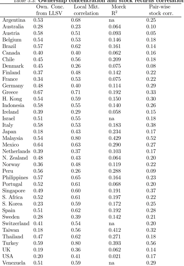
Our first measure of a country’s diversification opportunities was Local market corre-lation, a weighted average of correlations of industry stock indexes. We estimated

cor-relations between industry stock indexes in 38 countries (see Table 5.3) using monthly returns for the period 1998-2000 from Datastream stock prices.4 _{The 10 industries in} the Datastream database are: Resources, Basic Industries, General Industrials, Cyclical Consumption Goods, Non-Cyclical Consumption Goods, Cyclical Services, Non-Cyclical Services, Utilities, Information Technology, Financial. We calculated the pair-wise cor-relations among the 10 industry returns and determined the average pair-wise industry correlation with the market capitalization of each industry index as weights.

For robustness we introduced two additional measures of a country’s diversification opportunities. The first was the Pair-wise stock correlation, i.e. the average pair-wise correlation of monthly returns on single stocks for each country with the market cap-italization of each stock as weights. This is the direct empirical counterpart of the correlation coefficient in the theoretical model but it is largely affected by the number of stocks in the capital market. Our last measure of stock price synchronicity was Morck’s et al. (2000) R2_{based on the CAPM/market factor linear regression. This is the average} R2 _{(henceforth the Morck R}2_{) offirm-level regressions of bi-weekly stock returns in each} country in 1995 (see Table 5.3).

[INSERT Table (5.3) about here]

Our measure of ownership concentration was the percentage of the shares owned by the top three shareholders in the ten largest companies from La Porta et al. (1998), henceforth denoted as Ownership concentration from LLSV (see Table 5.3). We took the shares of the top three shareholders as a proxy for the shares of the controlling

4_{We also considered the correlation based on the five-year sample 1996-2000, for which a smaller} number of countries was available. The lower number of countries was the only reason why we preferred the three-year sample. Nevertheless the results of the regressions using the five-year sample were qualitatively similar, and we do not report them here.

shareholder, under the assumption that all the largest shareholders are potentially able to obtain control benefits.5

Our first set of explanatory variables were indicators of the quality of shareholder protection. We considered two widely used measures: Antidirectors rights, and Legal reserve required (the percentage of total share capital mandated by corporate law to prevent the dissolution of an existing firm) - both taken from La Porta et al. (1998). Recall that both indexes are proxies for (the inverse of) the profit diversion parameter

b.

Our main control variables are the logarithm of GNP per capita, given that richer countries may have different ownership patterns, and the logarithm of GDP because larger economies may have largerfirms which may have lower ownership concentration. We selected these variables after using a stepwise regression procedure that consid-ered all the statistically significant variables6 _{used in La Porta et al. (1998). It involved} adding and/or deleting variables from the regression analysis sequentially, depending on the F-value or the significance of the coefficients. One of the benefits of this procedure is its parsimonious selection of the explanatory variables, while one of its shortcomings is the breakdown of statistical inference. The latter was of concern to us; however, its only effect would have been to worsen the ability of parsimoniously extracted exogenous vari-ables to explain out of sample variations. Given that we obtained within-sample results

5_{As a secondary measure of ownership concentration we took the equally weighted average fraction} of firm stock market capitalization held by insiders according to Worldscope 2002 from Stulz (2005), henceforth denoted as Ownership concentration from Stulz.

6_{The variables used in the stepwise regression procedure were: the logarithm of GNP per capita,} the logarithm of GDP, the Gini coefficient for a country’s income as a proxy of the level of inequality in society, and several measures of the legal system such as Legal origin dummies (French, English, German, the omitted dummy being Scandinavian); the four measures of the quality of the legal system that La Porta et al. (1998) show to be statistically significant in their study, namely Antidirectors rights, Accounting standards, Mandatory dividend (describes whether there are rules that forcefirms to pay dividends) and Legal reserve required.

that were consistent with previous research and that we had a limited dataset, we believe that the benefits of using a stepwise regression procedure outweighed its limitations.

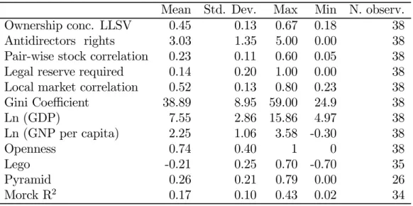
Table (5.4) displays the univariate statistics, and tables (5.5) and (5.6) the simple correlation coefficients for our variables of stock returns correlation, Ownership concen-tration, and the structural variables.

[INSERT Table (5.4) about here] [INSERT Table (5.5) about here] [INSERT Table (5.6) about here]

The univariate statistics show that Local market correlation and Ownership con-centration differ across countries. The sign of the correlation coefficients for our stock returns correlation and ownership concentration are largely as expected from our theoret-ical model. Moreover, Antidirectors rights and Local market correlation are statisttheoret-ically unrelated; indeed, despite the negative point estimate, the coefficient is not significantly different from zero. The same applies to the pair-wise stock correlation and the Morck R2 variable. The latter result is consistent with the relation found by Morck et al. (2000).7

4.2. Ownership concentration and diversification opportunities

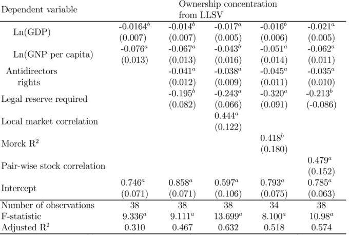
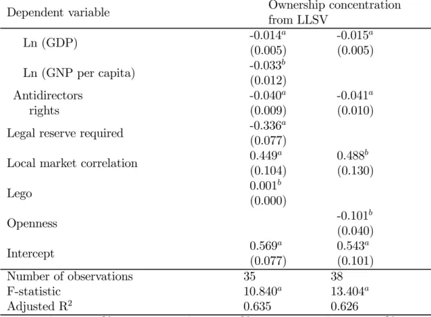
The main prediction of the model is that ownership concentration increases when di-versification opportunities decline. Table (5.7) shows the results of the regression of the LLSV ownership concentration, against measures of investor protection, and our three measures of stock market synchronicity, and structural variables.

[INSERT Table (5.7) about here]

7_{More specifically, Morck et al. (2000) find that Antidirectors rights matter for explaining stock} returns synchronicity in developed countries. We will consider this aspect later when we investigate the potential endogeneity of stock returns correlations.

The first column of Table (5.7) shows the importance of structural elements of the economy alone in explaining ownership concentration: in particular larger and richer economies have less concentrated ownership. The second column shows the importance of the quality of the legal system of investor protection in affecting ownership concen-tration. Antidirectors rights and Legal reserve required have a negative and statistically significant relationship with ownership concentration as in La Porta et al. (1998). To document the extent to which diversification opportunities affect ownership concentra-tion, in the third column we add Local market correlation to the specification in column two. An increase in Local market correlation, all else being equal, is associated with an increase in ownership concentration. In particular, Local market correlation matters in that its coefficient is significant at the 1% level, with the expected positive sign, and its impact on ownership concentration is sizeable. The estimated coefficient suggests that an increase of one standard deviation of Local market correlation (approximately +13% of Local market correlation) is associated with an increase of slightly less than half the standard deviation of ownership concentration (approximately +6% of ownership con-centration). The adjusted R2 increases substantially with respect to the regression in column two. A qualitatively similar conclusion holds if we use Morck R2 _{or Pair-wise} stock correlation for stock price synchronicity (columns four and five, respectively).8

8_{We have replicated the regressions of Table (5.7) with the Stultz measure of ownership concentration,} and the results were qualitatively similar. They are not reported here for brevity. We also considered also alternative measures of stock returns correlation, such as Equally weighted pair-wise correlation or the equally weighted correlation measure based on the same number of industries for each country. We obtained results similar to those presented in Table (5.7) and do not report them for brevity. We further considered alternative explanatory variables like stock market capitalization over GDP, average market capitalization of firms, number of listed stocks, and the results of the regressions were qualitatively unchanged. The same applied if we included the disclosure variable constructed by La Porta et al. (2005) or the Opacity measure used by Jin and Myers (2006).

4.3. The intensity of the relationship between diversification opportunities and ownership concentration

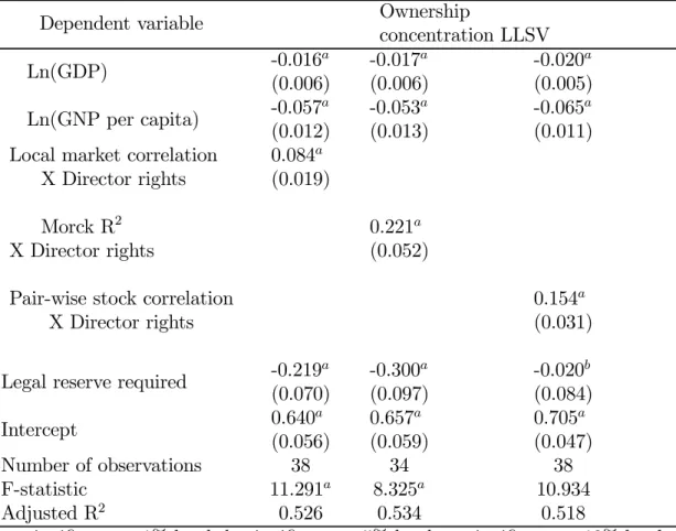
We then investigated the model’s prediction that the intensity of the relationship between the correlation of stock returns and ownership concentration is amplified by poor investor protection. In Table (5.8) a measure of investor protection is interacted with Local market correlation. For this purpose we have constructed a new variable: Directors rights, which is the negative of Antidirectors rights. The results show that the impact of Local market correlation on ownership concentration is amplified by poor investor protection. The results are robust with respect to the other two measures of stock price synchronicity used.

[INSERT Table (5.8) about here]

4.4. Pyramids and ownership concentration

The model assumed that the overall amount of diverterd profits grows with the ownership stake. In many countries, however, it is possible to obtain large control benefits even with small ownership stakes, for example through pyramids and shares with multiple votes. In cases where these alternative ways to divert profits are allowed, the impact of the stock return correlation on ownership concentration should be smaller. To test this conjecture we used the variable Pyramid, which is the percentage of not widely-held

firms controlled through pyramids at the 20% control level, obtained from La Porta et al. (1999).

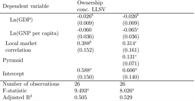
We then regressed ownership concentration against Pyramid, and the set of explana-tory and other variables used above. The results reported in Table (5.9) show that the coefficient of Pyramid is positive and significant as predicted, thus indicating that ownership is more concentrated in countries where there are more pyramidal groups.

Furthermore, the coefficient of Local market correlation has less explanatory power when the variable Pyramid is included; hence the relationship between Local market correlation and ownership concentration is weaker in countries with more pyramids.9

[INSERT Table (5.9) about here]

4.5. Diversification in an open economy

When conducting the benchmark test of the relationship between ownership concen-tration and diversification opportunities we have implicitly assumed that individuals can only invest in their own country. In what follows we investigate wether this is a valid approximation for the problem at hand, and if and how the possibility to diversify internationally affects ownership concentration.

The removal of capital controls in both developed and emerging markets has led to unparalleledfinancial openness across the world. Multi-lateral trade rounds, regional trade arrangements, and unilateral trade reforms have given rise to increased trade open-ness. However, capital market segmentation is still substantial even in the absence of strong capitalflow restrictions (see, for example, Bekaert 1995, and Nishiotis 2004). The presence of financial market segmentation has been well documented by many authors (see Stultz 2005, and Bekaert et al. 2007 among others). Financial market segmenta-tion is largely affected by indirect barriers such as political and liquidity risks, market inefficiencies, information asymmetries, poor corporate governance, different risk ap-petite, and business cycles. These barriers may affect segmentation by limiting both the ability to attract portfolio investments from foreigners and the investment abroad of local investors, the well-known home bias. The documented widespread presence of

financial market segmentation supports our assumption that the degree of closure of

9_{When we used Pair-wise stock correlation or Morck R}2_{, Pyramid was again significant with positive}

the economies in our sample is such that the relevant trade-off for an entrepreneur is between control benefits and domestic stock returns correlations.

However, even if overall there is evidence offinancial market segmentation, its degree differs among countries. We thus sought to exploit the variability of financial markets segmentation in order to determine wether it matters for ownership concentration. Since investing abroad offers additional diversification opportunities, it follows that the link between ownership concentration and the domestic stock returns correlation should be established after controlling for market segmentation.

Since the degrees of market segmentation of world equity markets and country open-ness are difficult to measure, we considered several measures of market segmentation and openness of a country10. We used the new measure of market segmentation proposed by Bekaert et al. (2007) based on the deviation of local and global price-earnings ratios (Lego). For trade openness (Openness) we used the fraction of years during the period 1965-1990 in which the country was rated as an open economy according to the crite-ria in Sachs and Warner (1995).11 _{We then regressed ownership concentration against} measures of market segmentation, a measure of trade openness, and measures of the domestic stock returns correlation and controls for structural variables.

[INSERT Table (5.10) about here]

As column 1 of table (5.10) shows, Lego is statistically significant with a positive sign. This indicates that when local market price-earnings ratios are larger than global market price-earnings ratios, ownership concentration is greater. However, measures of the domestic stock returns correlation still have a positive and significant sign. We also considered other measures used in the literature, such as the absolute value of

10_{Stulz (2005) discusses the many indexes that attempt to quantify the barriers to trade infinancial} assets and the limitations of these indices.

the deviation of local and global price-earnings ratios, Capital account openness12_{, and} Foreign Direct Investment/GDP, but these are not statistically significant. Instead, what continues to explain ownership concentration are measures of the domestic stock returns correlation, which have a positive and significant sign. Finally, trade openness (column 2) has a negative and significant impact on ownership concentration, but the domestic stock returns correlation remains significant with a positive sign. Overall, these results seem to support the view that the diversification opportunities relevant for the problem at hand are mainly domestic and that measures of financial openness do not strongly affect ownership concentration.

4.6. Endogeneity of stock returns correlations

A potential criticism is that the negative relationship identified between ownership con-centration and diversification opportunities may be spurious because diversification op-portunities may be affected by institutions. It can be argued that control benefits and public risk-return profiles both depend on the strength of institutions. Indeed Dyck and Zingales (2004) and La Porta, Lopez-de-Silanes, and Shleifer (2006) argue that private benefits of control are caused by weak institutions. Morck et al. (2000), Wurgler (2000), and Jin and Myers (2006) argue that stock price comovements are associated with weak institutions and GDP variables. If this were the case our estimation of the coefficient of the diversification opportunities variables would be biased.

Our first step toward the correct estimation of the impact of diversification opportu-nities on ownership correlation was to obtain the component of cross country variation in diversification opportunities explained by the quality of institutions and variables

12_{Quinn’s (1997) capital account openness measure is created from the volume published by the} IMF, Exchange Arrangements and Exchange Restrictions. It is scored 0-4, in half integer units, with 4 representing a fully open economy.

related to GDP. Second, we determined whether the component of diversification oppor-tunities explained by the quality of institutions and GDP variables affected cross-country differences in ownership concentration. Third, we determined whether the quality of in-stitutions and GDP variables affected ownership concentration also directly, i.e. beyond their ability to affect diversification opportunities and poor investor protection.

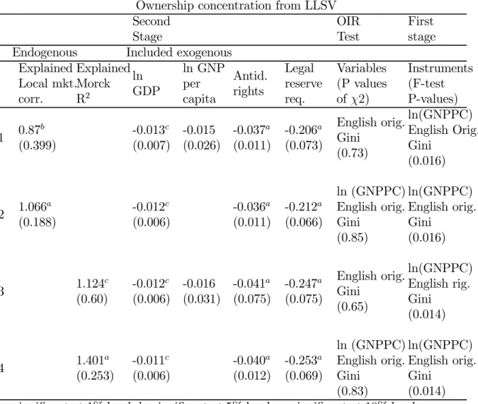
To this end we performed two-stage least squares regressions. In the first stage the dependent variable was the stock returns correlation (i.e. Local market correlation, and Morck R2) and the explanatory variables were English legal origin, which we consider to be a good exogenous instrument for the quality of institutions (as in La Porta, Lopez-de-Silanes, and Shleifer 2006). Moreover, we used the logarithm of GNP per capita, and the Gini coefficient, as a country’s gross production variables.13 In the first-stage regression we determined the component of diversification opportunities explained by the quality of institutions and GDP variables that we refer to as Explained diversification.

We then performed a second-stage regression where the dependent variable was own-ership concentration and the explanatory variables were Explained diversification, and the variables already included in previous regressions presented in Tables (5.7), i.e. the logarithm of GDP, the logarithm of GNP per capita, Antidirectors rights, Legal reserve required.

To determine whether the estimated coefficient of the Explained diversification vari-able was not biased we needed to perform an Overidentifying Restriction (OIR) test to verify wether the variables that we included in the first stage but not in the second did not affect ownership concentration directly. Specifically, the OIR tested the null hypothesis that these variables do not explain cross country ownership concentration

beyond their ability to affect it through the explanatory variables included in the second

13_{We do not show the results including also GDP because, as in Morck at al. (2000), we found that} diversification opportunities are not affected by differences in country size.

stage (i.e. Explained diversification variable, the logarithm of GDP, the logarithm of GNP per capita, Antidirectors rights, Legal reserve required, and Expropriation risk). The OIR test yields a Lagrange multiplier test statistic that under the null hypothesis is distributed as a Chi-square (m), wherem is the number of overidentifying restrictions (Davidson and MacKinnon 1993). The number of overidentifying restrictions equals the number of excluded explanatory variables in the second stage but included in the first stage minus the number of endogenous variables included as regressors in the second-stage.

Table (5.11) presents thefirst-stage least squares regressions with the F-test’s P-value and the two-stage least squares results on the LLSV ownership concentration measure with the OIR test. The null hypothesis of thefirst-stage F-test was that the explanatory variables do not capture any cross-country variation in diversification opportunities. In both the first-stage regressions with Local market correlation and Morck R2 _as depen-dent variables we reject the null hypothesis at the 2% level, thus indicating that the explanatory variables are valid. In the second stage we examined wether the component of diversification opportunities explained by our variables (i.e. the Explained diversifi ca-tion variable) explained cross-country differences in ownership concentration. We show that, the Explained diversification variable indeed enters significantly at the 1% level in both parsimonious regressions 2 and 4. The results are robust to controlling for the log-arithm of GDP, the loglog-arithm of GNP per capita, Antidirectors rights, and Legal reserve required (the other variables significant in our regressions reported in Table (5.7) and in previous research by La Porta et al. 1998); see regressions 1 and 3.14 _{The OIR test}

14_{The results were the same if we included the logarithm of GDP as explanatory variable in thefirst} stage.

did not reject the null hypothesis that the Gini index, the logarithm of GNP per capita, and the English origin variables can be excluded from the second-stage regression.15

This analysis confirms that both control benefits and public risk-return profiles are affected by the strength of institutions and country gross production variables. Neverthe-less, it also suggests that one of the channels through which the strength of institutions affects ownership concentration is diversification opportunities.16 _{These results should} mitigate concerns about the endogeneity of a country’s diversification opportunities and increase the robustness of our result that diversification opportunities matter for own-ership concentration.

[Insert Table (5.11) about here]

4.7. Reverse causality

Ownership concentration might affect the stock returns correlations, which therefore might be endogenous. To cope with the potential problem of reverse causality we needed to identify an instrument that affects stock returns correlations but not ownership con-centration. Our theoretical model suggests that this instrument could be the variance of the stock index returns. Note that variance affects correlation by construction, but not ownership structure, as shown in equations (3.11)-(3.13). To this end we performed a Hausman (1978) test.

The result of the Hausman test (not reported here for brevity but available from the authors upon request) rejected the hypothesis that Local market correlation is en-dogenous. Therefore, the Hausman test failed to reject the hypothesis that the OLS

15_{The OIR has one degree of freedom when the logarithm of GNP per capita is included in the second} stage and excluded in the OIR test because there is one endogenous variable included as regressor in the second stage (Explained diversification) and there are two excluded exogenous variables (English Origin and Gini Index). When the logarithm of GNP per capita is excluded in the second stage and included in the OIR test, there are two degrees of freedom.

16_{We repeated the above procedure using the Stultz measure of ownership concentration. Since the} results were qualitatively similar we do not report them here for brevity.

estimations shown in Table (5.7) yielded unbiased and consistent results. Nevertheless, this evidence is tentative because we used only one instrumental variable and the dataset is limited.

5. Extensions and Conclusions

This paper has developed a framework to analyze the interactions between diversifi ca-tion opportunities and ownership concentraca-tion in an environment with control benefits arising from limited legal investors protection.

We have considered a mean-variance economy where the expected returns for con-trolling and non-concon-trolling shareholders are different because the former can divert part of the profits. This offers a convenient simplified framework in which to study the gen-eral theme of the tension between the need to diversify the portfolio of the controlling shareholder and the small amount of external finance that can be raised when there is ample opportunity to expropriate outsiders.

We have obtained a number of results. First,when stock returns correlations increase, each controlling shareholder invests a larger share of his wealth in the asset that he con-trols and a lower share in the assets that he does not control. Second, as a consequence, ownership becomes more concentrated when diversification opportunities decline. This is because an increase in correlation lowers both (i) the loss of forgone diversification opportunities from concentrated portfolios and (ii) the overall level of control benefits that non-controlling investors are willing to tolerate to achieve the excess returns on the risky investments.

Our objective in attempting to integrate analysis of firms’ governance and owner-ship structure into a general equilibrium economy with different levels of stock returns correlation has been to show that correlation is an important variable in explanation

of ownership structure. This theoretical result has been confirmed by the empirical analysis. Ownership is more concentrated in countries where stock returns correlations are higher. This effect is weaker in countries where investors are able to retain control without sacrificing portfolio diversification, e.g. through pyramids, and the intensity of the relationship between the stock returns correlation and ownership concentration is amplified by poor investor protection. Local market correlation is still a relevant variable for ownership concentration even after controlling for international portfolio diversifi ca-tion. We have also addressed the concern that the impact of stock returns correlations on ownership concentration might be spurious because both are affected by institutions. We have shown that the stock returns correlation is one of the channels through which institutions affect ownership concentration.

The foregoing analysis can be extended in several directions, theoretical, institu-tional and empirical. At the theoretical level, the model can be extended to investigate an economy where entrepreneurs compete on profit diversion in order to attract outside funds. The more general issue of harmonization versus competition in corporate gover-nance law across countries can be tackled using our framework. At the empirical level, our analysis can also be conducted for a cross section of firms within the same country. However, deeper understanding of the problems at hand requires better measures of profit diversion, and control benefits.

Appendix

Proof of Proposition 3.1

First to be proved is that there is a sufficiently high level of ρ < 1 such that when

b >0and the diversification opportunities decline each entrepreneur invests more in his company. Observe from (3.4) that

∂x∗ ii ∂ρ =− (m₋b₋1) (ρ2_{+ 1)} −2ρ(m₋1) λσ2_{(−1 +ρ}2₎2 . (5.1) Thus ∂x∗ii ∂ρ |ρ=0= 0, and limρ→1 ∂x∗ ii

∂ρ > 0. Thus by continuity there exists a ρ, such that

0 < ρ < 1, above which the result holds. Second, from (3.5) it is easy to see that ∂x∗

ji

∂ρ <0. ¥

Proof of Proposition 3.2

From (3.11) the derivative of αii w.r.t. ρ is

∂α∗ii

∂ρ =

b

(₋1 +ρ)2((m₋1₋b) (W3+ 2) +b)

>0. (5.2) From (3.12) the derivative of α∗

ji w.r.t. ρ is ∂α∗ji ∂ρ =− b (₋1 +ρ)2((m₋1₋b) (W3+ 2)) <0. (5.3) Similarly for (3.13).Taking the derivatives of (5.2), and (5.3) w.r.t. bwe obtain, respec-tively ∂³∂α∗ii ∂ρ ´ ∂b = (W3+ 2) (m−1) (ρ₋1)2[W3(1−m) + 2 (1−m) +b(W3+ 1)]2 >0, (5.4) and ∂³∂α∗ji ∂ρ ´ ∂b =− (m₋1) (W + 2) (2m₋2₋b+W m₋W ₋W b)2(₋1 +ρ)2 <0. (5.5) ¥

The model with n+ 1 assets and n+ 1 individuals

Letx0

j = (xj1, ..., xjn) be the row vector of the proportion of the wealth of individual

j, j = 1, ..., n+ 1, invested in assets 1, ..., n. Using the accounting identity linking the individual portfolio shares and the total investment in the risky assets

Ii =x1iW1+, ...,+xn+1iWn+1, i= 1, ..., n, (5.6) the portfolio problem becomes:

for each entrepreneur

max xj Vj = ∙ 1 +x0_jy₋ λσ 2 2 x 0 jΩxj ¸ Wj +b n+1 X k=1 Wkx0kej, j = 1, . . . , n (5.7) and for the household

max xn+1 Vn+1 = ∙ 1 +x0_n+1y₋ λσ 2 2 x 0 n+1Ωxn+1 ¸ Wn+1 (5.8)

where y0 _{= ((m−1−b), ...,(m−1−b)) denotes the row vector of the expected rates} of return on the risky assets,ej represents thej−th column vector of the canonical base in_<n_,17 _{andΩis the n}

×nmatrix of the correlation coefficients between the returns on the risky assets.18

The terms in the square brackets of (5.7) and (5.8) represent the risk-adjusted rate of portfolio return per unit of wealth, and the last term of (5.7) represents the profit diverted by entrepreneurj as a result of the investment decisions of all the individuals. If the conditions for the invertibility of the matrixΩ are satisfied, i.e. if

|Ω_{| 6}= 0 which implies ρ₆= 1, ρ₆=₋ 1

n₋1, (5.9)

17_{That is the transpose ofej,ise}0

j = (0, ...,1, ...,0). 18_FormallyΩ= ⎛ ⎜ ⎜ ⎝ 1 ρ ... ρ ρ 1 ... ... ... ... ... ρ ρ ... ρ 1 ⎞ ⎟ ⎟ ⎠.

then Ω−1 = ⎛ ⎜ ⎜ ⎜ ⎜ ⎜ ⎜ ⎝ (n−2)ρ+1 A ... − ρ A . . . −Aρ ... (n−2)ρ+1 A ⎞ ⎟ ⎟ ⎟ ⎟ ⎟ ⎟ ⎠ (5.10) with A≡(1−ρ) (1 + (n−1)ρ).

The first order conditions of the optimization of (5.7) and (5.8) s.t. (5.6) and the resource constraint In+1 =W −Pn_i=1Ii are

y₋λσ2xjΩ+bej = 0, j= 1, . . . , n; y−λσ2xn+1Ω= 0. (5.11) The vector of the optimal shares of risky assets in the portfolios of then+ 1 individuals are

for the entrepreneurs x∗_j = 1

λσ2Ω

−1_(y+be

j), j = 1, . . . , n (5.12) for the household x∗_n+1= 1

λσ2Ω

−1_{y. (5.13)}

Solving for x∗_j and x∗_n+1 we obtain the optimal portfolio shares

x∗_ii= m−1 λσ2 ∙ (1₋ρ) A ¸ + (n−1)ρb λσ2_A (5.14) x∗_ji = m−1 λσ2 ∙ (1₋ρ) A ¸ − b λσ2_A (5.15) i, j = 1, ..., nwith i₆=j x∗_n+1i = m−1 λσ2 ∙ (1₋ρ) A ¸ −b(1_λσ−2_Aρ). (5.16) Using equations (5.6), (5.14)-(5.16) we obtain the level of investment in the risky assets

I_i∗ = x∗_ii+x_ji∗(n₋1) +x∗_n+1iWn+1 (5.17) = m−1 λσ2 ∙ (1₋ρ) A ¸ + (n−1)ρb λσ2_A + (n−1) ∙ m₋1 λσ2 (1₋ρ) A − ρb λσ2_A ¸ = m−1 λσ2 (1₋ρ) A (1 +n−1 +Wn+1)− (n₋1) (1₋ρ)b λσ2_A +Wn+1 (1₋ρ)b λσ2_A .

Using the accounting identities α∗_ji = Wn+1 I∗ i x∗_j,i, j = 1, ...n, i= 1, ...n (5.18) α∗n+1,i= Wn+1 I∗ i x∗n+1,i (5.19) we obtain the ownership structure. For example entrepreneur i owns α∗ii of the asset that he controls with

α∗ii=

(m₋1) (1₋ρ) + (n₋1)ρb

(m₋1) (1₋ρ) (n+Wn+1) + (n−1)ρb−(n−1)b−Wn+1b(1−ρ)

. (5.20)

From (5.20) taking derivatives, and recalling that m₋1₋ b > 0 by assumption, we obtain ∂α∗ ii ∂ρ = (n₋1)b (₋1 +ρ)2((m₋1₋b) (Wn+1+n) +b) >0. (5.21) Taking the derivative of (5.21) w.r.t. bwe obtain

∂ ³_∂α∗ ii ∂ρ ´ ∂b = (n₋1) (m₋1) (Wn+1+n) (ρ₋1)2[₋(m₋1₋b) (Wn+1+n)−b] 2 >0. (5.22)

References

[1] Bekaert, G. (1995) "Market integration and investment barriers in emerging equity markets"World Bank Economic Review 9, 75-107.

[2] Bekaert, G., C, Harvey, C. Lundblad, and S. Siegel (2007) "What Segments Equity Markets?" Working Paper Duke University.

[3] Bennedsen, M., and D. Wolfenzon (2000) “The Balance of Power in Closely Held Corporations” Journal of Financial Economics, 58, 113-139.

[4] Burkart M., D. Gromb, and F. Panunzi (1998) “Why Higher Takeover Premia Protect Minority Shareholders”Journal of Political Economy 106, 172-204.

[5] Castro R., G. L. Clementi, and G. MacDonald (2004) “Investor Protection, Optimal Incentives, and Economic Growth”Quarterly Journal of Economics August, 1131-1175.

[6] Demsetz, H. and K. Lehn (1985) “The Structure of Corporate Ownership: Causes and Consequences” Journal of Political Economy 93, 1155-77.

[7] Davidson, R. and J.G. MacKinnon (1993)Estimation and inference in econometrics

Oxford University Press, Oxford, UK.

[8] Dyck, A. and L. Zingales (2004) “Private Benefits of Control: An International Comparison”Journal of Finance 59, 537-600.

[9] Hausman, J. (1978) “Specification tests in econometrics” Econometrica 46, 1251-1271.

[10] Jin, L. and S. Myers (2006) “R-Squared around the world: new theory and new tests” Journal of Financial Economics 79, 257-292.

[11] Kumar, K., R. Rajan, and L. Zingales (1999) “What Determines Firm Size?’, NBER Working Paper 7208.

[12] La Porta, R., F. Lopez-de-Silanes, and A. Shleifer (1999) “Corporate ownership around the world” Journal of Finance 54, 471-517.

[13] La Porta, R., F. Lopez-de-Silanes, and A. Shleifer (2000) “Investor Protection and Corporate Valuation” Journal of Financial Economics 59, 3-27.

[14] La Porta, R., F. Lopez-de-Silanes, and A. Shleifer (2006) “What Works in Securities Laws” Journal of Finance LXI, 1-32.

[15] La Porta, R., F. Lopez-de-Silanes, A. Shleifer, and R. Vishny (1997) “Legal Deter-minants of External Finance” Journal of Finance 52, 1131-1130.

[16] La Porta, R., F. Lopez-de-Silanes, A. Shleifer, and R. Vishny (1998) “Law and Finance”Journal of Political Economy 106, 1113-1155.

[17] Levine, R. and S. Zervos (1998) “Stock Markets, Banks, and Economic Growth”

[18] Morck, R., B. Yeung, and W. Yu (2000) “The Information Content of Stock Mar-kets: Why do Emerging Markets have Synchronous Stock Price Movements?” Jour-nal of Financial Economics 58, 215-260.

[19] Nenova, T. (2003) “The Value of Corporate Voting Rights and Control: A Cross-Country Analysis”Journal of Financial Economics 68, 325-351.

[20] Nishiotis, G. (2004) "Do Indirect Investment Barriers Contribute to Capital Market Segmentation?" Journal of Financial and Quantitative Analysis 39, 613-630. [21] Pagano, M., and A. Röell (1998) “The Choice of Stock Ownership Structure:

Agency Costs, Monitoring, and the Decision to Go Public” Quarterly Journal of Economics, 113, 187-226.

[22] Quinn, D. (1997) The correlates of changes in international financial regulation,

American Political Science Review 91, 531-551.

[23] Sachs, J., and A. Warner (1995) “Economic Reform and the Progress of Global Integration” Brookings Paper on Economic Activity 1, 1-118.

[24] Shleifer, A., and D. Wolfenzon (2002) “Investor Protection and Equity Markets”

Journal of Financial Economics 66, 3-27.

[25] Stulz, R. M. (2005) “The Limits of Financial Globalization”Journal of Finance 60, 1595-1638.

[26] Wurgler, J. (2000) “Financial Markets and the Allocation of Capital” Journal of Financial Economics 58, 187-214.

[27] Zingales, L. (1994) “The Value of the Voting Right: a Study of the Milan Stock Exchange Experience” Review of Financial Studies 7, 125-148.

[28] Zingales, L. (1995) “Inside ownership and the decision to go public” Review of Economic Studies 62, 425-448.

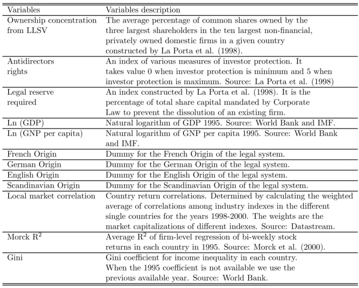
Table 5.1: Variables description

Variables Variables description

Ownership concentration The average percentage of common shares owned by the

from LLSV three largest shareholders in the ten largest non-financial,

privately owned domesticfirms in a given country

constructed by La Porta et al. (1998).

Antidirectors An index of various measures of investor protection. It

rights takes value 0 when investor protection is minimum and 5 when

investor protection is maximum. Source: La Porta et al. (1998)

Legal reserve An index constructed by La Porta et al. (1998). It is the

required percentage of total share capital mandated by Corporate

Law to prevent the dissolution of an existingfirm.

Ln (GDP) Natural logarithm of GDP 1995. Source: World Bank and IMF.

Ln (GNP per capita) Natural logarithm of GNP per capita 1995. Source: World Bank

and IMF.

French Origin Dummy for the French Origin of the legal system.

German Origin Dummy for the German Origin of the legal system.

English Origin Dummy for the English Origin of the legal system.

Scandinavian Origin Dummy for the Scandinavian Origin of the legal system.

Local market correlation Country return correlations. Determined by calculating the weighted

average of correlations among industry indexes in the different

single countries for the years 1998-2000. The weights are the

market capitalizations of different indexes. Source: Datastream.

Morck R2 Average R2 of firm-level regression of bi-weekly stock

returns in each country in 1995. Source: Morck et al. (2000).

Gini Gini coefficient for income inequality in each country.

When the 1995 coefficient is not available we use the

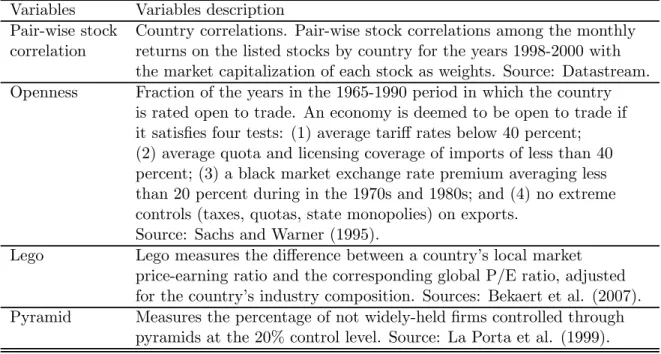
Table 5.2: Variables description continued

Variables Variables description

Pair-wise stock Country correlations. Pair-wise stock correlations among the monthly

correlation returns on the listed stocks by country for the years 1998-2000 with

the market capitalization of each stock as weights. Source: Datastream.

Openness Fraction of the years in the 1965-1990 period in which the country

is rated open to trade. An economy is deemed to be open to trade if it satisfies four tests: (1) average tariffrates below 40 percent; (2) average quota and licensing coverage of imports of less than 40 percent; (3) a black market exchange rate premium averaging less than 20 percent during in the 1970s and 1980s; and (4) no extreme controls (taxes, quotas, state monopolies) on exports.

Source: Sachs and Warner (1995).

Lego Lego measures the difference between a country’s local market

price-earning ratio and the corresponding global P/E ratio, adjusted for the country’s industry composition. Sources: Bekaert et al. (2007).

Pyramid Measures the percentage of not widely-heldfirms controlled through

Table 5.3: Ownership concentration and stock returns correlations. Own. Conc. from LLSV Local Mkt. correlation Morck R2 Pair-wise stock corr. Argentina 0.53 0.68 na 0.25 Australia 0.28 0.23 0.064 0.10 Austria 0.58 0.51 0.093 0.05 Belgium 0.54 0.53 0.146 0.18 Brazil 0.57 0.62 0.161 0.14 Canada 0.40 0.40 0.062 0.16 Chile 0.45 0.56 0.209 0.18 Denmark 0.45 0.26 0.075 0.08 Finland 0.37 0.48 0.142 0.22 France 0.34 0.53 0.075 0.22 Germany 0.48 0.40 0.114 0.29 Greece 0.67 0.71 0.192 0.33 H. Kong 0.54 0.59 0.150 0.30 Indonesia 0.58 0.55 0.140 0.26 Ireland 0.39 0.29 0.058 0.15 Israel 0.51 0.55 na 0.18 Italy 0.58 0.53 0.183 0.38 Japan 0.18 0.43 0.234 0.17 Malaysia 0.54 0.80 0.429 0.52 Mexico 0.64 0.63 0.290 0.27 Netherlands 0.39 0.37 0.103 0.17 N. Zealand 0.48 0.43 0.064 0.20 Norway 0.36 0.48 0.119 0.22 Peru 0.56 0.26 0.288 0.09 Philippines 0.57 0.65 0.164 0.23 Portugal 0.52 0.61 0.068 0.20 Singapore 0.49 0.60 0.191 0.37 S. Africa 0.52 0.61 0.197 0.22 S. Korea 0.23 0.59 0.172 0.25 Spain 0.51 0.62 0.192 0.28 Sweden 0.28 0.39 0.142 0.21 Switzerland 0.41 0.54 na 0.20 Taiwan 0.18 0.56 0.412 0.32 Thailand 0.47 0.62 0.271 0.18 Turkey 0.59 0.80 0.393 0.56 UK 0.19 0.36 0.062 0.14 USA 0.20 0.41 0.021 0.17 Venezuela 0.51 0.59 na 0.29

Table 5.4: Univariate statistics of the variables

Mean Std. Dev. Max Min N. observ. Ownership conc. LLSV 0.45 0.13 0.67 0.18 38 Antidirectors rights 3.03 1.35 5.00 0.00 38 Pair-wise stock correlation 0.23 0.11 0.60 0.05 38 Legal reserve required 0.14 0.20 1.00 0.00 38 Local market correlation 0.52 0.13 0.80 0.23 38 Gini Coefficient 38.89 8.95 59.00 24.9 38

Ln (GDP) 7.55 2.86 15.86 4.97 38 Ln (GNP per capita) 2.25 1.06 3.58 -0.30 38 Openness 0.74 0.40 1 0 38 Lego -0.21 0.25 0.70 -0.70 35 Pyramid 0.26 0.21 0.79 0.00 26 Morck R2 0.17 0.10 0.43 0.02 34

Table 5.5: Correlation between main variables

1 2 3 4 5 6 7 8 1 Ownership conc. LLSV 1 -0.37 a _0.29b _-0.25c _0.50a _{-0.15 -0.49}a _0.23c 2 Antidirectors rights 1 -0.14 -0.28 b _{-0.13 -0.02 0.09 -0.17} 3 Pair-wise Stock correlation 1 0.14 0.70 a _0.46a _-0.23c _0.64a 4 Legal reserves required 1 0.14 0.11 0.09 0.46 a 5 Local market correlation 1 0.14 b _-0.45a _0.59a 6 Ln (GDP) 1 -0.33b 0.43a 7 Ln (GNP per capita) 1 -0.49a 8 Morck R2 ₁ N. Observations 38 38 38 38 38 38 38 34

Table 5.6: Correlation between main variables (continued)

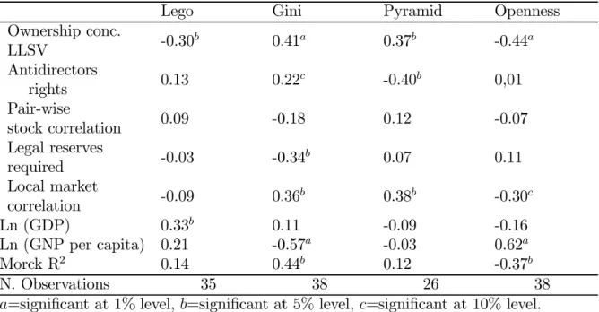
Lego Gini Pyramid Openness

Ownership conc. LLSV -0.30 b _0.41a _0.37b _-0.44a Antidirectors rights 0.13 0.22 c _-0.40b _0,01 Pair-wise stock correlation 0.09 -0.18 0.12 -0.07 Legal reserves required -0.03 -0.34 b _{0.07 0.11} Local market correlation -0.09 0.36 b _0.38b _-0.30c Ln (GDP) 0.33b _{0.11 -0.09 -0.16} Ln (GNP per capita) 0.21 -0.57a -0.03 0.62a Morck R2 _{0.14 0.44}b _{0.12 -0.37}b N. Observations 35 38 26 38

Table 5.7: Regression of LLSV ownership concentration on local market

cor-relation, Morck R2_{,pair-wise stock correlation, investor protection and}

econ-omy structural variables (Robust standard errors in parentheses).

Dependent variable Ownership concentration from LLSV Ln(GDP) -0.0164 b (0.007) -0.014b (0.007) -0.017a (0.005) -0.016b (0.006) -0.021a (0.005) Ln(GNP per capita) -0.076 a (0.013) -0.067a (0.013) -0.043b (0.016) -0.051a (0.014) -0.062a (0.011) Antidirectors rights -0.041a (0.012) -0.038a (0.009) -0.045a (0.011) -0.035a (0.010) Legal reserve required -0.195

b (0.082) -0.243a (0.066) -0.320a (0.091) -0.213b (-0.086) Local market correlation 0.444

a (0.122)

Morck R2 0.418b

(0.180)

Pair-wise stock correlation 0.479

a (0.152) Intercept 0.746 a (0.071) 0.858a (0.071) 0.597a (0.106) 0.793a (0.075) 0.785a (0.063) Number of observations 38 38 38 34 38 F-statistic 9.336a _9.111a _13.699a _8.100a _10.98a Adjusted R2 0.310 0.467 0.632 0.518 0.574

Table 5.8: Regression of ownership concentration on the product among local market correlation and investor protection and economy structural variables (Robust standard errors in parentheses).

Dependent variable Ownership

concentration LLSV Ln(GDP) -0.016 a (0.006) -0.017a (0.006) -0.020a (0.005) Ln(GNP per capita) -0.057 a (0.012) -0.053a (0.013) -0.065a (0.011) Local market correlation

X Director rights 0.084a (0.019) Morck R2 X Director rights 0.221a (0.052) Pair-wise stock correlation

X Director rights

0.154a (0.031) Legal reserve required -0.219

a (0.070) -0.300a (0.097) -0.020b (0.084) Intercept 0.640 a (0.056) 0.657a (0.059) 0.705a (0.047) Number of observations 38 34 38 F-statistic 11.291a _8.325a _10.934 Adjusted R2 _{0.526 0.534 0.518}

Table 5.9: Regression of ownership concentration on local market correlation, pair-wise stock correlation, pyramid, and structural variables (Robust stan-dard errors in parentheses).

Dependent variable Ownership conc. LLSV Ln(GDP) -0.026 b (0.009) -0.026b (0.009) Ln(GNP per capita) -0.060 (0.036) -0.065c (0.036) Local market correlation 0.388b (0.152) 0.314c (0.161) Pyramid 0.131 c (0.071) Intercept 0.588 a (0.150) 0.606a (0.140) Number of observations 26 26 F-statistic 9.493a _8.026a Adjusted R2 _{0.505 0.529}