Lasso model selection in multi-dimensional contingency tables?

contingency tables?

Gilbert MacKenzie

and Susana Conde

ENSAI, France and University of Limerick, Ireland

2 _{Manchester University, UK. and The University of Glasgow, UK.}

Email: [email protected] and [email protected]

Abstract: We develop a Smooth Lasso for sparse, high dimensional, contingency tables and compare its performance with the usual Lasso and with the now classical backwards elimination algorithm. In simulation, the usual Lasso had great difficulty identifying the correct model. Irrespective of the sample size, it did not succeed in identifying the correct model in the simulation study! By comparison the smooth Lasso performed better improving with increasing sample size. The backwards elimination algorithm also performed well and was better than the Smooth Lasso at small sample sizes. Another potential difficulty is that Lasso methods do not respect the marginal constraints on hierarchy and so lead to non-hierarchical models which are unscientific. Furthermore, even when one can demonstrate, classically, that some effects in the model are inestimable, the Lasso methods provide penalized estimates. These problems call Lasso methods into question.

Keywords: False estimation, Lasso, Model selection, Non-hierarchical models, Smooth Lasso

1

Introduction

Sparse contingency tables arise often in genetic, bioinformatic and database applications. Then the target is to estimate the dependence structure be-tween the variables modelled via the interaction terms in a log-linear model. High dimensionality will force attention on identifying important low-order interactions - a technical advance since most model selection work relies only on main effects.

Penalized likelihood attaches a penalty function of the parameters to the likelihood in order to achieve some purpose such as smoothing (Eilers and Marx, 1996), or sparsity (Freidman, 2008). Using the LASSO (L1-norm

penalty), some of the parameters go to zero allowing a more parsimonious model to be found. Dahinden (2007) extended the LASSO (Tibrishani, 1996) to contingency tables and log-linear models. However, in the Lasso the penalty is a non-differentiable function of the parameters thus necessi-tating specialized optimization algorithms.

We present the smooth LASSO, a penalized likelihood, which does not require specialized optimization algorithms such as the method of coordi-nate descent. It uses a convex, parametric, analytic penalty function that asymptotically approximates the LASSO: minimization is accomplished us-ing standard Newton-Raphson algorithms and standard errors are avail-able.

2

Model Formulation

2.1 Log-linear modelling

Assume X1, . . . , Xv correlated binary variables (off=0, on=1) and these form a v-dimensional contingency table with q = 2v _{cells. Let Y}

i be the random variable indicating the frequency in theith cell,i= 1, . . . , q and let µi = E(Yi). We consider a log-linear regression model: log(µ) = ATθ whereA is a (q×p) design matrix of fixed constants with typical element

aij, and θ is a vector with p dimensions measuring the influence of the effects (constant, main effects and interactions) on the response vector of countsY. We use Yates’ design matrix coding scheme whence the columns of A are orthogonal. Finally, let n = Pq

i=1Yi denote the total number of observations. Estimation is via the log-likelihood, which may be taken in Poisson form: `(θ|y) ∝ Pq

i=1{yi(aTiθ)−exp(aTi θ)}, as the maximum likelihood estimators are the same in multinomial and independent Poisson schemes provided Pq

i=1µi = n (Birch 1963). The log-likelihood may be

maximized numerically using iterative proportional fitting or by generating the design matrixAand using thenlmprocedure in the R software package.

2.2 A Smooth LASSO

The penalized log-likelihood is:

`λ(θ) =`(θ)−penλ (1) where pen_λ, is the penalty term,λ >0. For the LASSO pen_λ=λPp

j=2|θj| omitting the intercept term and for the Smooth LASSO pen_λ=λPp

j=2Qω(θj)

where Qω(θj) = ωloghcoshθj_ωifor a constantω that regulates the ap-proximation of the function to that of the absolute value function (Salje et al, 2005). Note that Qω(θj)∈ C∞, the set of functions that are infinitely differentiable, and is convex. Following we define the maximum penalised likelihood estimator (MPLE) as

ˆ

θ:= arg max

θ∈Θ{`(θ)−penλ(θ)}. (2)

We should more properly write ˆθλ, rather than ˆθ, but the dependence on

λwill be understood in what follows. For a largeλ, all the estimates go to 0 and for λ= 0, there is no constraint, whence ˆθλ=0 is equivalent to the

3

Non-hierarchical model

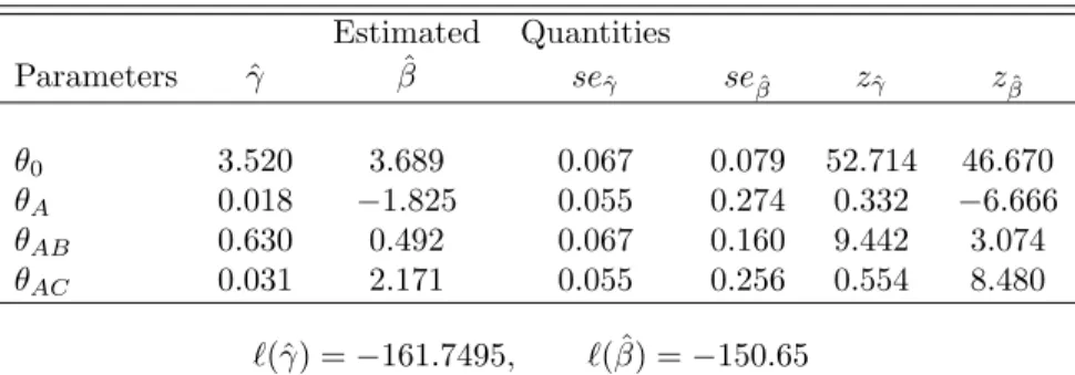
We digress to make an important methodological point by comparing Yates’ and Binary design matrix coding schemes in a non- hierarchical model using a well known example. Agresti (2002) gave the following 23 _tabley0_{= (19,} 11, 0, 6, 132, 52, 9, 97) of counts classified by: A = defendant’s race (0. white, 1. black), B = victim’s race (0. white, 1. black) and C = death penalty (0. yes, 1. no). The contingency table is written in vector notation in which the leftmost subscript varies fastest. Table 1 shows the result of

TABLE 1: Comparison of Yates’ and binary coding schemes when fitting a non-hierarchical model comprising A, AB, AC.

Estimated Quantities Parameters ˆγ βˆ seˆγ se_βˆ zˆγ z_βˆ θ0 3.520 3.689 0.067 0.079 52.714 46.670 θA 0.018 −1.825 0.055 0.274 0.332 −6.666 θAB 0.630 0.492 0.067 0.160 9.442 3.074 θAC 0.031 2.171 0.055 0.256 0.554 8.480 `(ˆγ) =−161.7495, `( ˆβ) =−150.65

fitting the non-hierarchical model A, AB, AC with with Yates’ (ˆγ) and Binary ( ˆβ) design matrices. We have the same data, the same model, but the likelihoods differ and the effects have different interpretations in the two models. This simple example shows that we should restrict model selection to hierarchical models.

Even when fitting hierarchical models, only effects in the generating set of the fitted model are invariant to the choice of design matrix. The applica-tion of Wald tests to other effects is mistaken. The likelihoods, however, are invariant. These findings apply toallstatistical models with interaction terms.

4

Lasso Model Selection

4.1 Simulation

We conducted a small simulation study designed to study the percentage of correct models identified by three algorithms: Backwards Elimination, the usual Lasso and the Smooth Lasso. For the purposes of illustration we sim-ulated a 25 contingency table when the main effects model was true. The number of replications wasm= 1000 and we started with the all 2-way in-teractions design-matrix. For the backwards elimination method we used a

TABLE 2: Simulation: Percentage of correct models identified by three methods.

Estimation Methods

Sample size BE Lasso SL-95

50 62.3 0* 0.1

100 51.6 0 11.8

500 33.0 0 50.1

1000 29.2 0 51.6

∗ _{The Lasso persistently over fits effects.}

R function written Conde (2011), for the usual Lasso we used theglmnetR package and for the Smooth Lasso we used another R function, which called

nlm. The tuning parameterλwas estimated by 10 fold cross-validation in the Lasso functions. The sample sizes studied were:n= 50,100,500,1000. For the Smooth Lasso one must pick a level of statistical significance, as with ordinary regression methods (Conde & MacKenzie, 2010). Thus SL-95 corresponds to the 5% level. It will be noticed that the 5% level produces poor results when the sample size is small, but improves with increasing sample size, while the classical Backward Elimination algorithm performs better for smaller sample sizes.

4.2 Obesity Data Analysis

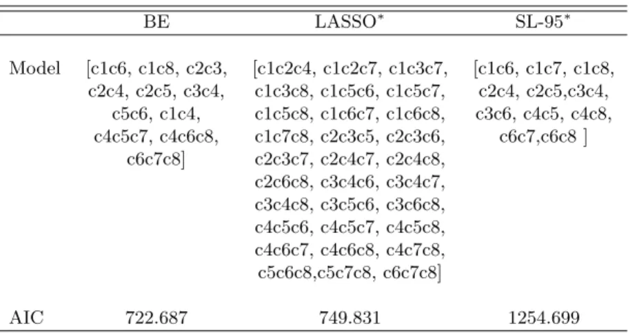
We now present the results of analysing a set of obesity data comprising 8 binary comorbidities measured onn= 5550 patients. The resulting con-tingency table has 28 cells of which 45.3% are zero cells. We compare the three algorithms described above using the same fitting methods. Table 3 presents thegenerating sets defining the final models together with their AICs. Several interesting features emerge.

First the fitted Lasso-based solution comprised non-hierarchical models. Each non-hierarchical model was then augmented by adding in effects to produce a minimum hierarchical model. The models were re-estimated (Ta-ble 3). Unfortunately, this idea does not always work - often, in sparse tables, one finds that minimum hierarchical model contains effects which are estimable, whence one is stuck with a Lasso solution which is non-hierarchical. Such solutions are unscientific.

A second problem arises with the Lasso methods investigated. If one pre-processes the table one can identify effects which are inestimable in the classical paradigm (using a theorem due to the first author). On first notic-ing this we hoped that if the Lasso was gonotic-ing to produce a sparse model it would somehow identify the inestimable effects and shrink these to zero.

TABLE 3: Generating sets of models found by Backwards Elimination, LASSO and Smooth LASSO.

BE LASSO∗ SL-95∗ Model [c1c6, c1c8, c2c3, [c1c2c4, c1c2c7, c1c3c7, [c1c6, c1c7, c1c8, c2c4, c2c5, c3c4, c1c3c8, c1c5c6, c1c5c7, c2c4, c2c5,c3c4, c5c6, c1c4, c1c5c8, c1c6c7, c1c6c8, c3c6, c4c5, c4c8, c4c5c7, c4c6c8, c1c7c8, c2c3c5, c2c3c6, c6c7,c6c8 ] c6c7c8] c2c3c7, c2c4c7, c2c4c8, c2c6c8, c3c4c6, c3c4c7, c3c4c8, c3c5c6, c3c6c8, c4c5c6, c4c5c7, c4c5c8, c4c6c7, c4c6c8, c4c7c8, c5c6c8,c5c7c8, c6c7c8] AIC 722.687 749.831 1254.699

*Minimal hierarchical model that includes the effects in the support. For the smooth LASSO,ω= 1.

However this is not the case and we have many examples of the Lasso and Smooth Lasso solutions producing penalized estimates of inestimable effects. One might be tempted to regard this as an “advantage”, but this seems n¨aive. The solution is inconsistent with the classical theory. One pos-sible explanation is that the penalized likelihoods have a Bayesian inter-pretation in which the penalty plays the role of a prior. So false estimation of inestimable effects may just correspond to a value assigned by the prior. If so, this is yet another reason for discarding such solutions.

Accepting these caveats, we note that: (a) the BE algorithm always pro-duces a hierarchical model, (b) the BE algorithm is best as judged by the AIC, (c) it is also fastest, (d) the Lasso is not the sparsest model and (e) the smooth LASSO is much more parsimonious than the LASSO. These are consistent findings in our work.

5

Discussion

There is, apparently, a highly impressive literature on Lasso methods. It is, however, predicated on model selection based on main effects models. In the presence of interactions, Lasso methods will often fail to produce scientific models. It has been argued that group Lasso methods provide one answer to this problem, but they require multiple tuning parameters, one for each class of interactionsanticipated in the final solution. Accordingly, they are prohibitively computationally expensive. Other authors have argued for weak hierarchy (Bien et al, 2013). Their arguments are not compelling

and difficult to implement. Moreover, it is well known that the Lasso lacks the oracle property and the results in Table 2 confirm this. However, the results suggest that this may not be the case for the Smooth Lasso, a finding which requires further investigation. To our knowledge the problem of false estimation has not previously been reported. All these issues raise serious questions about the usefulness of Lasso methods for model selection.

Acknowledgments: We acknowledge the help and support of Professor Victor Kiri, of FVJK consultants, UK. The second author works on the MI-MOMICS project in the Centre of Biostatistics in Manchester University, UK

References

Agresti, A. (2002). Categorical Data Analysis. John Wiley & Sons, Inc., Hobo-ken, New Jersey:Wiley-Interscience, 2nd ed.

Bien, J., Taylor, J. and Tibrishani, R. (2013). A lasso for hierarchical interac-tions. The Annals of Statistics 41, 11111141.

Birch, M. W. (1963). Maximum Likelihood in Three-Way Contingency Ta-bles. Journal of the Royal Statistical Society. Series B (Methodological) 25, 220233.

Conde, S. (2011). Interactions: Log-Linear Models in Sparse Contingency Tables. Ph.D. thesis, University of Limerick, Ireland.

Conde, S. & MacKenzie, G. (2011). LASSO Penalised Likelihood in High-Dimensional Contingency Tables. In Proceedings of the 26th International Workshop on Statistical Modelling, Valencia, D. Conesa, A. Forte, A. et al. eds.

Dahinden, C., Parmigiani, G., Emerick, M.C. and B¨uhlmann, P. (2007). Penal-ized likelihood for sparse contingency tables with an application to full-length cDNA libraries.BMC Bioinformatics,8:476.

Eilers, P.H.C. and Marx, B.D. (1996). Flexible smoothing using B-splines and penalized likelihood (with Comments and Rejoinder). Statistical Science,

11(2)89-121.

Friedman, J.H. (2008). Fast Sparse Regression and Classification. In:Proceedings of the 23rd International Workshop on Statistical Modelling, Utrecht, 27-57. Ed.: Eilers, P.H.C.

Salje, Ekhard K. H., Hayward S.A. and Lee W.T. (2005). Ferroelastic phase transitions:structure and microstructure. Acta Crystallographica Section A 61, 318.

Tibshirani, R. (1996). Regression Shrinkage and Selection via the Lasso.Journal of the Royal Statistical Society,58(1)267-288.