Statistical Methods for Panel Studies with Applications in Environmental Epidemiology

(1)

Statistical Methods for Panel Studies with Applications in

Environmental Epidemiology

(Article begins on next page)

The Harvard community has made this article openly available.

Please share

how this access benefits you. Your story matters.

Citation

No citation.

Accessed

February 19, 2015 10:55:13 AM EST

Citable Link

http://nrs.harvard.edu/urn-3:HUL.InstRepos:10121973

Terms of Use

This article was downloaded from Harvard University's DASH

repository, and is made available under the terms and conditions

applicable to Other Posted Material, as set forth at

http://nrs.harvard.edu/urn-3:HUL.InstRepos:dash.current.terms-of-use#LAA

(2)

(3)

Statistical Methods for Panel Studies with

Applications in Environmental Epidemiology

A thesis presented

by

Alfa Ibrahim Mouk´e Yansan´e

to

The Department of Biostatistics

in partial fulfillment of the requirements

for the degree of

Doctor of Philosophy

in the subject of

Biostatistics

Harvard University

Cambridge, Massachusetts

November, 2011

(4)

c

2011 - Alfa Ibrahim Mouk´e Yansan´e

(5)

Thesis Advisor: Professor Brent A. Coull Alfa Ibrahim Mouk´e Yansan´e

Statistical Methods for Panel Studies with Applications

in Environmental Epidemiology

Abstract

Pollution studies have sought to understand the relationships between adverse health effects and harmful exposures. Many environmental health studies are predicated on the idea that each exposure has both acute and long term health ef-fects that need to be accurately mapped. Considerable work has been done linking air pollution to deleterious health outcomes but the underlying biological path-ways and contributing sources remain difficult to identify. There are many statis-tical issues that arise in the exploration of these longitudinal study designs such as understanding pathways of effects, addressing missing data, and assessing the health effects of multipollutant mixtures. To this end this dissertation aims to ad-dress the afore mentioned statistical issues.

Our first contribution investigates the mechanistic pathways between air pollu-tants and measures of cardiac electrical instability. The methods from chapter 1 propose a path analysis that would allow for the estimation of health effects ac-cording to multiple paths using structural equation models. Our second contri-bution recognizes that panel studies suffer from attrition over time and the loss of data can affect the analysis. Methods from Chapter 2 extend current regression cal-ibration approaches by imputing missing data through the use of moving averages and assumed correlation structures. Our last contribution explores the use of fac-tor analysis and two-stage hierarchical regression which are two commonly used approaches in the analysis of multipollutant mixtures. The methods from

(6)

Chap-ter 3 attempt to compare the performance of these two existing methodologies for estimating health effects from multipollutant sources.

(7)

List of Figures

1.1 General Form . . . 14

1.2 DAG for Air pollutant exposure . . . 15

1.3 Model 1-Regular HRV; Regular TWA . . . 24

1.4 Top Row: SINGLE OUTCOME MODEL HRV - Each graph represents the DL function of the relationship betweenP M2.5and HRV adjusting for subject, day of week, average heart rate, mean temperature, hour of the day, and date. Bottom Row: SINGLE OUTCOME MODEL TWA - Each graph represents the DL function of the relationship betweenP M2.5 and TWA adjusting for subject, day of week, average heart rate, mean temperature, hour of the day, and date. . . 27

1.5 QUADRATIC PATH MODEL - Clockwise : 1)P M2.5on HRV, 2)P M2.5on TWA, 3)P M2.5on TWA indirectly through HRV, and 4) HRV on TWA. . . 29

1.6 CUBIC PATH MODEL - Clockwise : 1)P M2.5on HRV, 2)P M2.5on TWA, 3)P M2.5 on TWA indirectly through HRV, and 4) HRV on TWA. . . 30

1.7 QUARTIC PATH MODEL - Clockwise : 1)P M2.5on HRV, 2)P M2.5on TWA, 3) P M2.5on TWA indirectly through HRV, and 4) HRV on TWA. . . 31

1.8 Model 2-No Effect HRV; Regular TWA. . . 39

1.9 Model 3-Shifted Effect HRV; Regular TWA . . . 40

1.10 Model 4-Regular HRV; Shifted Effect TWA . . . 41

1.11 Model 5-Heavy end Effect HRV; Regular TWA . . . 42

1.12 Model 6-Positive Effect HRV; Regular TWA . . . 43

1.13 Model 7-Positive Effect HRV (downward); Regular TWA . . . 44

3.1 Overlaid Power and Type 1 Error Curves forY_t(1)|StandΨgiven: A(top left): The power forαˆ1of each health effects model at the given initial value ofα1. B(top right): The type 1 error forαˆ2of each health effects model at a given initial value of α1. C(bottom left): The type 1 error forαˆ3 of each health effects model at a given initial value ofα1. D(bottom right): The type 1 error forαˆ4of each health effects model at a given initial value ofα1. . . 104

(11)

3.2 Overlaid Power and Type 1 Error Curves forY_t(2)|StandΨgiven: A(top left): The

type 1 error forαˆ1 of each health effects model at the given initial value ofα2.

B(top right): The power forαˆ2of each health effects model at a given initial value

of α2. C(bottom left): The type 1 error forαˆ3 of each health effects model at a

given initial value ofα2. D(bottom right): The type 1 error forαˆ4of each health

effects model at a given initial value ofα2. . . 105

3.3 CFA Bootstrap Power and Type 1 Error Curves forY1t|S1t and Ψgiven : A(top

left): The power for each health effects model at the given initial value ofα11.

B(top right): The type 1 error for each of the health effects models at a given initial value ofα12. C(bottom left): The type 1 error for each of the health effects

models at a given initial value ofα13. D(bottom right): The type 1 error for each

of the health effects models at a given initial value ofα14. . . 113

3.4 CFA Overlaid Power and Type 1 Error Curves forY2t|S2tandΨgiven: A(top left):

The type 1 error for each of the health effects models at a given initial value ofα21.

B(top right): The power for each health effects model at the given initial value of

α22. C(bottom left): The type 1 error for each of the health effects models at a

given initial value ofα23. D(bottom right): The type 1 error for each of the health

effects models at a given initial value ofα24. . . 114

3.5 CFA Bootstrap Power and Type 1 Error Curves forY1t|S1t and Ψgiven : A(top

left): The power for each health effects model at the given initial value ofα11.

B(top right): The type 1 error for each of the health effects models at a given initial value ofα12. C(bottom left): The type 1 error for each of the health effects

models at a given initial value ofα13. D(bottom right): The type 1 error for each

of the health effects models at a given initial value ofα14. . . 115

3.6 CFA Overlaid Power and Type 1 Error Curves forY2t|S2tandΨgiven: A(top left):

The type 1 error for each of the health effects models at a given initial value ofα21.

B(top right): The power for each health effects model at the given initial value of

α22. C(bottom left): The type 1 error for each of the health effects models at a

given initial value ofα23. D(bottom right): The type 1 error for each of the health

effects models at a given initial value ofα24. . . 116

3.7 Overlaid Power and Type 1 Error Curves forYt(1)|StandΨgiven: A(top left): The

power forαˆ1of each health effects model at the given initial value ofα1. B(top

right): The type 1 error forαˆ2of each health effects model at a given initial value

(12)

B(top right): The type 1 error forαˆ2of each health effects model at a given initial

value ofα3. C(bottom left): The power forαˆ3of each health effects model at a

value ofα4. C(bottom left): The type 1 error forαˆ3 of each health effects model

at a given initial value ofα4. D(bottom right): The power forαˆ4of each health

3.11 Overlaid Power and Type 1 Error Curves forY_t(1)|St andΨ13: A(top left): The

3.15 Overlaid Power and Type 1 Error Curves forYt(1)|St andΨ31: A(top left): The

(13)

(14)

List of Tables

1.1 This table represents the initial values chosen for the simulation study. For each model, 4 initial values were chosen for both HRV and TWA. Each model corre-sponds to a distinct plausible distributed lag function. . . 23 1.2 This table represents the parameter estimates from separate parametric distributed

lag models and the parameter estimates from the pathway models for 48 lags (24 hours). The intermediaryϕis 4 lagged time-points. †Denotes significance atα= 0.05. . . 32 2.1 SAMPLE OBSERVED DATA - This table represents the observed exposure data

over a 7 day period. . . 49 2.2 SAMPLE MOVING AVERAGE DATA - This table represents the observed

expo-sure data for a 4-day moving average by id. . . 50

2.3 SAMPLE REDUCED MOVING AVERAGE DATA - This table represents the ob-served exposure data for a 4-day moving average by id where the missing values were deleted. . . 50 2.4 MOVING AVERAGE IMPUTATION IDEA - This table represents the observed

exposure data for a 4-day moving average by id. . . 51 2.5 MOVING AVERAGE IMPUTATION IDEA - This table represents the observed

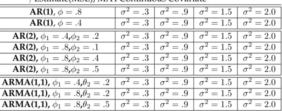
exposure data for a 7-day moving average by id. . . 52 2.6 30 Unique IDs - This table represents the initial values chosen for the simulation

study. For each correlation structure, AR(1), AR(2), and ARMA(1,1), the corre-lation coefficient, moving average coefficient, and variance were needed. Each scenario produced 5 data sets. . . 78

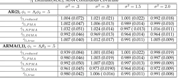
2.7 Small Deviations from AR(1) for 4-day Moving Average - This table represents the parameter estimates for a 4-day moving average from 5 separate linear mixed model using simulated data from the reduced, imputed, and true data sets. Linear mixed mean models were conducted for 200 iterations. The subsequent estimates were aggregated into means with accompanying MSE. Each model included one continuous covariate for weekend. All of the simulation standard errors are <

(15)

2.8 Large Deviations From AR(1) for 4-day Moving Average - This table represents the parameter estimates for a 4-day moving average from 5 separate linear mixed model using simulated data from the reduced, imputed, and true data sets. Linear mixed mean models were conducted for 200 iterations. The subsequent estimates were aggregated into means with accompanying MSE. Each model included one continuous covariate for weekend. All of the simulation standard errors are <

0.019. . . 79 2.9 Small Deviations From AR(1) for 7-day Moving Average - This table represents

the parameter estimates for a 7-day moving average from 5 separate linear mixed model using simulated data from the reduced, imputed, and true data sets. Linear mixed mean models were conducted for 200 iterations. The subsequent estimates were aggregated into means with accompanying MSE. Each model included one continuous covariate for weekend. All of the simulation standard errors are <

0.036. . . 80 2.10 Large Deviations From AR(1) for 7-day Moving Average - This table represents

the parameter estimates for a 7-day moving average from 5 separate linear mixed model using simulated data from the reduced, imputed, and true data sets. Linear mixed mean models were conducted for 200 iterations. The subsequent estimates were aggregated into means with accompanying MSE. Each model included one continuous covariate for weekend. All of the simulation standard errors are <

0.036. . . 80 3.1 Health effects estimates forαb andωb . . . 94

3.2 A(top left), B(bottom left), C(top right), D(bottom right): This table represents the parameter estimates and errors for the confirmatory factor analyses (CFA) models conducted on simulated data. Generalized linear models were conducted for 1000 iterations. The subsequent estimates were aggregated into medians. Each model included no covariates. . . 109 3.3 A(top left), B(bottom left), C(top right), D(bottom right): This table represents the

parameter estimates and errors for the confirmatory factor analyses (EFA) models conducted on simulated data. Generalized linear models were conducted for 1000 iterations. The subsequent estimates were aggregated into medians, and95%CI’s. Each model included no covariates. . . 110 3.4 A(top left), B(bottom left), C(top right), D(bottom right):This table represents the

parameter estimates and errors for the confirmatory factor analyses (PCA) models conducted on simulated data. Generalized linear models were conducted for 1000 iterations. The subsequent estimates were aggregated into medians, and95%CI’s. Each model included no covariates. . . 111 3.5 A(top left), B(bottom left), C(top right), D(bottom right):This table represents the

parameter estimates and errors for the two-stage hierarchical regression models conducted on simulated data. Generalized linear models were conducted for 1000 iterations. The subsequent estimates were aggregated into medians. Each model included no covariates. . . 111

(16)

3.6 This table represents the parameter estimates and errors for the 2-stage ”overlap” models conducted on simulated data. Generalized linear models were conducted for 1000 iterations. The subsequent estimates were aggregated into medians, and

95%CI’s. Each model included no covariates. . . 126

3.7 This table represents the parameter estimates and errors for the 2-stage ”no-overlap” models conducted on simulated data. Generalized linear models were conducted for 1000 iterations. The subsequent estimates were aggregated into medians, and

(17)

Acknowledgments

To begin, I would like to thank God for guiding my steps during the pursuit and completion of the doctoral program. At each celebration and each adversity, I have felt God’s presence by always placing me in the right environment and among the best people.

There have been a number of key figures that have been instrumental in my devel-opment as a researcher whom I would like to acknowledge. I truly had a ”dream team” of advisors. Through their concerted efforts and expert tutelage, I was able to learn and progress. I would like to recognize and thank my advisor, mentor, and professor, Brent Coull. Of his many genuine qualities I truly appreciated his warmth and ease. I always felt challenged but equally supported through course work , research, and the job search. He was always welcoming, available and un-derstanding which were irreplaceable qualities. I would like to thank Dr. Diane Gold for all of her encouragement throughout my time in Boston. Her expertise helped me to realize the importance of the work and how it can be used to aid real people. To Dr. Paul Catalano, thank you for your ideas, endless energy, and optimism which helped me to refine my statistical thinking and lift my spirits. In addition to my committee, I was lucky enough to have two academic advisors Pro-fessor Michael Hughes and ProPro-fessor Louise Ryan each of whom always showed the utmost confidence and faith in me.

Thank you to the invaluable staff in the Biostatistics department who kept me mov-ing in the right direction. They were able to act as a surrogate family for me since I was far from home. Thank you to Aunt Jelena Follwieller, Aunt Vickie Beaulieu, Aunt Phoebe Hackett, and my sister Rachel Boschetto. Lastly, I would like to thank Sabrina Toomer for her generosity and love. She always treated me like family and took care of me when I needed it-thank you so much.

Thank you to my many friends who shared this educational endeavor and toast to our successes and continued life long friendship. Thank you Binta Beard for hold-ing me down, your sacrifices and love will be valued forever. To Loni Phillip, Matt

(18)

Austin, Alane Izu, Shannon Stock, Roland Matsouaka, Alisa Stephens, Christina McIntosh, and Linda Valeri thank you so much for your friendship. Thank you to Ellen ”Kittie” Richardson and Ronald ”Kuda” Mills for your love and encourage-ment. I needed all of you in order to be successful so I am happy to share this with you.

Most importantly, I would like to thank my family. To my loving parents Dr. Aguibou Mouke Yansane and Maryam Cire Fofana, thank you for your love and support throughout my entire life. Each of you worked tirelessly to ensure that I would become a man who is loving and of good moral character. I hope that I have made you proud and been the blessing in your lives as you have been in mine. My sister, Kadidja Didi Mouke Yansane, I have always admired your courage, strength, and willingness to love. Thank you for always being there with your hu-mor, kind words, advice, and love. Lastly, I dedicate this dissertation to the mem-ory of my grandparents, Sekou Fofana and Aisha Cisse Fofana who passed away before the completion of my work. I was always in their thoughts and prayers, save a place in heaven.

(19)

Distributed Lag Path Analysis: Cardiovascular Effects

of Ambient Air Pollution

1

Alfa I. Yansan´e,

2,3

Diane R. Gold,

1,4

Paul J. Catalano,

1

Brent A.

Coull

1

Department of Biostatistics, Harvard School of Public Health

2

Department of Environmental Health, Harvard School of Public

Health

3

Department of Medicine, Brigham and Women’s

Hospital/Harvard Medical School and

(20)

1.1

ABSTRACT

Epidemiological studies have consistently demonstrated that elevated levels of particulate matter (PM) are associated with increased mortality and morbidity. Further studies have demonstrated a consistent increased risk for cardiovascular events such as myocardial infarction, stroke, cardiac arrhythmia, atherosclerosis, and angina (Mittleman et al. 2000; Rich Q, 2005; Dockery et al., 2005; Berger et al., 2006). In spite of prior evidence linking air pollution to these adverse health outcomes, the underlying causal, physiological, and biological pathways are less understood. The purpose of this article is to model and identifying the mechanis-tic pathways of effects by conducting a path analysis within a structural equation framework. This approach corresponds to jointly fitting two generalized additive distributed lag health outcome models, such that inferences on the health effects can be determined through direct and indirect pathways. We compare the perfor-mance of our approach in estimating the health effects ( changes in cardiovascular outcomes) to that of an existing approach of modeling the outcomes separately. Simulation results and subsequent data analysis suggest that the proposed dis-tributed lag path analysis are effective in simultaneously estimating the health effects from direct and and indirect path while conventional methods can not. We employ the proposed methods in the analysis of an Exposure, Epidemiology, and Risk Program study that investigates the effects of particulate air pollution

(P M2.5) on ST-Segment depression, T-wave alternans (TWA), and heart rate

(21)

1.2

INTRODUCTION

Epidemiological studies have consistently demonstrated that elevated levels of particulate matter (PM) are associated with increased mortality and morbidity. Further studies have demonstrated a consistent increased risk for cardiovascular events such as myocardial infarction, stroke, cardiac arrhythmia, atherosclerosis, and angina (Mittleman et al. 2000; Rich Q, 2005; Dockery et al., 2005; Berger et al., 2006). In spite of prior evidence linking air pollution to these adverse health outcomes, the underlying causal, physiological, and biological pathways are less understood. Identifying these mechanistic pathways will allow scientists, researchers, and medical professionals to become more informed and thus effec-tively focus medical interventions and treatments.

One of the primary objectives of PM research is the assessment of the health ef-fects related to specific types of air pollution. Particulate matter, sulfur dioxide, oxides of nitrogen, carbon oxides, and ozone have each been shown to be both chronic and acute contributors to adverse effects on human health (Brook et al. 2004). The scientific interest of this paper is to explore the relationship between particulate air pollution and a measure of cardiac electrical instability, T-wave al-ternans (TWA). Further, this study seeks to explore whether pollution leads to TWA through causing autonomic dysfunction, measured as a reduction in heart rate variability (HRV). We hope to jointly model these phenomena to understand interrelationships between the separate cardiac outcomes so that the effects of ex-posure can be decomposed into direct and indirect effects (via other outcomes). Investigations looking at the health effects of air pollution recognize that a health outcome can be affected by exposures experienced either at the time the outcome is measured or during some time previous to the health assessment. Accounting

(22)

for both contemporaneous and lagged effects would give a more well rounded as-sessment of pollution and help to avoid exposure misclassification biases. Some studies have shown that pollutant exposures measured at different lengths of time have will have a varied impact on the outcome (Chuang et al. 2008). Further, the relevant time windows may change depending on the outcome. Therefore, ap-propriate models must account for both immediate and lagged exposure effects, repeated measures, smoothed terms, and missing values. In this paper, we pro-pose to develop methods that allow one to examine pathways of effects, when the lagged effects of exposure are potentially of interest. We plan to use distributed lag models merged within a structural equation framework to examine the rela-tionship between air pollution and different electrical cardiac outcomes that are known precursors to cardiovascular events.

At present, existing analyses attempt to consider temporal resolution through the use of moving averages. The ”moving average” method of analysis calculates ex-posure concentrations over various pre-specified intervals of time. Hence, each model produces one effect estimate for the respective moving average. In this modeling scheme the pollutant could be modeled as a linear or smoothed term depending the assumed relationship. It has been recognized in the literature that the effects of pollution are sensitive to the length of the moving averages used for exposure measures so effects may not be fully captured.

Another issue arises when attempting to consider multiple cardiac endpoints si-multaneously, because different lags of exposure may be most relevant for the dif-ferent outcomes. This means that each endpoint has its own pivotal time interval where the adverse health effects may be the highest in magnitude. If all of the models used the same time interval and resolution, it is possible that effects may

(23)

be seen in one outcome but not others. In this paper, we propose a path anal-ysis that jointly fits two or more distributed lag models using the pollutants as exposures and the measures of cardiac electrical instability as outcomes. Modeling these outcomes jointly will allow for both direct and indirect effects to be estimated at varying time lags.

The data that motivates the proposed research comes from three analyses con-ducted through the Exposure, Epidemiology, and Risk Program in Boston on the effects of particulate air pollution (particulate matter, black carbon, carbon monox-ide, ozone, nitrogen dioxmonox-ide, and sulfur dioxide) on T-wave alternans and heart rate variability. Harvard researchers have conducted a number of regression anal-yses using moving averages of exposure and these outcomes. Pollutants were mea-sured from a central site while the heart outcomes were calculated by a personal monitor at half hour intervals. There has been some exploration of potential bi-ological pathways for this relationship such as; Direct paths through the cardio-vascular system, blood, and lung receptors, or indirect paths through pulmonary oxidative stress and inammatory response (Brook et al. 2004). In order to explore the intermediate effects and their inter-relationship with other outcomes, a path-way model can be implemented and we will introduce and derive approaches for the implementation of such a model. Our proposed work seeks to help elucidate the electro-physiological mechanism to complement the existing research.

This paper is organized as follows: Section 1.3 describes in detail the design and data from a study evaluating the effects of particulate air pollution on electrical cardiac instability. Section 1.4 presents the distributed lag model and subsequent pathway model, while Section 1.5 discusses the direct and indirect effects of expo-sure. Section 1.6 gives a short treatment of the Bayesian approach to estimation

(24)

and Section 1.7 presents a simulation study to examine the effectiveness pathway analytic model, compared to the moving average approach. Section 1.8 demon-strates an application of the distributed lag pathway model (DLPWM) to analyze the afore mentioned study from Exposure, Epidemiology, and Risk Program and finally in Section 8 we discuss our findings along with implications for future path analyses.

1.3

DATA DESIGN

1.3.1

Data Collection

The study population consisted of a recruited panel of patients with documented coronary artery disease from the greater Boston area. Specifically, subjects were re-cruited within route 495 (the outer most boundary of the greater Boston metropoli-tan region) and a 40 km radius from the central pollution monitoring site. Each subject had experienced a percutaneous coronary intervention for an acute coro-nary syndrome or for worsening stable corocoro-nary artery disease. In each study, patients were excluded with atrial fibrillation and left bundle branch block (LBBB) because of the intent to evaluate heart rate variability and ST-Segment as outcomes. Further exclusions included patients who had bypass graft surgery within the last 3 months because accurate interpretations of the T-wave and ST-Segment would have been compromised. Other exclusions were active smokers, drug or alcohol abuse problems, and those with psychiatric illness. Subjects received a home visit within 2 to 4 weeks after the hospital discharge, followed by 3 additional visits at approximately 3 month intervals. There were 48 subjects yielding 129 person-visits with 6135 observations. Each patient had approximately 48 half-hour ST-segment,

(25)

T-wave alternans, and heart rate variability (HRV) measurements taken, which were linked with air pollution measurements at corresponding times.

The outcomes were measured using 24 hour 3 lead Holter ECG monitoring and the electrodes were placed in modified V5 and VF positions. In the subsequent visits, patients were given a follow-up questionnaire regarding cardiac and respiratory symptoms, and medication use. They later received 24-hour Holter monitoring. Ambient concentrations of particulate air matter with aerodynamic diameter less

than 2.5µm (P M2.5) and black carbon (BC) were measured at the central

moni-toring site located on the roof of Countway Library, Harvard Medical School, in

downtown Boston, MA.P M2.5 concentrations were measured using Tapered

Ele-ment Oscillation Microbalance (TEOM, Model 1400A, Rupprecht and Pataschnick,

Albany, NY). Ambient BC was measured using an aethalometer. P M2.5 and BC

concentrations were summarized in half hour intervals with analysis based on half

hour, 12 hour lagged, and cumulative exposures. Indoor P M2.5 and BC

measure-ments were also taken. O3, SO2, and CO measurements were obtained using state

monitoring sites in Boston, MA.

1.3.2

Single Outcome Analyses

A first analysis assessed the relationship between heart rate variability (HRV) and ambient air pollution among the post coronary event patients (Zanobetti et al. 2009). Authors explored this relationship because reduced HRV has been linked to increased risk of myocardial infarction, increased mortality in patients with heart failure, and is a marker for fatal ventricular arrhythmia (Gold et al. 2000; Task Force of the European Society of Cardiology the North American Society of Pac-ing Electro-physiology, 1996). HRV was measured usPac-ing four different metrics;

(26)

standard deviation of normal-to-normal heart beat intervals(SDN N)and square root of the mean of the squared differences between adjacent normal RR intervals (r-MSSD), high frequency (HF), and total power (TP). The smaller the standard de-viation in the RR intervals corresponded with lower HRV measures. The authors used generalized additive models to control for confounding, which allowed for the covariates to have non-linear effects on outcome. For both r-MSSD and HF, the

authors found significant negative associations with P M2.5 and BC. There was a

tendency for the stronger r-MSSD associations to occur at longer averaging times. The second analysis of this study was to explore the relationship between partic-ulate pollution and T-wave alternans (Zanobetti et al. 2009). T-wave alternans (TWA) are periodic beat to beat variations in the amplitude of the T-wave in an electrocardiogram (ECG). It is most often measured in patients who have had my-ocardial infarctions or other heart damage to see if they are at high risk of devel-oping a potentially lethal cardiac arrhythmia. The shape of the T-wave could be a key indicator of cardiac health and mortality (Nieminen et al. 2007; Stein et al. 2008). For example, inverted or negative T-waves can be a sign of coronary is-chemia, whereas tall or tented symmetrical T-waves may indicate hyperkalemia. TWA is also a marker of cardiac electrical instability measured as differences in the magnitudes between adjacent waves. Increases in the previous 1 to 12 hour

av-eraged ambientP M2.5 and BC were associated with increases in TWA, with peak

cumulative effects in between 6 and 12 hours. The authors’ estimated that for a

1 unit increase in 6 hour averagedP M2.5 there was an increase of 1.7%(0.6,2.7)in

(27)

1.4

MODEL AND NOTATION

1.4.1

Modeling Framework

An alternative to separate ”moving average” models is the distributed lag model (DLM). Distributed lag models generalize the single time point or moving average models because they estimate differential air pollution effects for all lagged time points simultaneously, rather than from separate models. Our data have been col-lected so that measurements for each pollutant have been colcol-lected for 48 separate half-hour time lags along with the corresponding electrical cardiac instability out-comes at those times. Therefore the data are suited for distributed lag modeling framework.

We begin with a generalized additive distributed lag model that adjust for lagged exposures, linear and non-linear effects of confounders, and random subject ef-fects, Yit =η0+ q X l=0 βlxi,t−l+ d X j=1 fj(sitj) +γTxit,linear+Ui+it (1.1)

where q is the the number of lagged time points.Xitis the half-hour pollution

mea-sure of subject i at time t (P M2.5) (Zanobetti et al., 2000).Yitis the outcome measure

of subject i at time t. Theit is the error of subject i at time t and is normally

dis-tributed with zero mean and constant varianceσ2

. TheUiis the random coefficient

due to subject i also with mean zero and varianceσ2

u. The vectorxit,linear is a

vec-tor of variables modeled linearly andγ represent the effect estimates. The overall

impact of a unit change in in exposure over q days is given byΣq_t₌₀βl(Schwartz et

(28)

or spline function of l. For eachβlthere were three different options utilized. They

will be represented by the following equations. Option 1(Parametric): βl = p X r=1 τrlr where0≤l≤q

Option 2 (Thin-Plate Spline)(Crainiceanu et al., 2005):

βl = 2 X r=1 τrlr+ K X k=1 νk|l−κk|3 where0≤l≤qand

Option 3 (Truncated Spline):

βl= p X r=1 τrlr+ K X k=1 νk(l−κk)p+ where0≤l≤qand (l−κk)p₊ = ( (l−κk)p if l ≥κk 0 if l < κk ,

whereκ1, . . ., κK is a set of K distinct numbers between 0 and q. βl is a piecewise

pth degree polynomial in l, with join points (knots) at theκk. Theνkare coefficients

associated with the basis function(l−κk)

p +.

(29)

(Carroll et al., 2003): fj(sitj) = p X c=1 αj,cscitj+ Kj X k=1 ωj,k(sitj −κj,k)p+

Thesijtis the confounder variable for theithsubject, thejth variable modeled as a

smooth function at time t. Theαj,c is the coefficient forjth smoothed term. While

the ωj,k are the coefficients corresponding to the basis function (sitj − κj,k)p₊ for

thejth _{smoothed variable. Each smoothed term can be expressed in the form of a}

linear mixed model with both fixed and random terms.

1.4.2

Distributional Assumptions

Model (1.1) can be simplified through matrix representations below:

Y =XLagτ +ZLagu+ Pd j=1Xsmooth,jαj+ Pd j=1Zsmoothwj+XLinearγ+ τ = [η0, τ0, τ1, . . . , τp] T α= [α0, α1, . . . , αp]T u= [U1, U2, . . . , Um]T ν = [ν1, ν2, . . . , νK]T wj = ω1, ω2, . . . , ωKj T γ = [γ1, γ2, . . . , γb] T

(30)

of distinct subjects such that 1 ≤ i ≤ m. , and let ni represent the number of

observations at time t. By concatenating the model further and using the fact that the spline coefficients can be modeled as random effects, the above equation can be reduced to the simple mixed model (1.2) in the following form:

Y1 =

XLag XSmooth XLinear       τ α γ       + ZLag ZSmooth    u w   + (1.2) Y1 =Xβ1+Zb1+ (1.3) Cov    b   =          σ2 uI 0 0 0 0 σ2 νI 0 0 0 0 σ2 ω,jI 0 0 0 0 σ2 I         

The form of this model could be applied to other outcomes, for example ST seg-ment. The model would be analogous to the one above including the same con-founders but with a different outcome.

Y2 =Xβ2+Zb2+, (1.4)

1.4.3

The Pathway Analytic Model

Path analysis can be used to test theoretical models that specify causal relation-ships between a number of observed variables (Hatcher, 1994). Structural

(31)

equa-tion models (SEM’s) are a set of flexible models that enable the modeling of mul-tivariate data for path analyses. SEM’s can handle both simple and hierarchical modeling structures (Sanchez et al., 2005). An essential tool for SEM’s is the path diagram or directed acyclical graph (DAG) that details causal relationships graph-ically. Each variable is represented by its own box. Single-headed arrows represent causal relationships between two different variables. In Figure 1.1, the x variable represents the independent variable or antecedent variable, predicted to precede and have a causal effect on y. The y box represents the consequent variable or the dependent variable. The straight, single-headed arrow is generally used to repre-sent a directional causal path in a path diagram while also detailing the statistical model that describes the relationship. The z variable can be considered an inter-mediate (mediator) variable because it is on the causal pathway from x to y and it is caused by x.

Through normal likelihood theory, estimation of parameters, confidence intervals, and p-values can be calculated. Standard approaches to pathway analysis usually make the assumption that the variables of interest are normally distributed. Sub-sequently, direct paths have point and interval estimates while indirect paths are the product of the estimate of the independent variable to the intermediate variable and that for the association between estimate of the intermediate variable to the de-pendent variable. In the normal theory case, these parameters could be estimated using to least squares equations. The following example is a simple illustration of the modeling scheme.

Let y be the outcome variable, x be the independent variable, and z be the

intermediate variable whereby θ2 denotes the linear association between x and y,

(32)

between z and y. The DAG for the model is as follows: z =θ0+xθ1+ez (1.5) y=θ00+xθ2+zθ3+ey (1.6) ..   θ1  θ3    θ2        x        y        z 

Figure 1.1:General Form

By substituting the value z from equation (1.5) into equation (1.6) we have the

resulting equation that allows one to estimateθ1θ3andθ2.

y =θ00+θ0θ3+xθ2+xθ1θ3+ezθ3+ey (1.7)

This method is effective when the variables are normally distributed (Gajewski et al., 2006). There is also the question of calculating the appropriate standard errors

using this method because the standard errors forθ1 andθ3 are correlated.

There-fore, there is a natural congruence between the directed acyclical graph (DAG) and its corresponding model.

Extending this basic conceptual structure using generalized distributed lag mod-els we present Figure 1.2 below as a potential directed acyclical graph (DAG). We

(33)

propose that the GADLMs below are an accurate reflection of the DAG and will be able to estimate the direct effects of pollutant on T-wave alternans as well as the indirect effects through the intermediary HRV. Equation (1.8) represents a model

that estimates the direct effects of the exposure(xit)on outcome 1(Y1,it)where the

β1,l are the parameters of interest. While model (1.9) estimates the effect of

expo-sure (xit) on the second outcome (Y2,it)through the intermediary (Y1,it). The β2,l

are the distributed lag function for the direct effects between T-wave alternans and

the pollutant. Theϕlrepresents the coefficient of the intermediate outcome(Y1,it).

Hence, through the SEM framework model (1.9) accounts for multiple endpoints on the causal pathway and yields interpretable direct and indirect effects.

..

Exposure T-‐Wave Alternans HR Variability

Figure 1.2:DAG for Air pollutant exposure

Y1,it =η1,0+ q X l=0 β1,lxi,t−l+ d X j=1 fj(sitj) +γ1Twit+U1,i+1,it, (1.8) Y2,it =η2,0+ q X l=0 β2,lxi,t−l+ q X l=0 ϕlY1,i,t−l+ d X j=1

(34)

1.5

DIRECT AND INDIRECT EFFECTS

1.5.1

Interpretation

In a broad sense, the relationship between an exposure of interest and an outcome can be singular or multifactorial. We are interested in quantifying the relationship through detailing the magnitude, direction, and causal pathway. A direct effect is defined as a link between an exposure and outcome. Given the previous DAGs, the direct effects are represented by a single arrow with no intermediaries. On the other hand an indirect effect is the link between an exposure and outcome that con-sist of intermediaries on the pathway. Therefore, more than one arrow is needed to describe the relationship. This is significant because researchers will be able to explore whether the effects of a pollutant can be seen directly or indirectly through an intermediary. This will illuminate many questions regarding the electrophysio-logical pathway between pollutants and electrical cardiac outcomes as well as test for interrelationships. For example, in our current data set, HRV precedes TWA on the electro-physiological pathway and researchers would like to investigate the scientific trail where the pollutants are the most influential.

Using figure 1.2 as the model DAG, we estimate the direct effect between outcome

(TWA) and the exposure (pollutant) with a set of parameters β2,l represented by

a smoothed curve, and the indirect effects between the outcome variable and the exposure through the mediating variable is represented by another curve proven below: Y1,it =η1,0+ q0 X l0₌₀ β1,l0x_i,t₋_l0+ d X j=1 fj(sitj) +γ1Twit+U1,i+1,it, (1.10)

(35)

Y2,it =η2,0+ q X l=0 β2,lxi,t−l+ q X l=0 ϕlY1,i,t−l+ d X j=1

gj(sitj) +γ₂Tw1,it+U2,i+2,it (1.11)

Now we substitute equation (1.10) into equation (1.11) and rearrange the terms.

Y2,it = η2,0+ q X l=0 β2,lxi,t−l+ q X l=0 ϕl " η1,0+ q0 X l0₌₀ β1,l0x_i,t₋_l0₋_l+· · ·+₁_,i,t₋_l, # + d X j=1

gj(sitj) +γ2Tw1,it+U2,i+2,it

Since we are only interested in the direct and indirect effects of exposure and their

interpretations we will use the following as our model of interest where[∗∗]

repre-sents the other terms/confounders in the model after some.

Y2,it = " _q X l=0 β2,lxi,t−l+ q X l=0 q0 X l0₌₀ ϕlβ1,l0x_i,t₋_l0₋_l # + [∗∗]. = " q X l=0 β2,lxi,t−l+ q+q0 X k=0 β_k∗xi,t−k # + [∗∗]

The β2,l parameters represent the set of direct effects of lagged exposure on our

outcome and

whereβ_k∗ = P

l+l0₌_k[ϕlβ1l0]represents the indirect effect of the lagged exposure on

(36)

1.6

ESTIMATION

Standard distributed lag models (DLM’s) could be fit using maximum likelihood methods by including all covariates in a generalized linear-mixed model. ML methods require large sample sizes for asymptotic optimality of the resulting ML estimators. Since we have 48 lagged exposures to be included in the model, these methods may not be optimal. Further, the number of parameter estimates increases when conducting the pathway analyses to account for the new effects.

We propose a non-informative Bayesian approach to modeling these distributed

lag data. We wish to estimate the effect of P M2.5 on two separate cardiovascular

outcomes simultaneously. The estimates will be represented byτr forr = 1, . . . , p.

Non-informative priors are proposed for each parameter so that the estimates are

primarily data driven. Eachτ is distributed as follows:

τ ∼N(0,Ψ)

Where Ψ = 10,000. An informative approach could have been done as well but

more data from previous studies would have been needed.

1.7

SIMULATION STUDY

We conducted a simulation study to examine the effectiveness of DLM pathway model to estimate the changes in TWA and HRV. We would also like to perform a direct comparison of estimates between a moving average, parametric, and semi parametric approaches. The intended outcomes, the lagged exposure, and the

(37)

co-efficients must be simulated under varying assumptions in order to get a complete picture of the model effectiveness while decomposing the exposuoutcome re-lationship. We began with 50 subjects yielding 100 person-visits with 5000 total observations. There were also 50 measurements taken for each of the 100 subjects and 50 lagged time-points created to mimic those in the real data.

1.7.1

Simulating Lagged Data

To simulate exposure, we generated 50 P M2.5 exposure variables lagged by half

hour intervals fromX∼N(µx,Σx). We assumed,

Σx=             σ2 x ρ ρ2 . . . ρ49 ρ σ2 x ρ . . . ρ48 ρ2 _ρ _σ2 x . . . ρ47 .. . ... ... . .. ... ρ49 ρ48 ρ47 . . . σ_x2             ,

whereρ = 0.4to reflect the fact thatP M2.5 measurements taken at closer intervals

are more highly correlated. σ2_x = 1 and µx = 5 were taken from averages in the

real data.

1.7.2

Simulating Outcome 1

Next, we picked initial values under varied conditions forτ that were also chosen

based estimates from the models of the real data. Each βl was then calculated

(38)

polynomial spline. These values were needed to simulate the direct effect between

Y1(HRV) andX(P M2.5). Y1 was simulated from the following distribution:

Y1|X, β1 ∼N( q0 X l0₌₀ β1,l0x_i,t₋_l0, σ2 y1)

1.7.3

Simulating Outcome 2

Our next task was to simulateY2 which reflects the indirect effectP M2.5 and TWA.

In addition to choosing initial values forτ2, initial values forϕwere designated as

they represent the intermediary effects between HRV and TWA. Since HRV only acts on TWA for a short period of time, the lagged relationship between HRV and TWA only spanned 2 time points. Although for thoroughness in understanding we conducted simulation with 6 intermediary time points. The intermediary time

point values denoted by the variableϕland given by the function,ϕ[i] = 0.1−.001i2

fori= 1, . . . ,6. Y2 was then simulated from the following distribution:

Y2|Y1, β2 ∼N( q X l=0 β2,lxi,t−l+ q X l=0 ϕlY1,i,t−l, σy22)

1.7.4

Simulation Path Model

Table 1.1 gives the assumed true values used for each simulated scenario. They represent distinct, biologically plausible combinations of distributed lag functions

for HRV and TWA. Using the values of τ in table 1.1, the corresponding health

effect estimatesβlare calculated. Next, theX, Y1, andY2)values are generated for

(39)

path model only included lagged exposure variables and lagged Y2 values. The

form of the simulated path model is as follows:

Y1,it =η1,0+ q0 X l0₌₀ β1,l0x_i,t₋_l0 +U₁_,i+₁_,it, (1.12) Y2,it =η2,0+ q X l=0 β2,lxi,t−l+U2,i+2,it (1.13) where βl = Pp

r=1τrlr. Both the parameters and hyper parameters were given the

following non-informative priors.

τ ∼N(0,100000) Ui ∼N(0, σ2u) σ2_u ∼IG(0.01,0.01) σ2_y ∼IG(0.01,0.01)

For each data set, the posterior distribution is estimated using MCMC methods using 10,000 iterations and subsequently keeping 1,000 posterior values. The mix-ing of each model is checked visually by the trace plots to see if convergence was achieved. Next, the median and point-wise 95% credible interval of each lagged time point are calculated for each of the 100 sets of posterior effect estimates.

(40)

1.7.5

Simulation Results

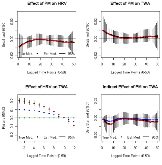
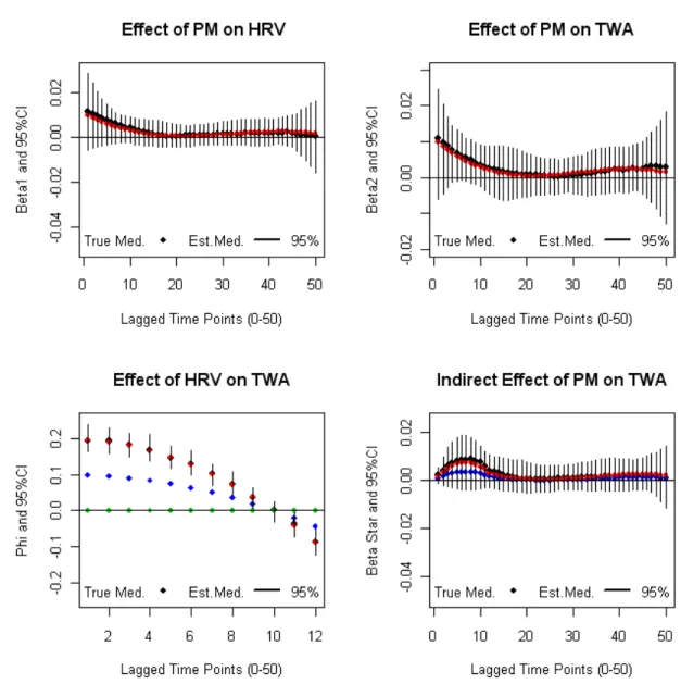
Each simulated pathway model will be designated by 4 output graphs where the X-axis represents the lagged time points and the Y-axis is the magnitude of the pos-terior effect estimate. Each plot includes a true (red curve) and estimated (black

curve) distributed lag function and95%confidence bands (black) for the

relation-ship between: 1) PM and HRV (β1,l), 2) PM and TWA (β2,l), 3) HRV and TWA

(ϕl), and 4) Indirect Effect of PM on TWA through HRV(βl∗). The blue curve in the

3rd position plot represents a reduced setting on the magnitude of the relationship between HRV and TWA. The blue curve in the 4th position gives the indirect

asso-ciation ofP M2.5on TWA through HRV for the afore mentioned reduced setting.

Figure 1.3 represents the first simulation setting model due to its biological pattern.

In the literature we see that HRV has a negative relationship withP M2.5and TWA

has a positive relationship withP M2.5. For this simulation scenario we note that

the estimated distributed lag function quite accurately estimates the true DLF and

is also within95%credible limits in all 4 graphs.

The pathway model for the first simulation shows that the relationship between

P M2.5 and HRV is negative. Early lags reflect the highest effects while later lags

move towards 0. The relationship betweenP M2.5 and TWA is positive with most

of the effect occurring at earlier lags as well. The distributed lag function for the

indirect effects (β_l∗) are almost identical to the distributed lag function between

P M2.5 and HRV except for the first 12 time points. As we would expect, the

indi-rect effect depends on the magnitude of the distributed lag function for the

rela-tionship between HRV and TWA given byϕl, and our procedure is able to

appro-priately separate out these direct and indirect effects. Other simulation scenarios were completed and the conclusions were similar.

(41)

Model Initial-τ0 Initial-τ1 Initial-τ1 Initial-τ3 Model 1: HRV(τ1) -0.01 0.0011 -0.000041 0.00000043 TWA(τ2) 0.01 -0.0011 0.00004 -0.00000043 Model 2: HRV(τ1) 0.00 0.00 0.00 0.00 TWA(τ2) 0.01 -0.0011 0.00004 -0.00000043 Model 3: HRV(τ1) -0.01 0.0011 -0.000041 0.00000043 TWA(τ2) 0.0 0.00 0.00 0.00 Model 4: HRV(τ1) -0.01 0.0011 -0.000041 0.00000043 TWA(τ2) 0.001 -0.0005 0.00006 -0.000001 Model 5: HRV(τ1) 0.01 -0.0005 0.00006 -0.000001 TWA(τ2) 0.01 -0.0011 0.00004 -0.00000043 Model 6: HRV(τ1) 0.01 -0.00055 0.000041 0.000001 TWA(τ2) 0.01 -0.0011 0.00004 -0.00000043 Model 7: HRV(τ1) -0.001 0.00015 -0.000005 0.0000002 TWA(τ2) 0.01 -0.0011 0.00004 -0.00000043 Model 8: HRV(τ1) 0.01 0.0011 0.000041 0.00000043 TWA(τ2) 0.01 -0.0011 0.00004 -0.00000043

Table 1.1:This table represents the initial values chosen for the simulation study. For each model,

4 initial values were chosen for both HRV and TWA. Each model corresponds to a distinct plausible distributed lag function.

1.8

DATA ANALYSIS

1.8.1

Prior Elicitation

Given the motivating heart data, DLMM models were fit using the same con-founders as the initial analysis described in Section 1.2. The following model was used for this analysis:

Y1,it =η1,0+ q0

X

l0₌₀

(42)

..

Figure 1.3:Model 1-Regular HRV; Regular TWA

where: β1,l = p X r=1 τrlr where0≤l≤q

We used the above parametric parameterization of β1,l for p=2, 3, and 4 which

corresponds to quadratic, cubic, and quartic single pollutant models. We also at-tempted to use the ”Thin-plate spline” and ”Truncated spline” parameterizations

(43)

of the week as indicator variables while average heart rate, mean temperature, hour of the day using quadratic effects. Quadratic effects were chosen for these variables because univariate generalized additive models were run and quadratic effects seemed to be a plausible approximation. Lastly, numerical date was con-trolled for using the following parameterization:

date1 = sin(2∗π_T∗date), date2 = cos(2∗_Tπ∗date)

To conduct this Bayesian analysis we utilized Markov Chain Monte Carlo meth-ods MCMC to estimate the parameters for the DLM using the R statistical pack-age (The Comprehensive R Archive Network: http://cran.r-roject.org/). The ”R2Winbugs” function was used so that Winbugs could be accessed within the R platform (Crainiceanu et al., 2005). Since our model was fit in the Bayesian setting, we assigned non-informative priors for the model parameters.

τ ∼N(0,100000) ui ∼N(0, σ2u) ωj ∼N(0, σ2ωj) σ2_u ∼IG(0.01,0.01) σ_ω2 j ∼IG(0.01,0.01) σ2_y ∼IG(0.01,0.01)

Each model was run using a burn-in period of 20,000 iterations. The convergence of each estimated parameter was checked by visual inspection of the trace plots. We kept 5,000 posterior samples thinned by 5 for each of the 49 lagged estimates.

(44)

The total effect of a particular pollutant over q hours was calculated by summing over the lagged coefficients given by the posterior samples. This yielded 5,000 posterior samples of the total pollutant effect over 24 hours so that medians and confidence intervals could be produced.

1.8.2

Health effects analysis

Heart Rate Variability

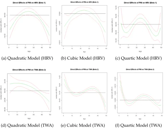
Figure 1.4 is a plot of the distributed lag function for the relationship between HRV

(measured as r-MSSD) andP M2.5. Each graph represents a quadratic, cubic, and

quartic parameterization of this relationship. Subject, day of the week, average heart rate, mean temperature, hour of the day, and were the included confounders.

Figure 4 reveals that the effect of P M2.5 on heart rate variability has a

curvilin-ear shape that is concave and the effect is mostly negative across the three model

versions. The overall impact of a unit change in P M2.5 over 48 lags (24 hours)

was associated with a -0.00872 (-0.013, -0.0049) reduction in HRV for the quadratic model, -0.0085 (-0.0124, -0.0046) reduction in HRV for the cubic model, and -0.0084 (-0.0124, -0.0042) reduction in HRV for the quartic model. This shows consistency across the parameterization. These results are consistent with the moving average results of Zanobetti et al. 2000.

T-wave alternans

Figure 1.4 also contains plots of the distributed lag function for the relationship

(45)

(a) Quadratic Model (HRV) (b) Cubic Model (HRV) (c) Quartic Model (HRV)

(d) Quadratic Model (TWA) (e) Cubic Model (TWA) (f) Quartic Model (TWA)

Figure 1.4:Top Row: SINGLE OUTCOME MODEL HRV - Each graph represents the DL function

of the relationship betweenP M2.5and HRV adjusting for subject, day of week, average heart rate,

mean temperature, hour of the day, and date. Bottom Row: SINGLE OUTCOME MODEL TWA -Each graph represents the DL function of the relationship betweenP M2.5and TWA adjusting for

(46)

parameterization of this relationship. Figure 5 reveals that the effect of P M2.5 on

TWA has a curvilinear shape that begins with a highly positive effect for early lags

and approaches zero for later lags. The overall impact of a unit change inP M2.5

over 48 lags (24 hours) was associated with a 0.0023 (0.00042, 0.00421) increase in TWA for the quadratic model, 0.0030 (0.0012, 0.0050) increase in TWA for the cubic model, and 0.0032 (0.0013, 0.0051) increase in TWA for the quartic model. Each

of the estimates show a significant and positive relationship between P M2.5 and

TWA-. Zanobetti et al., 2009 shows that with increasing moving averages, there is an increase in the TWA which means that the two approaches are in accord (See Appendix Figure 8).

1.8.3

Path Analysis

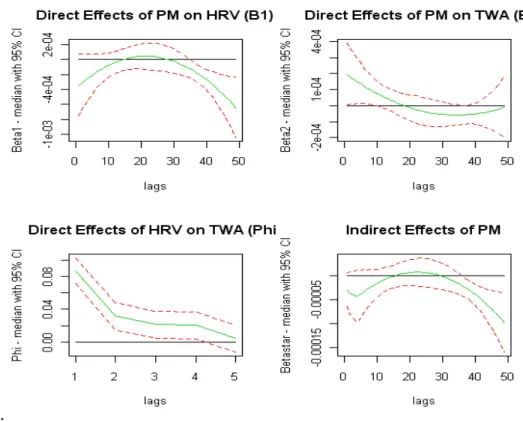
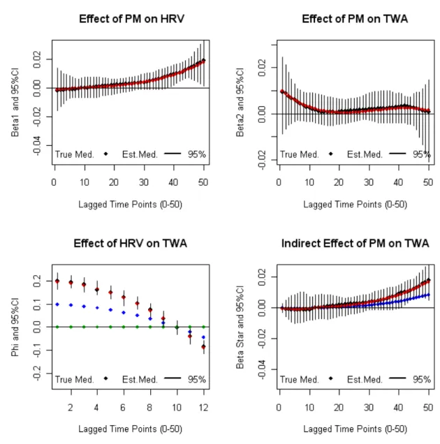
The path analyses in Figures 1.5, 1.6, and 1.7 reflect the real data from the Expo-sure, Epidemiology, and Risk Program in Boston. The outcomes of specific interest

are HRV (measured through r-MSSD) , TWA, and the exposure isP M2.5 just as in

sections 1.8.1 and 1.8.2. In the previous sections, the distributed lag models were used to show the univariate relationships between exposure and outcome control-ling for potential confounders. In the current section, the path models seek to estimate these effects simultaneously and in aggregate along with the inclusion of an indirect effect. The path model is included below:

Y2,it =η2,0+ q X l=0 β2,lxi,t−l+ q X l=0

ϕlY1,i,t−l+γ2Tw1,it +U2,i+2,it, (1.15)

(47)

..

Figure 1.5: QUADRATIC PATH MODEL - Clockwise : 1)P M2.5on HRV, 2)P M2.5 on TWA, 3)

P M2.5on TWA indirectly through HRV, and 4) HRV on TWA.

Y1,it =η1,0+ q

X

l=0

β1,lxi,t−l+γ1Twit+U1,i+1,it, (1.16)

In order for the path model to be fully implemented a lag structure needed to be

created for Y1,i,t−l (HRV). 4 lags were used to describe the relationship between

HRV and TWA because the largest effects were seen within that time. As a result of the creation of these new lags 4 observations per study id had to be removed. We also investigated 8 lags for the HRV vs.TWA relationship and the results were comparable. Figures 1.5 - 1.7 show the distributed lag function for the following

relationships in a clockwise fashion: 1)P M2.5on HRV, 2)P M2.5 on TWA, 3)P M2.5

on TWA indirectly through HRV, and 4) HRV on TWA. Each plot consists of a median posterior curve and a corresponding 95% credible interval. The distributed

(48)

..

Figure 1.6: CUBIC PATH MODEL - Clockwise : 1)P M2.5on HRV, 2)P M2.5on TWA, 3)P M2.5

on TWA indirectly through HRV, and 4) HRV on TWA.

lag functions in position 1) and 2) from each of the path models are similar in shape to their separate model counterparts respectively.

In Table1. 2 we see the overall estimated effects of the separate models juxtaposed with overall estimated effects of the pathway models. We found significant

asso-ciations between HRV andP M2.5 in both the separate and pathway models in all

cases, and the overall estimates were similar. All of the estimates show a negative

relationship whereby increases inP M2.5are associated with decreases in HRV.

Fur-ther, the distributed lag functions of the quadratic, cubic, and quartic path models

are similar. Significant associations were found between TWA andP M2.5 in both

the separate and pathway models in all cases as well. All of the estimates show

(49)

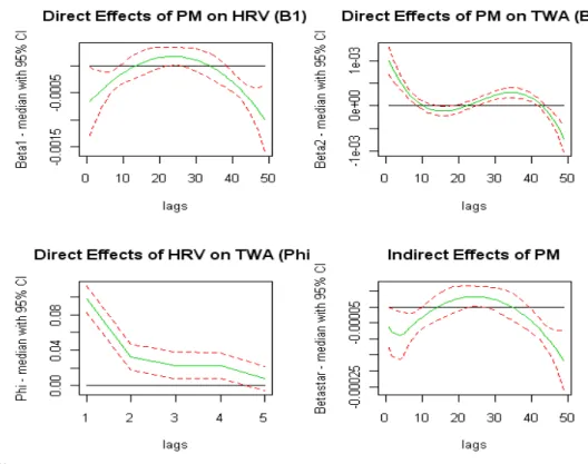
in-..

Figure 1.7:QUARTIC PATH MODEL - Clockwise : 1)P M2.5on HRV, 2)P M2.5on TWA, 3)P M2.5

on TWA indirectly through HRV, and 4) HRV on TWA.

creases in TWA. Once again, the distributed lag functions of the quadratic, cubic, and quartic path models are similar. The effect estimates from the separate models were attenuated by approximately 37-46% in comparison with the pathway model estimates for TWA. The direct and indirect effects are intrinsically included when conducting the single outcome models, which leads to the dimmed effect estimate. The indirect effects cannot be estimated in the separate models because they would not have been simultaneously done. The pathway model estimates a negative

overall effect for the indirect relationship between P M2.5 and TWA through the

intermediary HRV in the quadratic, cubic, and quartic cases. The overall impact of

a unit change inP M2.5 over 48 lags (24 hours) is associated with a -0.0086 (-0.0126,

(50)

Outcome Quad. Separate Model Est. and 95%CI Quad. Path Model Est. and 95%CI

HRV(β1,l): -0.00872 (-0.013, -0.0049)† -0.0086 (-0.0126, -0.0046)†

TWA(β2,l): 0.0023 (0.00042, 0.00421)† 0.0043 (0.0025, 0.0063)†

Indirect(β∗_{) :} _N/A _{-0.0014 (-0.0022, -0.00071)}_†

Outcome Cubic Separate Model Est. and 95%CI Cubic Path Model Est. and 95%CI

HRV(β1,l): -0.0085 (-0.0124, -0.0046)† -0.0085 (-0.0124, -0.0044)†

TWA(β2,l): 0.0030 (0.0012, 0.0050)† 0.0050 (0.0031, 0.0069)†

Indirect(β∗): N/A -0.0014 (-0.0021, -0.00065)†

Outcome Quartic Separate Model Est. and 95%CI Quartic Path Model Est. and 95%CI

HRV(β1,l): -0.0084 (-0.0124, -0.0042)† -0.0083 (-0.0124, -0.0042)†

TWA(β2,l): 0.0032 (0.0013, 0.0051)† 0.0051 (0.0032, 0.0070)†

Indirect(β∗): N/A -0.0015 ( -0.0023, -0.00070)†

Table 1.2: This table represents the parameter estimates from separate parametric distributed

lag models and the parameter estimates from the pathway models for 48 lags (24 hours). The intermediaryϕis 4 lagged time-points.†Denotes significance atα= 0.05.

for the quadratic, cubic, and quartic models respectively. The overall impact of

a unit change inP M2.5 over 48 lags (24 hours) is associated with a 0.0043 (0.0025,

0.0063), 0.0050 (0.0031, 0.0069), and 0.0051 (0.0032, 0.0070) increase in log(TWA)µV

for the quadratic, cubic, and quartic models respectively. Finally, the overall

indi-rect impact of a unit change inP M2.5 over 48 lags (24 hours) is associated with a

-0.0014 (-0.0022, -0.00071), --0.0014 (-0.0021, -0.00065), and -0.0015 ( -0.0023, -0.00070)

decrease in log(TWA)µV through HRV for the quadratic, cubic, and quartic

mod-els respectively. We see that the distributed lag function for the indirect effects mimics the the DL function for HRV except for the the first 6 time points.

This study provides evidence that exposure to ambient air pollution in the form

of P M2.5 increases cardiac electrical instability over a 24 hour period capturing

effects during sleep, morning hours, as well as normal activity. This finding offers a possible parsing of the mechanisms that lead to cardiac events.

(51)

1.9

DISCUSSION

In this paper, we considered methods to assess specific health effects ofP M2.5 as

they relate to electrical cardiac outcomes. One objective was to detail the path by which particulate matter effected cardio-vascular outcomes and to parse out the effects between multiple outcomes. In a simulation study and corresponding analysis, we showed that the path way distributed lag model was able to estimate the effects of particulate matter on multiple outcomes simultaneously with relative accuracy when compared to separate models.

As an alternative to the moving average approach and the separate lag model method initially which allowed us to model a function rather than a single point estimate at different times. The advantage is that the relationship can be viewed with a fine, continuous resolution over the entire time period. We proposed a path way distributed lag model to account for multiple effects at different time intervals simultaneously. Simulations suggest that the proposed distributed lag pathway model is effective in separating the effects of multiple outcomes, which when done separately could be biased. The pathway models showed that the relationship

be-tween P M2.5 and TWA-MAX was underestimated by greater than 37%(37-46%)

compared to models being separately done. The pathway model was able to

esti-mate the relationship between P M2.5 and HRV with relative accuracy. All of the

indirect effects were significant which lends evidence to the hypothesis that there are alternate/complementary/indirect biological pathways that can influence the direct relationship. Our results suggest that the magnitude of the indirect effect was highly dependent on the direction and length of the intermediate distributed lag function of HRV.

(52)

different parametric modes such as quadratic, cubic, and quartic, set at different initial values, and remain consistent/accurate in estimation. The overall estimates were similar when moving from quadratic to cubic, from cubic to quartic, and from quadratic to quartic and the highest effects ere seen at early lags. In our data set and subsequent simulations, the distributed lag function for HRV nearly always mimicked the indirect effect distributed lag function although the effect was slightly attenuated. The changes in the DL function of the indirect effect would occur most notably in the first 4,8, or 12 time points depending on the number of lags in the HRV variable. Lastly, when including lagged HRV as a confounder in the single outcome models, the estimates remain the same as those given in the pathway models although the indirect effects could not be estimated. One limitation of these analyses is the time resolution of HRV and TWA. There were half-hour periods over which the outcomes measures for HRV and TWA were averaged. Therefore if shorter time resolution were needed for HRV in defining the pathway toTWA the model may not pick it up. Therefore it would be beneficial to not only have an increased sample size but also a much more finely measured time resolution which would allow effects to seen at the appropriate time points.

(53)

1.10

APPENDIX

1.10.1

Proof Direct and Indirect Effects

STit = η1,0+ q0 X l0₌₀ β1,l0x_i,t₋_l0 + d X j=1 fj(sitj) +γ1Twit+U1,i+1,it T W Ait = η2,0+ q X l=0 β2,lxi,t−l+ q X l=0 ϕlST1,i,t−l+ d X j=1 gj(sitj) +γ2Tw1,it+U2,i+2,it

Now we substituteSTitinto equation forT W Aitand rearrange the terms.

T W Ait = η2,0+ q X l=0 β2,lxi,t−l+ q X l=0 ϕl " η1,0 + q0 X l0₌₀ β1,l0x_i,t₋_l0₋_l+· · ·+₁_,i,t₋_l, # + d X j=1 gj(sitj) +γ2Tw1,it+U2,i+2,it = η2,0+ q X l=0 β2,lxi,t−l+ q X l=0 ϕl[η1,0] + q X l=0 ϕl " _q0 X l0₌₀ β1,l0x_i,t₋_l0