Trading Grid Services –
A Multi-attribute Combinatorial Approach
Bj¨orn Schnizler
∗1, Dirk Neumann
1, Daniel Veit
2, Christof Weinhardt
11Institute of Information Systems and Management, University of Karlsruhe, Germany 2 Chair of Business Administration and Information Systems, University of Mannheim, Germany
Abstract
The Grid is a promising technology for providing access to distributed high-end computational capabilities. Thus, computational tasks can be performed spontaneously by other resources in the Grid that are not under the user’s control. However, one of the key problems in the Grid is deciding which jobs are to be allocated to which resources at what time. In this context, the use of market mechanisms for scheduling and allocating Grid resources is a promising approach toward solving these problems. This paper proposes an auction mechanism for allocating and scheduling computer resources such as processors or storage space which have multiple quality attributes. The mechanism is evaluated according to its economic and computational performance as well as its practical applicability by means of a simulation.
1
Introduction
The increasing interconnection between computers has created a vision for Grids. Within these Grids, computing resources such as processing power, storage space or applications are accessible to any participant. This accessibility has major ramifications for organizations since they can reduce costs by outsourcing nonessential elements of their IT infrastructure to various forms of service providers. Such emerging e-Utilities – providers offering on-demand access to computing resources – enable organizations to perform computational jobs spontaneously through other resources in the Grid that are not under the control of the (temporary) user (Foster et al., 2002).
Most Grid research has been devoted to the development of hard and software infrastructures so that access to resources is dependable, consistent, pervasive and inexpensive (Foster and Kesselman, 2004). The specification of open standards that defines the interactions between different computing resources across organizational entities hallmarks a significant milestone in this development. With the Open Grid Service Architecture (OGSA), which specifies fundamental middleware components for the Grid, the Grid Community has laid the foundation for future developments. OGSA defines computer and storage resources as well as networks, programs, databases and the like as services, i.e.
network-enabled entities that provide some capability. Using resources as service paves the road for interoperability among heterogeneous computing and application environments (Foster et al., 2002). OGSA and one of its reference implementations, Globus Toolkit1, provide the technical infrastructure
for accessing computational services over the Grid. Computers equipped with a Globus installation can easily access computational resources over the Grid, where access for the user is transparent. Resource owners can become providers by offering their services using standardized interfaces in a global directory. The global directory allocates the services to appropriate service consumers.
With the implementation of Grid middleware, institutional arrangements are becoming increas-ingly important. In essence, current Grid middleware provides insufficient incentive to participate in the Grid. This lack of incentive stems from the fact that most Grid middleware service directories employ batch algorithms which determine the allocation based on either naive heuristics such as first-come first-serve or on idiosyncratic cost functions (Buyya et al., 2002). From an economic point of view, however, these algorithms are harmful, as they strive to maximize a system-wide performance objective such as throughput or mean response time rather than maximize aggregate value. These batch algorithms can not guarantee that the buyers who value some services will really receive them. Market-based approaches are considered to work well in Grid settings. By assigning a value (also called utility) to their service requests, users can reveal their relative urgency or costs to the service, which is subject to service usage constraints. If the market mechanism is properly defined, users may be provided incentives to express their true values for service requests and offers. This in turn marks the prerequisite for attaining an efficient allocation of services, which maximizes the sum of aggregate valuations (Schnizler et al., 2005).
In recent times, the idea of incorporating market mechanisms into Grid technology has increasingly gained attention. Among others, the proposals include the establishment of Open Grid Markets, where either idle or all available resources can be traded (Shneidman et al., 2005; Lai, 2005). Despite this recent interest in market-based approaches, research regarding market mechanisms for Grid resources remains in its infancy. The canon of available market mechanisms only insufficiently copes with the requirements imposed by the Grid. This paper seeks to supply the need for a market mechanism that is Grid-compatible and can thus be used for resource management in federated environments such as an Open Grid Market.
The remainder of this paper is structured as follows: the economic properties which the proposed market mechanism should satisfy are presented in section 2. In section 3, comparable efforts in designing mechanisms for Grids and related domains are discussed. Since none of these mechanisms is directly applicable, section 4 tailors a mechanism for the Grid. In section 5, the proposed mechanism is evaluated according to the properties laid out in section 2. Section 6 concludes with a brief summary and an outlook for future research.
2
Desirable Properties and Requirements
The objective of an adequate market mechanism for the Grid is the efficient and reliable provision of resources to satisfy demand. Economic approaches explicitly assume that users act strategically in a way that does not reveal their true valuations for resources aggregated in services. Incentive compatible mechanisms are accordingly advantageous, as they encourage users to report their true valuations. This allows the mechanism to maximize allocative efficiency (i.e. the sum of the individuals’ utilities). A critical step in designing markets is to understand the nature of the trading object. This paper considers services which respect resource functionalities (e.g. storage) and quality characteristics (e.g. size), dependencies and time attributes. Relying on services instead of computational resources removes many technical problems. For instance, the resource CPU may technically not be offered without an appropriate amount of hard disk space on the same computer, while a computation service offering CPU cycles already includes the complementary resources. In the remainder of the paper, it is abstracted from those technical details by treating resources and services as synonyms.
The following presents the design objectives and the Grid specific requirements for the market mechanism.
2.1
Design Objectives
The theoretical basis for designing mechanisms has emerged from a branch of game theory called mechanism design (Milgrom, 2004). Within the scope of practical mechanism design, the primary design objective is to investigate a mechanism that has desirable properties. The following comprises common economic properties of a mechanism’s outcome:
• Allocative efficiency:
An allocation is efficient if the sum of individual utilities is maximized. It is assumed that utility is transferable among all participants. A mechanism can only attain allocative efficiency if the market participants report their valuation truthfully. This requires incentive compatibility in equilibrium.
• Incentive compatibility:
A mechanism is incentive compatible, if every participant’s expected utility maximizing strategy in equilibrium with every other participant is to report its true preferences (Parkes et al., 2001).
• Individual rationality:
The constraint of individual rationality requires that the utility following participation in the mechanism must be greater or equal to the previous utility.
• Budget balance:
A mechanism is said to be budget balanced if the prices add up to zero for all participants (Jackson, 2002). In case the mechanism runs a deficit, it must be subsidized by an outside source and is therefore not feasible per-se.
• Computational tractability:
Computational tractability considers the complexity of computing a mechanism’s outcome. With an increasing number of participants, the allocation problem can become very demanding and may delimit the design of choice and transfer rules.
It is clear that the objective allocative efficiency meets the general design goal that the mechanism designer wants to achieve, whereas the remaining categories are constraints upon the objective (Neu-mann, 2004).
2.2
Domain-Specific Requirements
In addition to those mechanism properties pertaining to the outcome, the mechanism must also account for the underlying environment. The constraints of the market participants impose very rigid requirements upon the design:
• Double-sided mechanism:
A Grid middleware usually provides a global directory enabling multiple service owners to publish their services and multiple service requesters to discover them. Since a market mechanism replaces these directories, it has to allow many resource owners (henceforth sellers) and resource consumers (buyers) to trade simultaneously.
• Language includes bids on attributes:
Participants in the Grid usually have different requirements for the quality characteristics of Grid services and require these in different time spans. For example, a rendering job could require a storage service with at least 250 GB of free space for four hours in any slot between 9 a.m. and 4 p.m. The Grid community takes these requirements into account by defining service level agreement protocols, e.g. WS-Agreement (Ludwig et al., 2004). To facilitate the adherence of these agreement protocols, a market mechanism fitting the Grid is required to support bids on multiple quality attributes of services as well as their time objectives.
• Language includes combinatorial bids:
Buyers usually demand a combination of different Grid services as a bundle in order to perform a task (Subramoniam et al., 2002). As such, Grid services are complementarities, meaning that participants have super-additive valuations for the services, since the sum of valuations for single services is less than the valuation for the whole bundle (v(A)+v(B)≤v(AB)). Suppose a buyer requires services for storage, computation and rendering. If any service, e.g. the storage service, is not allocated to him, the remaining bundle has no value for him. In order to avoid this exposure risk (i.e. receiving only a subset of the bundle), the mechanism must allow for bids on bundles.
The buyer may want to submit more than one bid on a bundle as well as many that exclude each other. In this case, the resources for the bundles are substitutes, i.e. participants have sub-additive valuations for the services (v(A) +v(B)≥v(AB)). For instance, a buyer is willing
to pay a high price for a service during the day and a low price if the service is executed at night. However, this service may only be computed once. To express this, the mechanism must support XOR2 bids to express substitutes. For the sake of simplicity, a seller’s bid is restricted to a set
of OR3 bids. This simplification can be justified by the fact that Grid services are non-storable
commodities, e.g. a computation service currently available cannot be stored for a later time.
• Language includes co-allocation constraints:
Capacity-demanding Grid applications usually require the simultaneous allocation of several homogenous service instances from different providers. For example, a large-scale simulation may require several computation services to be completed at one time. Research literature often refers to the simultaneous allocation of multiple homogenous services as co-allocation. A mechanism for the Grid has to enable co-allocations and provide functionality to control it. In this context, two cases must be considered: Firstly, it is desirable to limit the maximum number of service co-allocations, i.e. the maximum number of service divisions. Secondly, it may be logical to couple multiple services of a bundle in order to guarantee that these resources are allocated from the same seller and – more importantly – will be executed on the same machine. An adequate market mechanism for the Grid must satisfy these requirements stemming from the economic environment and ideally meet the design objectives.
3
Related Work
For instance, Waldspurger et al. (1992) and Regev and Nisan (2000) propose the application of Vickrey auctions for allocating homogenous computational resources in distributed systems. Vickrey auctions achieve truthful bidding as a dominant strategy and hence result in efficient allocations.
Buyya et al. (2002) were among the first researchers to motivate the transfer of market-based systems from distributed systems to Grids. Nonetheless, they propose classical one-sided auction types which cannot account for combinatorial bids. Wolski et al. (2001) compare classical auctions with a bargaining market, coming to the conclusion that the bargaining market is superior to an auction-based market. This result is less surprising since the authors only consider classical auction formats where buyers cannot express bids on bundles. Eymann et al. (2003) introduce a decentralized bargaining system for resource allocation in Grids. In their simulation the bargaining systems work fairly well; however, bids on bundles are largely ignored.
Subramoniam et al. (2002) account for combinatorial bids by providing a tˆatonnement process for allocating and pricing Grid resources. Furthermore, Ng et al. (2005) propose repeated combinatorial auctions as a microeconomic resource allocator in distributed systems. Nonetheless, the resources are still considered to be standardized commodities. Standardization of the resources would either imply that the number of resources are limited compared to the number of all possible resources or that
2A XOR B (A⊕B) means either∅,A, orB, but notAB 3A OR B (A∨B) means∅,A,B, orAB
there are many mechanisms which are likely to suffer due to meager participation. Both implications result in rather inefficient allocations.
Additionally, state-of-the-art mechanisms widely neglect time attributes for bundles and quality constraints for single resources. Hence, the use of these mechanisms in the Grid environment is considerably diminished. The introduction of time attributes redefines the Grid allocation problem as a scheduling problem. To account for time attributes, Wellman et al. (2001) model single-sided auction protocols for allocating and scheduling resources under different time constraint considerations. However, the proposed approach is single-sided and favors monopolistic sellers or monopsonistic buyers in a way that allocates greater portions of the surplus. Installing competition on both sides is deemed superior, since no particular market side is systematically given an advantage.
Demanding competition on both sides suggests the development of a combinatorial exchange. In research literature, Parkes et al. (2001) introduce the first combinatorial exchange as a single-shot sealed bid auction. As payment scheme, Vickrey discounts are approximated. The approach results in approximately efficient outcomes; however, it neither accounts for time nor for quality constraints and is thus not directly applicable to the Grid allocation problem.
Counteractively, Bapna et al. (2005) propose a family of combinatorial auctions for allocating Grid services. Although the mechanism accounts for quality and time attributes and enables the simultaneous trading of multiple buyers and sellers, there is no competition on the sellers’ side as all orders are aggregated to one virtual order. Moreover, the mechanism does not take co-allocation constraints into account.
In reviewing the related mechanisms according to the requirements presented in section 2, it is revealed that no market mechanism installs competition on both sides, includes combinatorial bids, allows for time constraints, manages quality constraints, or considers co-allocation restrictions. This paper intends to address these deficiencies by outlining the design of a multi-attribute combinatorial exchange for allocating and scheduling Grid services.
4
MACE: A Multi-attribute Combinatorial Exchange
The design of a market mechanism mainly affects two components: (i) the communication language which defines how bids can be formalized and (ii) the outcome determination by means of winner determination and pricing rules.
The following auction format follows common assumptions of mechanism design: participants are assumed to be risk neutral, have linear utility functions, as well as independent private valuations and reservation prices. Hence, the sellers’ reservation prices can be linearly transformed to any partial execution of any bundle.
Firstly, a bidding language will be introduced which fits the requirements specified in section 2. Furthermore, a winner determination model (allocation rule) and a family of pricing schemes will be proposed.
4.1
Bidding Language
Meeting the requirements specified in section 2 requires a formal bidding language that enables buyers and sellers to submit combinatorial bids, including multiple attributes and co-allocation constraints:
LetN be a set ofN buyers andMbe a set ofM sellers, where n∈ N defines an arbitrary buyer andm∈ Man arbitrary seller. There are Gdiscrete resourcesG ={g1, . . . , gG} withgk ∈ G and a
set of S bundlesS = {S1, . . . , SS} with Si ∈ S and Si ⊆ G as a subset of resources. For instance, Si = {gk, gj} denotes that the bundle Si consists of two resources gk and gj, where gk could be a
computation service andgj a storage service.
A resourcegk has a set ofAk cardinal quality attributes Agk ={agk,1, . . . , agk,Ak} where agk,j ∈
Agk represents thej.th attribute of the resourcegk. For instance, in the context of a Grid service, a
quality attribute can be thesizeof a storage service.
A buyer n can specify the minimal required quality characteristics for a bundle Si ∈ S with qn(Si, gk, agk,j)≥0, wheregk ∈Si is a resource of the bundleSi andagk,j ∈ Agk is a corresponding
attribute of the resourcegk. As such, the minimal required size of a storage service can be denoted
by qn(Si, gk, agk,j), e.g. 200GB. Accordingly, a seller m can specify the maximum offered quality
characteristics withqm(Si, gk, agk,j)≥0.
For each resourcegk ∈Si, a buyer n can specify the maximum number of co-allocations in each
time slot withγn(Si, gk)≥0. This means that a buyer ncan limit the number of partial executions
for each resourcegk. Letγn(Si, gk) =D, if the resourcegk has no divisibility restrictions, where D
is a large enough constant4. The coupling of two resources in a bundle is represented by the binary
variable ϕn(Si, gk, gj) whereϕn(Si, gk, gj) = 1 if resources gk and gj have to be allocated from the
same bundle bid of a seller andϕn(Si, gk, gj) = 0 otherwise. It is assumed that all services offered in
a bundle are located on the same machine.
Resources in the form of bundles Si can be assigned to a set of maximal T discrete time slots T ={0, . . . , T −1}, wheret∈ T specifies one single time slot. A buyern can specify the minimum required number of time slotssn(Si)≥0 for a bundle Si. The earliest time slot for any allocatable
bundle Si can be specified by en(Si) ≥ 0 for a buyer n and em(Si) ≥ 0 for a seller m; the latest
possible allocatable time slot byln(Si)≥0 for a buyer nand bylm(Si)≥0 for a sellerm.
A buyer n can express the valuation for a single slot for a bundle Si by vn(Si) ≥ 0, i.e. the
maximum price for which the buyernis willing to trade. The reservation price for allocating a single slot of a bundleSi is denoted byrm(Si)≥0, which represents the minimum price for which the seller mis willing to trade.
Subsequently, a buyerncan submit a set of XOR bundle bids as an order
Bn={Bn,1(S1)⊕. . .⊕Bn,u(Sj)}, 4The constantDhas to be greater than the total number of seller bids.
whereuis the number of bundle bids in the order andBn,f(Si) is defined as the tuple Bn,f(Si) =(vn(Si), sn(Si), en(Si), ln(Si),
qn(Si, g1, ag1,1), . . . , qn(Si, gG, agG,Aj), γn(Si, g1), . . . , γn(Si, gG),
ϕn(Si, g1, g2), ϕn(Si, g1, g3), . . . , ϕn(Si, g1, gG), . . . , ϕn(Si, gG, gG−1)).
For example, the bidBn,1(S1) ={1,4,2,10,(3000,30),(2,4),0}withS1={g1, g2},g1={Computation}
with one attributeAg1 ={Speed}, and g2={Storage} with one attributeAg2 ={Space} expresses
that a buyer n wants to buy the bundleS1 and has a valuation of vn(S1) = 1 per slot for it. The
requested computation serviceg1should at least be capable of providing 3000 MIPS5, and the storage
service g2 should have at least 30 GB of available space. The computation service g1 can split in two parts at the most, while storage service g2 can run on four different machines simultaneously.
Furthermore, the two services have no coupling requirements. The buyer requires four slots of this bundle which must be fulfilled within a time range of slots two and ten.
The sellers’ orders are formalized in a way similar to the buyers’ orders. However, they do not include maximum divisibility and coupling properties and assume that the number of time slots is equal to the given time range. An orderBmis defined as a concatenated set of OR bundle bids
Bm={Bm,1(S1)∨. . .∨Bm,u(Sj)},
whereuis the number of bundle bids. A single bidBm,f(Si) for a bundleSi is defined as the tuple Bm,f(Si) = (rm(Si), em(Si), lm(Si), qm(Si, g1, ag1,1), . . . , qm(Si, gj, agj,Aj)).
In the following it is assumed that the bid elicitation has already taken place.
4.2
Winner Determination
Based upon this notation, the multi-attribute combinatorial winner determination problem with the objective of achieving allocative efficiency can be represented as a linear mixed integer program.
For formalizing the model, the decision variablesxn(Si),zn,t(Si), ym,n,t(Si), and dm,n,t(Si) have
to be introduced. The binary variable xn(Si) denotes whether bundle Si is allocated to buyer n
(xn(Si) = 1) or not (xn(Si) = 0). Furthermore, the binary variable zn,t(Si) is assigned to a buyern
and is associated in the same way asxn(Si) with the allocation ofSi in time slott. For a sellerm, the
real-valued variableym,n,t(Si) with 0≤ym,n,t(Si)≤1 indicates the percentage contingent of bundle Si allocated to the buyern in time slott. For example,ym,n,t(Si) = 0.5 denotes that 50 percent of
the quality characteristics of bundleSi are allocated from sellermto buyer n in time slott. In the
previous example including the storage service with 30GB of free space, a partial allocation of 15 GB from seller m to buyer n in time slot t would lead to ym,n,t(Storage) = 0.5. The binary variable dm,n,t(Si) is linked with ym,n,t(Si) and denotes whether the sellerm allocates bundleSi to buyer n
in time slott (dm,n,t(Si) = 1) or not (dm,n,t(Si) = 0).
By means of these variables, the multi-attribute winner determination model can be formulated as follows: maxX n∈N X Si∈S X t∈T vn(Si)zn,t(Si)− X m∈M X n∈N X Si∈S X t∈T rm(Si)ym,n,t(Si) (1) s.t. X Si∈S xn(Si)≤1,∀n∈ N (2) X t∈T zn,t(Si)−xn(Si)sn(Si) = 0,∀n∈ N,∀Si∈ S (3) X n∈N ym,n,t(Si)≤1,∀m∈ M,∀Si∈ S,∀t∈ T (4)
The objective function (1) maximizes the surplusV∗ which is defined as the difference between the
sum of the buyer’s valuationsvn(Si) and the sum of the sellers’ reservation pricesrm(Si). Assuming
bidders are truthful, the objective function reflects the goal of maximizing economic social welfare. The first constraint (2) guarantees that each buyer ncan be allocated only to one bundle Si. This
constraint is necessary to fulfill the XOR constraint of a buyer order. Constraint (3) ensures that for any allocated bundle Si, a buyer n receives exactly the required slots within the time setT. The
constraint has thus to formulated as an equality in to order to be binding.
For each time slot t, constraint (4) ensures that each seller cannot allocate more than the seller possesses. The constraints (2-4) consider the basic allocation functionality of the exchange. In design-ing an adequate mechanism for the Grid, quality characteristics and dependencies between resources must also to be addressed:
X Si3gk zn,t(Si)qn(Si, gk, agk,j)− X Si3gk X m∈M ym,n,t(Si)qm(Si, gk, agk,j)≤0, ∀n∈ N,∀gk ∈ G,∀agk,j ∈ Agk,∀t∈ T (5) X Si3gk X m∈M dm,n,t(Si)− X Si3gk γn(Si, gk)zn,t(Si)≤0, ∀n∈ N,∀gk ∈ G,∀t∈ T (6) X Sj3gk,gl ϕn(Sj, gk, gl)( X Si3gk dm,n,t(Si)− X Si3gl dm,n,t(Si)) = 0, ∀n∈ N,∀m∈ M,∀gk, gl∈ G,∀t∈ T (7) X Sj3gk,gl ϕn(Sj, gk, gl)( X Si3gk X m∈M dm,n,t(Si)+ X Si3gl X m∈M dm,n,t(Si)−2zn,t(Sj))≤0, ∀n∈ N,∀gk, gl∈ G,∀t∈ T (8)
Constraint (5) guarantees that for any allocated bundle in an arbitrary time slot t, all required resources have to be fulfilled in the same slot in at least the demanded qualities. Constraint (6)
ensures that a resource will be provided by at mostγn(Si, gk) different suppliers. For simplicity, it is
assumed that a goodgk with restricted co-allocations is not part of further XOR concatenated bids
of the buyern.
Constraints (7) and (8) account for the coupling of two resources. Constraint (7) ensures that two resources must be provided by the same seller, in case they should be coupled. This constraint alone does not suffice for coupling resources requirements, since it would be possible for two sellers to co-allocate a coupled computation service with 3000 MIPS and a storage service with 30 GB in different quality characteristics, e.g. to allocate a computation service with 2998 MIPS and a storage service with 1 GB from one seller, and a computation service with 2 MIPS and a storage service with 29 GB from another. To exclude these undesirable allocations, constraint (8) imposes the restriction that coupled resources cannot be co-allocated. Simplifying the model, this also includes free-disposal resources. For instance, if the computation service with 3000 MIPS and the storage service with 30 GB are allocated from one particular seller as a bundle, another seller cannot allocate a bundle containing a rendering service and another storage service to the same buyer. However, the seller may allocate any bundle without a storage and computation service to the buyer, e.g. the rendering service alone. Furthermore, it is assumed that coupled resources are only part of one particular bundle bidBn,f(Si)
in case a buyer submits two XOR concatenated bids containing coupled resources. The time restrictions of the bids are given by:
(en(Si)−t)zn,t(Si)≤0,∀n∈ N,∀Si∈ S,∀t∈ T (9) (t−ln(Si))zn,t(Si)≤0,∀n∈ N,∀Si∈ S,∀t∈ T (10) (em(Si)−t) X n∈N ym,n,t(Si)≤0,∀m∈ M,∀Si∈ S,∀t∈ T (11) (t−lm(Si)) X n∈N ym,n,t(Si)≤0,∀m∈ M,∀Si∈ S,∀t∈ T (12)
Essentially, constraints (9)-(12) indicate that slots cannot be allocated before the earliest and after the latest time slot of either buyer (constraint (9), (10)) or seller (constraint (11), (12)).
Finally, the establishment of the relationship between the real valued decision variableym,n,t(Si)
and the binary variabledm,n,t(Si) needs to be addressed and the decision variables of the optimization
problem have to be defined:
ym,n,t(Si)−dm,n,t(Si)≤0,∀n∈ N,∀m∈ M,∀Si∈ S,∀t∈ T (13)
dm,n,t(Si)−ym,n,t(Si)<1,∀n∈ N,∀m∈ M,∀Si∈ S,∀t∈ T (14)
xn(Si)∈ {0,1}, ∀n∈ N,∀Si∈ S (15)
ym,n,t(Si)≥0,∀n∈ N,∀m∈ M,∀Si∈ S,∀t∈ T (17) dm,n,t(Si)∈ {0,1},∀n∈ N,∀m∈ M,∀Si∈ S,∀t∈ T (18)
Constraints (13) and (14) incorporate anif-then-elseconstraint, i.e. if a sellermpartially allocates a bundleSito a single buyern(ym,n,t(Si)>0), the binary variabledm,n,t(Si) has to bedm,n,t(Si) = 1
(constraint (13)); otherwise, it has to bedm,n,t(Si) = 0 (constraint (14)). Finally, the constraints (15)
- (18) specify the decision variables of the optimization problem.
As multiple optimal solutions may exist, ties are broken in favour of maximizing the number of traded bundles and then at random.
Example (Winner determination): Suppose there are two buyersn1, n2, two sellers m1, m2
and two services g1 = {Computation} and g2 = {Storage} with G = {g1, g2} each with single attributes, namelyag1,1 ={Speed} and ag2,1 ={Size}. The buyers and sellers can submit bids on
the bundles S1 ={g1}, S2 ={g2}, and S3 ={g1, g2}. The bundles can be allocated within a time rangeT ={t0, . . . , t4}ofT = 5 slots. Each buyer submits a set of XOR bids (shown in table 1) and each seller a set of OR bids (see table 2).
N Si vn(Si) qn(Si, gk, agk,j) en(Si) ln(Si) sn(Si) γn(Si, gk) ϕn(Si, gi, gj)
n1 S3 2 g1→500,g2→15 0 4 2 g1, g2→1
n2
S1 3 g1→400 1 4 3
S3 2 g1→300, g2→25 0 4 2 g2→1
Table 1: XOR orders of the buyers.
M Si rm(Si) qm(Si, gk, agk,j) em(Si) lm(Si)
m1 S3 1 g1→500;g2→40 0 4
m2
S1 2 g1→1000 0 3
S3 2 g1→700;g2→20 1 4
Table 2: OR orders of the sellers.
For instance, buyern2 submits two XOR concatenated bids to bundlesS1 andS3. The buyer has a valuation ofvn2(S1) = 3 for the bundleS1which consists of the computation serviceg1. The service
must have at least 400 GB of free space and can be allocated between the slots en2(S1) = 1 and ln2(S1) = 4. The buyer requiressn2(S1) = 3 slots of the service and has no co-allocation restrictions.
An optimal solution for the winner determination problem is an allocation of the bundles S3 and
S1 to the buyers n1 and n2 with xn1(S3) = 1 and xn2(S1) = 1. Seller m1 is part of the allocation
with bundleS3 and sellerm2 with bundleS1. The maximized valueV∗ of the winner determination
M S t0 t1 t2 t3 m1 S3 n1:g1→500, g2→40 n1:g1→500, g2→40
m2 S1 n2:g1→400 n2:g1→400 n2:g1→400
Table 3: Allocation schema.
Buyern1receives bundleS3={g1, g2}from sellerm1in time slots 0 and 1. The bundle is allocated from one seller and as such the buyer’s requested coupling property is satisfied. Buyer n2 receives requested computation serviceS1={g1} in time slots 1, 2, and 3.
Althoughn1does not require the entire allocated space of the storage serviceg2, a partial execution of the bundle is not possible due to the computation serviceg1requirements. Bundles can only partially executed as a whole. If an isolated partial execution of single resources in a bundle would be possible, these single resources would also have to be valued. However, as resources may be complementarities or substitutes, valuation and reservation prices for a single resource of a bundle do not exist (Milgrom, 2004). As such, resources of a bundle cannot be partially executed.
The outcome of the winner determination problem is allocative efficient as long as buyers and sellers reveal their valuations truthfully. The incentive to set bids according to the valuation is induced by an adequate pricing mechanism introduced in the following subsection.
4.3
Pricing
The question how to determine payments made by participants to the exchange and vice versa after the mechanism has determined the winners is referred to as pricing problem. With respect to the objective of achieving an efficient allocation, a pricing scheme based on the well-known Vickrey-Clarke-Groves (VCG) mechanism would attain this objective (Vickrey, 1961; Clarke, 1971; Groves, 1973). Moreover, VCG mechanisms are the only allocative-efficient and incentive compatible mechanisms (Green and Laffont, 1977). Hence, it is logical to turn to the VCG mechanism.
The basic idea behind a VCG mechanism is to grant any participant a discount (called Vickrey discount) on that bid. The discount reflects the impact of that bid on the social welfare. A VCG mechanism is efficient, incentive-compatible, and individually rational for participants with quasi linear utility functions. However, Myerson and Satterthwaite (1983) proved that it is impossible to design an exchange which is incentive compatible, (interim) individually rational, and budget balanced that achieves efficiency in equilibrium. The theorem is comprehensive and also applies to the presented mechanism.
Obviously, the VCG pricing schema cannot be applied since it runs a permanent deficit requiring outside subsidization. The VCG mechanism can, however, serve as a benchmark.
4.3.1 VCG Pricing
Let ¯N be the set of buyers and ¯Mbe the set of sellers who are part of the allocation (hence,xn(Si) = 1
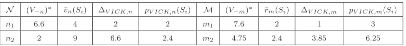
N (V−n)∗ ¯vn(Si) ∆V ICK,n pV ICK,n(Si) M (V−m)∗ r¯m(Si) ∆V ICK,m pV ICK,m(Si)
n1 6.6 4 2 2 m1 7.6 2 1 3
n2 2 9 6.6 2.4 m2 4.75 2.4 3.85 6.25
Table 4: Vickrey discounts and prices.
w∈ W is a participant that is part of the allocation. LetV∗ be the maximized value of the winner
determination problem and (V−w)∗ be the maximized value without the participant w. Thus, the
Vickrey discount for a participantwcan be calculated by ∆V ICK,w=V∗−(V−w)∗. With regards to
the Vickrey discount ∆V ICK,w, the pricepV ICK,n(Si) for a bundleSiand a buyerncan be calculated
by
pV ICK,n(Si) =vn(Si)sn(Si)−∆V ICK,n, (19)
and the pricepV ICK,m(Si) for a bundleSi and a sellermby pV ICK,m(Si) =rm(Si) X n∈N X t∈T ym,n,t(Si) + ∆V ICK,m α . (20)
As sellers submit OR concatenated bids, they can participate in the allocation with multiple bundles. Because the Vickrey discount refers to the seller’s overall impact, the discount has to be portioned among all of the seller’s successful bids. Thus the discount is divided byα, whereαis the number of bundles with which a sellermis participating in the allocation.
Applying the VCG pricing scheme to the example presented above (V∗ = 8.6) results in the
prices pV ICK,w(Si) and the discounts ∆V ICK,w shown in table 4 with ¯vn(Si) = vn(Si)sn(Si) and
¯
rm(Si) =
P
t∈T,n∈Nym,n,t(Si)rm(Si).
As stated by the Myerson-Satterthwaite impossibility theorem, a VCG mechanism is efficient and individually rational but non budget balanced in an exchange. Aggregating the net payments of the example leads to a negative value with 2 + 2.4−(3 + 6.25) =−4.85. In this case, the auctioneer has to subsidize the exchange. Naturally, such a situation cannot be sustained for a long period of time, making the VCG mechanism unfeasible.
Relaxing the requirement of having an efficient allocation opens up the possibility for a second-best mechanism that is budget balanced. These ideas gave rise to the development of ak-pricing scheme which is presented in the next section.
4.3.2 K-Pricing
The underlying idea of the k-pricing scheme is to determine prices for a buyer and a seller on the basis of the difference between their bids (Sattherthwaite and Williams, 1993). For instance, suppose that a buyer wants to purchase a computation service for $5 and a seller wants to sell a computation service for at least $4. The difference between these bids isπ = $1, where π is the surplus of this transaction that can be distributed among the participants.
For a single commodity exchange, thek-pricing scheme can be formalized as follows: letvn(Si) =a
is assumed thata≥b, i.e. the buyer has a valuation for the commodity which is at least as high as the seller’s reservation price. Otherwise no trade would occur. The price for a buyernand a sellermcan be calculated byp(Si) =ka+ (1−k)bwith 0≤k≤1. In regard to the above-mentioned bids for the
computation serviceg1, the resulting price for both participants isp(g1) = 0.5∗9 + (1−0.5)∗2.4 = 5.7 fork= 0.5.
In the following, it is assumed that the number of buyers equals the number of sellers. Therefore,
kis set tok= 0.5 since it favors neither the buyers’ side nor the sellers’ side.
The k-pricing schema can also be applied to a multi-attribute combinatorial exchange: in each time slott in which a bundleSi is allocated from one or more sellers, the surplus generated by this
allocation is distributed among a buyer and the sellers. Suppose a buyern receives a computation serviceS1 ={g1} with 1000 MIPS in time slot 4 and values this slot with vn(S1) = 5. The buyer
obtains the computation service S1 = {g1} by a co-allocation from seller m1 (400 MIPS) with a reservation price ofrm1(S1) = 1 and from sellerm2 (600 MIPS) withrm2(S1) = 2. The distributable
surplus of this allocation isπn,4(S1) = 5−(1 + 2) = 2. Buyern getsk∗πn,4(S1) of this surplus, i.e.
the price buyernhas to pay for this slot is pk,n,4(Si) = v(S1)−kπn,4(S1). Furthermore, the sellers
have to divide the other part of this surplus, i.e. (1−k)πn,4(S1). This will be done by considering
each proportion a seller’s bid has on the surplus. In the example, this proportionom,n,t(Si) for seller m1 isom1,n,4(S1) = 13 and for sellerm2 isom2,n,4(S1) = 23. The price a seller mreceives for a single
slot 4 is consequently calculated as
pk,n,4(Si) =rm(S1) + (1−k)πn,4(S1)om,n,4(S1).
Expanding this scheme to a set of time slots results in the following formalization: letπn,t(Si) be the
surplus for a bundleSi of a buyernwith all corresponding sellers for a time slott: πn,t(Si) =zn,t(Si)vn(Si)− X m∈M X Sl∈S ym,n,t(Sl)rm(Sl) (21)
For the entire job (i.e. all time slots), the price for a buyernis calculated as
pk,n(Si) =xn(Si)vn(Si)sn(Si)−k
X
t∈T
πn,t(Si). (22)
This means that the difference between the valuation for all slots (vn(Si)sn(Si)) of the bundleSi and
thek-th proportion of the sum over all time slots of the corresponding surpluses is determined. The price of a seller m is calculated in a similar way: First of all, the proportionom,n,t(Si) of a
sellermallocating a bundleSi to the buyernin time slott is given by om,n,t(Si) =P ym,n,t(Si)rm(Si)
m∈M P
Sl∈Sym,n,t(Sl)rm(Sl)
. (23)
Having computedπn,t(Si) andom,n,t(Si), the price a seller receives for a bundleSi is calculated as: pk,m(Si) = X n∈N X t∈T ym,n,t(Si)rm(Si) + (1−k) X n∈N X Sl∈S X t∈T om,n,t(Sl)πn,t(Sl). (24)
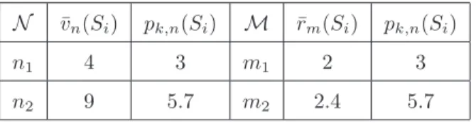
Applying this pricing scheme to the example presented above results in the prices given table 5 with ¯
vn(Si) =vn(Si)sn(Si) and ¯rm(Si) =
X
t∈T,n∈N
In this case, the exchange does not have to subsidize the participants since it fulfills the budget balance property in a way that no payments towards the mechanism are necessary. Hence, thek-pricing schema qualifies as a candidate pricing schema for the Grid. Since the Myerson-Satterthwaite impossibility theorem is strict, the implications of the pricing schema on the allocation need to be investigated.
N v¯n(Si) pk,n(Si) M r¯m(Si) pk,n(Si)
n1 4 3 m1 2 3
n2 9 5.7 m2 2.4 5.7
Table 5: Prices usingk-Pricing withk= 0.5.
5
Evaluation
The presented auction formats are evaluated by means of a stochastic simulation. The winner deter-mination problem is solved using the optimization engine CPLEX 9.1.6 The evaluation assesses the
impact of the auction schemas on the outcome requirements defined in section 2.
5.1
Data Basis
As a data basis, a random bid stream including Decay distributed bundles is generated. The decay function has been recommended by Sandholm (2002) because it creates hard instances of the allocation problem. At the beginning, a bundle consists of one random resource. Afterwards, new resources are added randomly with a probability of α = 0.75. This procedure is iterated until resources are no longer added or the bundle already includes the same resource. The effects that can be obtained by the Decay distribution will be amplified. Hence, the Decay function is used to create a benchmark for upper bounds of the effects.
As an order, buyers and sellers submit a set of bids on 10 different bundles, where a bundle is Decay-distributed from 5 possible resources. Each resource has two different attributes drawn from a uniform distribution in line with most of the quality characteristics of computer resources described by Kee et al. (2004). The time attributes are each uniformly distributed where the earliest time slot has a range of [1..3], the latest time slot is in [4..6], and the number of slots lies in [1..3]. Forty percent of the buyers’ bids have co-allocation restrictions. Sixty percent of the resources contained in these bundles have uniform distributed restrictions on the maximum number of co-allocations. The number of resources which have to be allocated from the same machine (coupling) is also drawn from an uniform distribution.
The corresponding valuations and reservation prices for a bundle are drawn from the same normal distribution, whereas the number of resources in a bundle and the quality characteristics affect the mean and variance of the distribution. This means the probability is greater that a buyer has a higher valuation for a storage service with 200 GB than for a storage service with 10 GB of space. In any
problem instance, new orders for buyers and sellers are randomly generated. Subsequently, demand and supply are matched against each other, determining the winning allocation and corresponding prices.
In total, 120 different problem instances are generated, where a problem consists of 10 or 20 participants. The proportion of buyers and sellers is equally selected out of{10/10, 8/12, 12/8, 5/5, 1/4, 4/1}. In each instance, the buyers and sellers each submit one single bid.
5.2
Truthful Bidders
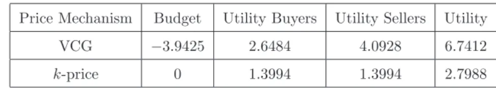
In the first treatment, it is assumed that bidders are truthful. The average results of the treatment regarding the budget balance and participant utilities are shown in table 6.
Price Mechanism Budget Utility Buyers Utility Sellers Utility
VCG −3.9425 2.6484 4.0928 6.7412
k-price 0 1.3994 1.3994 2.7988
Table 6: Average Utility and Budget using Decay distributed bids.
As the Myerson-Satterthwaite theorem suggests, the budget using a VCG auction is always neg-ative. The mechanism requires subsidization from outside the system. Note that these subsidies amount to half the total utility. Obviously, incentive compatibility is extremely expensive, as these subsidizations are required to motivate the buyers and sellers to truthfully report their valuations and reservation prices.
By applying a k-price auction, the budget deficit can be converted into a mechanism, which is independent from outside subsidies. Regarding its formal construction, thek-price auction is budget balanced; however, the average total utility shrinks by the amount of the budget deficit (including a small approximation increment). The share between buyers’ and sellers’ surplus remains unchanged. In thek-pricing schema, however, the utilities of the buyers and sellers are significantly smaller than in the VCG auction and denote a measure for the incentive compatibility loss.
As table 6 shows, the sellers’ utilities in a VCG auction are higher than those of the buyers. Regarding the data basis, sellers expect to offer more available time slots than buyers request. Buyers submit bids on a number of time slotssn(Si) between a time rangeen(Si) and ln(Si). The number
of requested slots is less than the number of allocatable slots, i.e. sn(Si)≤ln(Si)−en(Si). A seller,
however, offers a service for the entire time range. As the time ranges of the buyers and sellers are drawn from the same distribution, the number of tradeable slots a seller offers is greater than the buyer’s requested slots. The greater the number of tradeable slots, the higher the impact of the bid in the VCG mechanism. As such, the sellers’ average discounts are higher than those of the buyers; therefore the sellers have a higher average utility than the buyers.
Because the simulation assumes truthful bidding, this rather naive analysis is only accurate for the VCG mechanism. If the pricing rule is changed – for example from the VCG mechanism to the
compatible.
5.3
Manipulating Bidders
In a second treatment, it is assumed that buyers and sellers using thek-pricing schema misrepresent their true valuation or reservation price respectively. Only simple misrepresentations byβ% are con-sidered, whereλ% of the buyers and sellers reduce or increase their reported values by β%. Instead of observing only symmetric Nash-equilibria as in the analysis by Parkes et al. (2001), where buyers and sellers either misrepresent their valuation or reservation price by 0 or byβ%, the ratio of misrep-resenting buyers and sellers to the total number of participants is also varied. A ratio ofβ = 50%, for instance, denotes that 50% of the buyers and sellers misrepresent their valuations and reservation prices byλ%, while the other 50% report truthfully.
By exploring the joint strategy space (i.e. varying the share of misrepresentative and truthful participants as well as the percentage of misrepresentation) the average efficiency loss for thek-pricing schema can be analyzed: Let ¯n ∈ N¯ be the buyers and ¯m∈ M¯ be the sellers who are part of the allocation in a truthful bidding scenario, i.e. λ=β = 0. Furthermore, let ˆn∈Nˆ be the buyers and
ˆ
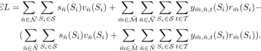
m∈Mˆ be the sellers of the allocation having manipulating bidders (λ≥0, β≥0). Subsequently, the efficiency lossELcan be calculated as the difference between the true preferences of the participants who are part of the allocation in both the truthful and manipulating scenarios:
EL=X ¯ n∈N¯ X Si∈S s¯n(Si)v¯n(Si) + X ¯ m∈M¯ X ¯ n∈N¯ X Si∈S X t∈T ym,¯ n,t¯ (Si)rm¯(Si)− (X ˆ n∈Nˆ X Si∈S sˆn(Si)vˆn(Si) + X ˆ m∈Mˆ X ˆ n∈Nˆ X Si∈S X t∈T ym,ˆ ˆn,t(Si)rmˆ(Si)).
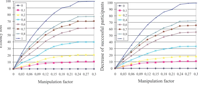
Figure 1 shows the percentage efficiency loss and the percentage decrease of the number of successful bidders with a varying number of manipulating participants as a function of the manipulation factor. For instance, if β = 40% of the participants manipulate their valuations and reservation prices by
λ= 6%, the resulting efficiency loss is 15%. It is apparent that the efficiency loss is higher when more participants use manipulation and thereby increase the manipulation factor. With a manipulation factor greater than λ = 25%, the efficiency curves stagnate. This stagnation results from the fact that either non-manipulating bidders are the only participants of the allocation (in case ofβ <100%) or no one is allocated further (in case of β = 100%). The valuation and reservation prices with a manipulation factorλ >25% are so low – respectively so high – that no bid from the manipulating participants is allocated. This means that no manipulated offer for a bundle can be matched with any manipulated request. This effect is supported by the percentage decrease of the number of successful bidders by manipulating participants. For instance, ifβ = 20% of the participants manipulate their bids byλ= 21%, the number of allocated bids is 17% smaller than in the non-manipulating scenario. Furthermore, if all participants are manipulating byλ= 30%, the size decreases by 100%, i.e. the set of allocated participants is empty. The curves recurrently stagnate with a manipulation factor greater thanλ= 25%.
0 10 20 30 40 50 60 70 80 90 100 0 0,03 0,06 0,09 0,12 0,15 0,18 0,21 0,24 0,27 0,3 Manipulation factor
D
ec
re
as
e
o
f
su
cc
es
sf
u
l
p
ar
ti
ci
p
an
ts
0 0,1 0,2 0,4 0,6 0,7 0,8 1 0 10 20 30 40 50 60 70 80 90 100 0 0,03 0,06 0,09 0,12 0,15 0,18 0,21 0,24 0,27 0,3 Manipulation factor E ff ie nc y lo ss 0 0,1 0,2 0,4 0,6 0,7 0,8 1Figure 1: Efficiency loss (left) and decrease of the number of successful bidders (right) by manipulating participants.
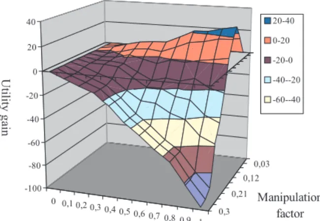
This gives information on whether or not the total utility of participants can be improved through manipulation. The utility which participants can gain by manipulation only depends on the prices they have to pay and is thus calculated as
U G= X ˆ n∈Nˆ X Si∈S ˆ pˆn(Si) + X ˆ m∈Mˆ X Si∈S ˆ pmˆ(Si)−( X ¯ n∈N¯ X Si∈S p¯n(Si) + X ¯ m∈M¯ X Si∈S pm¯(Si)),
where ˆNand ˆM are the sets of buyers and sellers who are part of the allocation with manipulating par-ticipants and ˆpˆn(Si) and ˆpˆm(Si) are the corresponding prices. Sets ¯N and ¯Mdenote the participants
of the allocation in the non-manipulated scenario withp¯n(Si) andpm¯(Si) as their prices.
The percentage utility gain of manipulating participants in the k-price auction is shown in fig-ure 2. The total utility of the participants can be increased by manipulation; at the highest point where all participants manipulate by λ = 6%, the utility gain is more than 26% compared to the non-manipulating scenario. Moreover, small manipulation factors between λ= 1% and λ= 9% al-ways result in a positive utility gain. However, participants have a negative utility gain when the manipulation factor is greater than λ = 13%. In the worst scenario, the utility loss is 100% if all participants manipulate byλ= 30%.
In summary, the simulation has shown it reasonable to believe that participants will not strongly deviate from their truth valuations and reservation prices. Although participants’ average utility gain can be improved through manipulation, the participants increasingly risk not being executed in the auction (cf. figure 1). This risk actually increases the more participants use manipulation. The simulation result suggests that the k-pricing schema has accurate incentive properties resulting in fairly mild allocative efficiency losses. As such, the pricing schema is a practical alternative to the VCG mechanism and is highly relevant for an application in the Grid.
0 0,1 0,2 0,30,4 0,5 0,6 0,7 0,8 0,9 1 0,3 0,21 0,12 0,03 -100 -80 -60 -40 -20 0 20 40 U til ity g ai n Participants manipulating Manipulation factor 20-40 0-20 -20-0 -40--20 -60--40 -80--60 -100--80
Figure 2: Utility gain usingk-pricing.
5.4
Computational Tractability
As denoted in section 2, a computational tractable outcome determination is required. However, the multi-attribute combinatorial winner determination problem (MWDP) isN P-complete: consider the special case of the MWDP with multiple buyers, one seller, no quality attributes, one time slot, and no coupling and maximal divisibility restrictions. In this case, the problem is equivalent to the combinatorial allocation problem (CAP) formulated by Rothkopf et al. (1998). CAP is equivalent to the set-packing problem (SPP) on hypergraphs (Rothkopf et al., 1998) which is known to be N P -complete (Karp, 1972). Since CAP can be reduced to the MWDP, the MWDP is alsoN P-complete. Due to the N P-completeness of the winner determination problem, the auction schema is com-putationally intractable in large-scaled scenarios. For settings with a limited number of participants, however, the auction schema seems practicable. Ideally, an upper boundary of participants can be defined for which the problem is still computationally tractable within a meaningful timeframe. In the context of trading services, a meaningful timeframe is consistent with the maximum time limit that an allocation process may last. Experiences suggest that an allocation process that is shorter than 4 minutes is adequate.
Preliminary studies with the auction schema confirmed that solving the winner determination problem can become computationally intractable, even in settings with less than 100 participants. This implies that exact solutions of the winner determination problem may require too much computation time and cannot be directly applied for the Grid market. To remedy this obstacle, we have to rely on approximations. A common way is to employ algorithms that compute solutions of the winner determination problem within a threshold r away from optimality, say 2%. Such deviations from optimal solutions are often conceived to be tolerable. However, in some cases even finding solutions within the specified threshold of 2% becomes impossible within a meaningful timeframe. In those cases the approximations need to have a termination condition that forces the algorithm to return the best solution found within a predefined time range. Combinatorial auction experiments have shown that these so-calledanytimealgorithms perform fairly well. For instance, Andersson et al. (2000) and
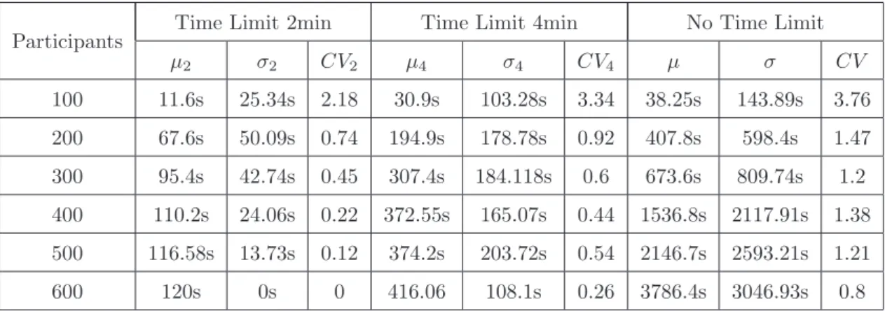
Participants Time Limit 2min Time Limit 4min No Time Limit µ2 σ2 CV2 µ4 σ4 CV4 µ σ CV 100 11.6s 25.34s 2.18 30.9s 103.28s 3.34 38.25s 143.89s 3.76 200 67.6s 50.09s 0.74 194.9s 178.78s 0.92 407.8s 598.4s 1.47 300 95.4s 42.74s 0.45 307.4s 184.118s 0.6 673.6s 809.74s 1.2 400 110.2s 24.06s 0.22 372.55s 165.07s 0.44 1536.8s 2117.91s 1.38 500 116.58s 13.73s 0.12 374.2s 203.72s 0.54 2146.7s 2593.21s 1.21 600 120s 0s 0 416.06 108.1s 0.26 3786.4s 3046.93s 0.8
Table 7: CPU time required to solve the problem.
Sandholm et al. (2005) report that feasible and approximate solutions can be determined in a fraction of time that would be required to find and prove an optimal solution.
The applied standard solver CPLEX provides these functionalities. For our computational tractabil-ity analysis, we perform a series of simulations with anytime approximations for computing the solu-tions. The 4 minutes introduced above will serve as maximum timeframe. To compare the results, we also employ a simulation setting with a more optimistic limit of 2 minutes. As the anytime al-gorithms diverges from the theoretical optimum, we need a measure that captures the welfare loss imputed to the approximation. Nevertheless, computing the theoretical optimum may take very long, so that we use benchmark solution that lies within a 2% gap from the optimum. If CPLEX cannot find any feasible solution within the specified timeframe, the problem instance is rated as intractable. For instance, if no feasible solution is found within 2 minutes, the problem is measured as an empty allocation with welfare of 0 and runtime of 2 minutes. This way, we include those hard instances in our analysis.
In order to perform the simulation, nearly the same random order flow is used as described above. However, the time attributes are widened in order to generate harder and more realistic settings. The earliest time slots are within a range of [1..5], the latest time slots within [6..10], and the number of slots within a range of [1..5]. In the simulation, the proportions of buyers and sellers are equal and the number of participants is varied. In total, 20 treatments are computed and the results are averaged.
Table 7 summarizes the runtime results of the simulations with 2 minutes time limit, 4 minutes time limit, and benchmark solution with no time limit.7 The table shows the meanµ, the standard
deviationσ, and the coefficient of variationCV =σ/µof the CPU times required to solve the winner determination problems. For example, with 200 participants the average runtime with 2 minutes time limit isµ2= 67.6 seconds, with 4 minutes limitµ4= 194.9 seconds, and without a time limitµ= 407.8 seconds. Note that the differences in the runtime of settings with equal number of participants are caused by the underlying time limits. For 200 participants, several instances require more than 2 minutes, some even more than 4 minutes to find a solution within the specified gap. As CPLEX terminates after the predefined timeframe, the average runtime in the 2 minutes setting is less than
7The analysis was performed on a Pentium XEON with 3.2GHz and 2GB ram using CPLEX 9.1 with a MIP gap of
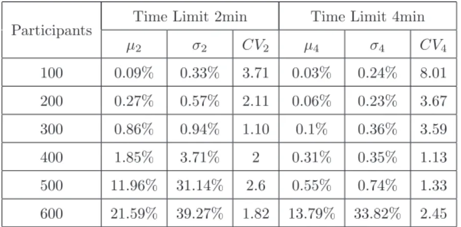
Participants Time Limit 2min Time Limit 4min µ2 σ2 CV2 µ4 σ4 CV4 100 0.09% 0.33% 3.71 0.03% 0.24% 8.01 200 0.27% 0.57% 2.11 0.06% 0.23% 3.67 300 0.86% 0.94% 1.10 0.1% 0.36% 3.59 400 1.85% 3.71% 2 0.31% 0.35% 1.13 500 11.96% 31.14% 2.6 0.55% 0.74% 1.33 600 21.59% 39.27% 1.82 13.79% 33.82% 2.45
Table 8: Percentage Welfare Loss
the runtime required for finding the benchmark solution.
With an increasing number of participants, CPLEX’s average execution time grows rapidly. This is most obvious in the benchmark settings with no time limit. For 500 participants, CPLEX requires nearly 2 hours to find a solution for some instances. In some settings with 600 participants, CPLEX even fails in finding a benchmark solution within 2 hours. In those cases, the simulation is stopped and the obtained results are neglected. More precisely, in our analysis this status occurred in 8 out of 20 instances. As these cases do not produce benchmark solutions, the obtained results with 600 participants may only have marginal significance.
Overall, the runtime analysis shows that the winner determination problem is computationally intractable without the introduction of time limits. Apparently, delimiting the approximation produces solutions in a meaningful time, i.e. less than 4 minutes.
In settings with limited time, however, the quality of the (suboptimal) solutions and accordingly its impact on the welfare changes. In the following the welfare effect due to the approximations is studied in detail. For this, we define a welfare loss higher than 5% as unacceptable for our settings, as we already have approximate solutions via the applied 2% gap.
Table 8 summarizes the welfare loss of the time limited scenarios compared to the benchmark solution. For instance, for 300 participants the average welfare loss in the 2 minutes setting isµ2 = 0.86% and in the 4 minutes limit µ4= 0.1%. With an increasing number of participants, the welfare loss becomes higher. On the one hand, this is reasoned by the fact that the problem instances become harder to solve within the given time frame. On the other hand, feasible solutions cannot always be found in time which results in a welfare loss for these infeasible instances of 100%. This explains the big increase of the welfare loss from 400 to 500 participants in the 2 minutes settings – respectively, from 500 to 600 participants in the 4 minutes settings. Regarding the simulations with a limit of 2 minutes, the welfare loss exceeds our 5% threshold for more than 400 participants. With a 4 minutes limit, this threshold is exceeded in settings with more than 500 participants.
The analysis of the welfare loss shows, that the anytime algorithm achieves fairly efficient results: With a 2 minutes time limit, the welfare loss is acceptable for scenarios with up to 400 participants. For settings with up to 500 participants, a time limit of 4 minutes entails reasonable results. However, the applied time limits become useless for settings with more than 500 participants. For such cases,
the use of other approximations has to be considered.
To anchor the problem to real Grid applications and to provide insights to practitioners, we stud-ied the characteristics of PlanetLab8 and compared them to our computational results. Essentially,
PlanetLab is a testbed for networking and distributed computing among several scientific institutes worldwide. The network is state-of-the-art and currently the largest infrastructure for sharing compu-tational Grid services. The user information was obtained using the data provided by the All-Pairs-Pings project9. We collected and analyzed the available data from November 2005 until March 2006.
As a result, PlanetLab has currently µ = 170.89 active machines on average which can be used to perform computational jobs (with a standard deviation of σ = 21.33). The coefficient of variation (CV) for the valuesCV =σ/µ= 0.12 shows that the variability in reference to the size of the mean is low. Thus, the determined average constitutes to be a stable value.
Transferring the PlanetLab characteristics to the proposed auction schema implies 170 sellers on average. Assuming an equal number of buyers and sellers, the average number of participants in the PlanetLab scenario is 340. With respect to the above presented results, the application of a 2 minutes time limit is sufficient to fulfill PlanetLab resource bids in a meaningful time. In cases the boundary raises up to 500 participants, a time limit of 4 minutes is preferable. For larger settings, however, alternative approaches have to be evaluated.
6
Conclusion
The paper at hand proposes the derivation of a multi-attribute combinatorial exchange for allocating and scheduling services in the Grid. In contrast to other approaches, the proposed mechanism accounts for the variety of services by incorporating time and quality as well as coupling constraints. The mechanism provides buyers and sellers with a rich bidding language, allowing for the formulation of bundles expressing either substitutabilities or complementarities. The winner determination problem maximizes the social welfare of this combinatorial allocation problem. The winner determination scheme alone, however, is insufficient to guarantee an efficient allocation of the services. The pricing scheme must be constructed in a way that motivates buyers and sellers to reveal their true valuations and reservation prices. This is problematic in the case of combinatorial exchanges, since the only efficient pricing schedule, the VCG mechanism, is not budget-balanced and must be subsidized from outside the mechanism.
This paper develops a new pricing family for a combinatorial exchange, namely thek-pricing rule. In essence, thek-pricing rule determines the price such that the resulting surpluses to the buyers and sellers divide the entire surplus being accrued by the trade according to the rationk. The k-pricing rule is budget-balanced but cannot retain the efficiency property of the VCG payments.
As the simulation illustrates, the k-pricing rule does not rigorously punish inaccurate valuation and reserve price reporting. Buyers and sellers sometimes increase their individual utility by cheating.
8Seehttp://www.planet-lab.org/for details.
9Every 15 minutes, all registered nodes are contacted to check their availability status. Seehttp://ping.ececs.uc. edu/ping/for details.
This possibility, however, is only limited to mild misreporting and a small number of strategic buyers and sellers. If the number of misreporting participants increases, the risk of not being executed in the auction rises dramatically. As a result, the k-pricing schema is a practical alternative to the VCG mechanism and highly relevant for an application in the Grid. The runtime analysis shows that the auction schema is computationally very demanding. However, the use of approximated solutions achieves adequate runtime results and fairly mild welfare losses for up to 500 participants. Comparing these results with an existing Grid testbed evinces the practical applicability of the proposed auction. This paper is a step towards understanding the effect and strength of different multi-attribute combinatorial exchange mechanisms on efficiency. Contributions include detailing a realistic market definition for Grid services, deriving the domain-specific requirements from the Grid, defining a winner determination scheme that meets these requirements, exploring adequate pricing schemes that contain the right incentives, and evaluating the market mechanism by means of a simulation.
Future research needs to consider alternative heuristics that simplify the winner determination problem. Nature-inspired algorithms such as genetic algorithms may be adequate for an application in the service market. A further step towards a functioning Open Grid Market would be to confront the mechanism with real data in a pilot run.
Acknowledgements
This work has partially been funded by EU IST progamme under grant 003769 “CATNETS”. The authors are grateful to the anonymous reviewers for the constructive comments and suggestions that significantly improved the paper.
References
Andersson, A., Tenhunen, M., Ygge, F., 2000. Integer Programming for Combinatorial Auction Win-ner Determination. In: ICMAS ’00: Proceedings of the Fourth International Conference on Multi-Agent Systems. IEEE Computer Society, Washington, DC, USA, pp. 39–46.
Bapna, R., Das, S., Garfinkel, R., Stallaert, J., 2005. A Market Design for Grid Computing. Tech. rep., Department of Operations and Information Management, University of Connecticut.
Buyya, R., Abramson, D., Giddy, J., Stockinger, H., 2002. Economic Models for Resource Management and Scheduling in Grid Computing. The Journal of Concurrency and Computation: Practice and Experience 14 (13-15), 1507–1542.
Clarke, E., 1971. Multipart pricing of Public Goods. Public Choice 2, 19–33.
Eymann, T., Reinicke, M., Ardaiz, O., Artigas, P., de Cerio, L. D., Freitag, F., Messeguer, R., L. Navarro, D. R., 2003. Decentralized vs. Centralized Economic Coordination of Resource Alloca-tion in Grids. In: Proceedings of the 1st European Across Grids Conference.
Foster, I., Kesselman, C., 2004. The Grid 2 - Blueprint for a New Computing Infrastructure. Vol. 2. Elsevier.
Foster, I., Kesselman, C., Nick, J., Tuecke, S., 2002. Grid Services for Distributed System Integration. IEEE Computer 35 (6), 37–46.
Green, J., Laffont, J.-J., 1977. Characterization of Satisfactory Mechanisms for the Revelation of Preferences for Public Goods. Econometrica 45 (2), 427–438.
Groves, T., 1973. Incentives in teams. Econometrica 41, 617–631.
Jackson, M. O., 2002. Mechanism Theory. In: Encyclopedia of Life Support Systems. Eolss Publishers, Oxford ,UK.
Karp, R. M., 1972. Reducibility among Combinatorial Problems. In: Miller, R. E., Thatcher, J. W. (Eds.), Complexity of Computer Computations. Plenum Press, pp. 85–103.
Kee, Y.-S., Casanova, H., Chien, A., 2004. Realistic Modeling and Synthesis of Resources for Compu-tational Grids. In: ACM Conference on High Performance Computing and Networking (SC2004). ACM Press.
Lai, K., 2005. Markets are Dead, Long Live Markets. Tech. Rep. 0502027, HP Labs.
Ludwig, H., Dan, A., Kearney, B., 2004. Cremona: An Architecture and Library for Creation and Monitoring of WS-Agreements. In: Proceedings of the 2nd International Conference on Service Oriented Computing (ICSOC 2004). pp. 65–74.
Milgrom, P., 2004. Putting Auction Theory to Work. Cambridge University Press.
Myerson, R. B., Satterthwaite, M. A., 1983. Efficient Mechanisms for bilateral Trading. Journal of Economic Theory 28, 265–281.
Neumann, D., 2004. Market Engineering – A Structured De