DigitalCommons@University of Nebraska - Lincoln
DigitalCommons@University of Nebraska - Lincoln
Publications, Agencies and Staff of the U.S.
Department of Commerce
U.S. Department of Commerce
2007
Space–time zero-inflated count models of Harbor seals
Space–time zero-inflated count models of Harbor seals
Jay M. Ver Hoef
National Marine Mammal Laboratory, Alaska Fisheries Science Center, NOAA Fisheries
John K. Jansen
Follow this and additional works at: https://digitalcommons.unl.edu/usdeptcommercepub Part of the Environmental Sciences Commons
Ver Hoef, Jay M. and Jansen, John K., "Space–time zero-inflated count models of Harbor seals" (2007). Publications, Agencies and Staff of the U.S. Department of Commerce. 182.
https://digitalcommons.unl.edu/usdeptcommercepub/182
This Article is brought to you for free and open access by the U.S. Department of Commerce at
Published online 7 August 2007 in Wiley InterScience (www.interscience.wiley.com) DOI: 10.1002/env.873
Space–time zero-inflated count models of Harbor seals
‡Jay M. Ver Hoef
∗,†and John K. Jansen
National Marine Mammal Laboratory, Alaska Fisheries Science Center, NOAA Fisheries, 7600 Sand Point Way NE, Building 4, Seattle WA 98115-6349, U.S.A.
SUMMARY
Environmental data are spatial, temporal, and often come with many zeros. In this paper, we included space–time random effects in zero-inflated Poisson (ZIP) and ‘hurdle’ models to investigate haulout patterns of harbor seals on glacial ice. The data consisted of counts, for 18 dates on a lattice grid of samples, of harbor seals hauled out on glacial ice in Disenchantment Bay, near Yakutat, Alaska. A hurdle model is similar to a ZIP model except it does not mix zeros from the binary and count processes. Both models can be used for zero-inflated data, and we compared space–time ZIP and hurdle models in a Bayesian hierarchical model. Space–time ZIP and hurdle models were constructed by using spatial conditional autoregressive (CAR) models and temporal first-order autoregressive (AR(1)) models as random effects in ZIP and hurdle regression models. We created maps of smoothed predictions for harbor seal counts based on ice density, other covariates, and spatio-temporal random effects. For both models predictions around the edges appeared to be positively biased. The linex loss function is an asymmetric loss function that penalizes overprediction more than underprediction, and we used it to correct for prediction bias to get the best map for space–time ZIP and hurdle models. Published in 2007 by John Wiley & Sons, Ltd.
key words: spatial statistics; time series; Poisson; Bernoulli; hurdle model; linex loss function
1. INTRODUCTION
Environmental data are spatial, temporal, and often come with many zeros. Statisticians are developing models of increasing complexity to handle these data. Time series (e.g., Brockwell and Davis, 1991), spatial statistics (e.g., Cressie, 1993), and zero-inflated Poisson (ZIP) regression (e.g., Lambert, 1992; Welshet al., 1996) are all becoming well-developed subjects. There are increasing numbers of examples where models combine these subjects, such as space–time models for Gaussian data (Wikleet al., 1998), temporal ZIP models (Dobbie and Welsh, 2001; Leeet al., 2006), and spatial ZIP models (Agarwal
et al., 2002; Rathbun and Fei, 2006). Wikle and Anderson (2003) developed a space–time ZIP model for tornado counts that is very similar to our development. A hurdle model (Cragg, 1971) is similar to a ZIP model except it does not mix zeros from the binary and count processes. In this paper, we use the standard formulation of ZIP and hurdle models and develop Bayesian hierarchical models with space–time errors to investigate haul-out patterns of harbor seals on glacial ice.
∗Correspondence to: J. M. Ver Hoef, National Marine Mammal Laboratory, Alaska Fisheries Science Center, NOAA Fisheries,
7600 Sand Point Way NE, Building 4, Seattle, WA 98115-6349, U.S.A.
†E-mail: jay.verhoef@noaa.gov
‡This article is a U.S. Government work and is in the public domain in the U.S.A.
We have two main objectives with this paper. First, we compare the space–time ZIP and hurdle models and how they differ in terms of estimated parameters, predictions, and precision. Secondly, we use a model diagnostic for these two space–time zero-inflated models, and we note that there are bias concerns when using either the mean or median as a summary of posterior predictions for creating smoothed maps. This leads us to investigate the linex loss function (Varian, 1975), which corrects for the bias.
2. DATA
The data consist of counts of harbor seals hauled out on glacial ice in Disenchantment Bay, near Yakutat, Alaska. Aerial surveys were conducted twice a week, weather permitting, starting 27 May and ending on 4 August in 2002, after the completion of pup rearing. These surveys were timed to facilitate a comparison of seal abundance and distribution between periods of low and high numbers of cruise ship visits to the bay. Surveys were flown between 13:00 and 15:00 h (Alaska Daylight Time) to coincide with the daily peak in numbers of seals hauling out. A single engine aircraft (Cessna 206; Yakutat Coastal Airways Inc., Yakutat, AK) was flown at a target speed of 90–100 knots and altitude of 305 m (1000 ft). From the aircraft, digital video was taken of the entire study area. There are 18 time events (i.e., surveys) that we indexi=1,2, . . . ,18. Sample units were created on a lattice of 400×400 m cells for the entire study area; the spatial locations were on a 19 by 41 grid that we arbitrarily number,j=1,2, . . . , m.
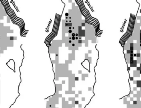
The number of seals was counted in each cell for each date from the digital video. Grid cells that did not have ice had no possibility for seals to haul out, and not all grid cells had ice for each date. Any such grid cells for that date were eliminated. In all there were 2489 records that contained ice over the 18 time periods for the 19 by 41 grid. Data for three dates in May 2002, are shown in Figure 1. The case for
Figure 1. Spatial distribution of harbor seals and ice cover for 3 of 18 dates during summer 2002. The range of seal countsper
grid cell is shown in three levels: small dot (<5 seals), medium dot (5–20 seals), and large dot(>20 seals). Increasing ice cover is represented by three levels: scattered (light gray), intermediate (medium gray), and dense (dark gray)
Figure 2. Histogram of all seal count data showing a high proportion of zeros
zero inflation can be seen from a histogram of all 2489 count values in Figure 2. We also had covariates that varied both spatially and temporally. For each cell and each date, we had: (1) the percentage of the cell covered with ice, in 10 classes at 10% intervals, (2) the closest distance between a ship’s path and the cell, and (3) an activity index that combined the closest approach by a ship and the time that ships spent near a cell. We call these the spatiotemporal covariates. In addition, we had five covariates that varied only temporally (i.e., they applied to all cells for a given date): (1) the presence of a ship on the day of a seal count, (2) number of ships within three days prior to a count, (3) total precipitation in the 6 h prior to a count, (4) maximum wind speed in 6 h prior to a count, and (5) the total number of cells with ice. We call these the temporal covariates. Greater detail on the methods and data can be found in Jansenet al. (2006).
3. MODELS FOR ZERO-INFLATED COUNT DATA
A simple space–time ZIP regression model can be constructed by using spatial conditional autoregressive (CAR) models and temporal first-order autoregressive (AR(1)) models for random effects in a ZIP regression model. A ZIP regression model is given by
Zi,j|Yi,j=
0 ifYi,j=0,
Poi(λi,j) ifYi,j=1. (1)
where Poi(λi,j) is a conditionally independent Poisson random variable with mean functionλi,jandYi,j is an independent Bernoulli random variable with mean functionpi,j;Yi,j∼Bern(pi,j), for theith time
and thejth spatial location. Now we use link functions, as is common for generalized linear models (McCullough and Nelder, 1989) to relate the means of these distributions to a linear mixed model,
log(λi,j)=νi+xi,jβ+i,j,
logit(pi,j)=µi+xi,jα+δi,j, (2) where logit(a)≡log(1−aa),νiandµi are separate means for each time,βandαare 12×1 vectors of regression parameters (for ten ice classes and the distance and activity index), andxi,jare the afore-mentioned spatio-temporal covariates. These covariates, such as per cent ice in a sample unit, change spatially and temporally due to glacial activity, weather and tidal currents. The random errorsi,jand
δi,jare assumed to be spatially autocorrelated for a fixed time eventi. In Equation (2), we assume that each time period has a separate and independent realization of a spatial process fori,jandδi,j. We use a CAR model (see Besag, 1974 and Cressie, 1993, p. 407) for each time period,
δi =Gau(0, σδ2(I−ρδC)−1M)
i =Gau(0, σ2(I−ρC)−1M) (3) where the spatial process for theith time periodδiis independent of the spatial processδi wheni=i, and similarly the spatial processiis independent of the spatial processi wheni=i. Gau(·,·) is a (multivariate) Gaussian (normal) distribution. We defined a neighbor of a sample as any other sample with its centroid within 1 km. We chose this distance because some cells could be isolated, and there is often a checkerboard pattern to cells with ice (Figure 1), and to ensure some smoothing from neighboring values, we wanted cells that were conditionally dependent on some neighbors. The weights inCwere row-standardized (Haining, 1990, p. 82); that is, each row inCcontains all zeros except for columns that indicate a neighbor, and the weights are the reciprocal of the number of neighbors for that sample. The matrixMis a diagonal matrix where the diagonal elements contain the reciprocal of the number of neighbors. Note that we allow the spatial autocorrelation parameters to be constant across time periods. We believe this is reasonable as it represents the seals innate tendency to cluster as groups, and is not likely to change with time.
In a fixed effects model, we would assume thatνi andµi are separate means for each time; here we treat them as separate linear models for temporal covariates, such as the weather on the day of the photograph that affects all spatial locations equally,
νi =ν0+tiη+ξi,
µi =µ0+tiγ+τi,
(4)
wheretiare the temporal covariates. It is here that we allow temporally autocorrelated errors, which are modeled with AR(1) models,
ξi=φξξi−1+σξWξ,i; i >1,
τi=φττi−1+στWτ,i; i >1,
(5)
3.1. A nonmixture model
The ZIP model is important when zeros are a mixture of two distributions; a binary distribution and a count distribution that includes zero. In other words, an observed zero in the ZIP model could be a one from the binary distribution but the count distribution created the observed zero. When considering harbor seal counts on ice, as in our application, the binary distribution is the absence or presence of harbor seals, and the count distribution is the number of seals. If there are detectability issues, this model is appropriate because it expresses the idea that an observed count can be zero even though seals are present; i.e., some seals are undetected. However, in our application, we have good quality video showing a high contrast between the dark seals and the lighter-colored ice on which they are hauled out; seals are thus highly likely to be detected. Hence, we consider models that completely specify and separate the binary distribution from the count distribution, which have been called hurdle models or two-stage models in econometrics (Cragg, 1971; Mullahy, 1986; Heilbron, 1994). Hurdle and ZIP models are reviewed in Ridoutet al. (1998), with a recent comparison of hurdle and ZIP models in Potts and Elith (2006). The hurdle models arise naturally in botany and economics. For example, purchasing patterns of individuals may be modeled where a person decides to purchase items (the binary model is a purchase decision), and then a count model (now defined on positive integers) for the number of items purchased. These models are no longer a mixture, but there is clearly an overabundance of zeros when compared to a simple Poisson distribution, so hurdle models are logically tied to ZIP models and can be compared to them on a purely model-fitting basis. We term our hurdle model as ‘(Poisson + 1)/Binary’ and denote it P1B. For its formulation as a space–time model, we modify Equation (1) to be,
Zi,j|Yi,j=
0 ifYi,j=0,
Poi(λi,j)+1 ifYi,j=1. (6)
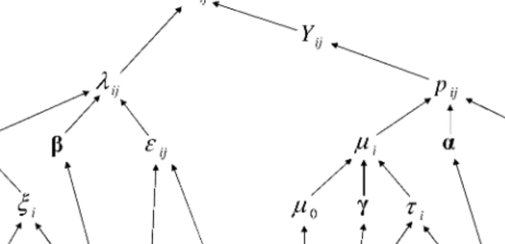
The rest of the model follows exactly as in the ZIP, using Equations (2–5). The dependencies of the model parameters for both ZIP and P1B are shown as a directed graph in Figure 3.
Figure 3. Directed graph of parameter dependencies in ZIP and P1B hierachical model. All prior distributions are denoted by
We note that other distributions could be used in these zero-inflated models. In Equations (1) and (6), we could replace the Poisson distribution with a negative binomial or generalized Poisson (Consul, 1989). Either of these distributions allows for models that are overdispersed relative to a Poisson distribution. With zeros removed, the mean of the rest of the count data is 5.4 after subtracting 1 from all of them. Assuming a Poisson distribution with a mean of 5.4 on these data, the probability of getting a value greater than 20 is 2.8×10⁻⁷, yet it is apparent from Figure 2 that there are many values above 20. On the other hand, the fixed covariate effects and the spatial and temporal random effects can absorb some overdispersion. We tried using a negative binomial, NB(µ, κ), parameterized such that if
Y ∼NB(µ, κ), then E(Y)=µand var(Y)=µ+κµ2. The estimated value ofκwas very near to zero, indicating a linear variance relation to the mean, just like a Poisson, so we do not consider it further. Other distributions could be used in Equation (6), such as a truncated Poisson. Any distribution with support on the positive integers would be mathematically appropriate. We used the ‘Poisson plus one’ because it was easy to implement and has readily interpretable parameters. The main point of the paper is not an exhaustive comparison of all the models, but rather the comparison of a model where zeros are mixed from the Poisson and Bernoulli distributions, versus when there is no mixture.
3.2. Priors
We put diffuse priors on all regression parameters:α,β,γ, andηas defined in Equations (2) and (4). By ‘diffuse,’ we mean as noninformative as we could make them; however, because these parameters are modeled on a log scale, there are computational instabilities if they are allowed to get too large. Hence, we let each regression parameters have a normally distributed prior with a variance of ten. To maintain stationarity, the autoregression parameters for both space (ρδandρ) and time (φτ andφξ) are bounded from−1 to 1 and may have a uniform prior on this range (e.g., Hay and Pettitt, 2001). We did not expect any negative autocorrelation, however, so we used uniform priors from 0 to 1. For the variance parameters of the random effects (σ2δ,σ2,σξ2, andσ2τ), we let the square root be uniformly distributed between 0 and 10; again, to keep the random effects from becoming too large and causing numerical instability. Uniform priors on the square root of variance parameters in hierarchical models has recently been suggested by Gelman (2006), and a simulation study (Lambertet al., 2005) shows that they compare favorably to others and allow the range to be restricted to reasonable values.
3.3. Estimation
Models were fit using Markov Chain Monte Carlo (MCMC) in WinBUGS software§
(Version 1.4, Imperial College and MRC, UK). We used a burn-in of 5000 iterations, and then used 50 000 iterations for estimates and 95% credibility intervals on all parameters and functions of parameters. Because of storage issues (approximately 2500 parameters each forλi,j,pi,j, and their product), we thinned the chain by storing every 50th iteration, resulting in 1000 stored valuesperparameter. The MCMC chains moved freely within their range (they were mixing well), and all parameters passed the test for stationarity using the method of Heidelberger and Welch (1983), as implemented in the CODA package (Bestet al., 1995) in R (R Development Core Team, 2006). During the MCMC sampling, the parameters rarely approached the bounds of the prior distributions as described in the previous section.
Figure 4. Posterior distributions of the autoregressive parameters for the ZIP model
4. RESULTS
4.1. Autoregressive parameters
The posterior distributions of the autoregressive parameters in the AR(1) model and the CAR model, for both the Bernoulli and Poisson parts of the ZIP model, are shown in Figure 4. The posterior distributions of the autoregressive parameters in the AR(1) model and the CAR model, for both the Bernoulli and Poisson parts of the P1B model, are shown in Figure 5. These figures show that there is not a great deal of difference between the models for the autocorrelation parameters. For the P1B model (Figure 5), the spatial autocorrelation parameter for the Poisson distribution appears to be centered around 0.8, whereas the same parameter for the ZIP model is nearer to 0.95 (Figure 4). Also, there appears to be more evidence of positive temporal autocorrelation for the Poisson distribution in the P1B model than the ZIP model.
4.2. Standardized selection coefficients
We obtained the posterior distributions of all regression parameters β, α, η, and γ. Most of them contained zero in the 95% credibility interval. By far the most significant effect was the proportion of ice in the cell. From now on, we consider only this effect. Our conclusions about comparing P1B versus ZIP models for this effect apply equally to all of the others. For a full biological interpretation of all regression effects, see Jansenet al. (2006).
When working with categorical covariates in logistic regression, coefficients are often interpreted on the logit scale, which are the ‘log odds,’ or by exponentiating, which are the ‘odds ratio’ (see Hosmer and Lemeshow, 1989, pp. 40–41). Let us denote ice cover parameters as the first fixed effect with subscript 1:α[1k]for thekth category of ice cover, wherek=1, . . . ,9 (there were no cells with 90–100% ice). For identifiability, suppose thatα[1]1 =0. Then, the odds ratio of seals selecting thekth ice category over the first category is exp(α[1k]). However, this really only facilitates comparing a single category to a reference category for a given model. Here, we will want to compare the coefficients between models. In the resource selection literature, authors often create standardized selection coefficients (e.g., Manly
et al., 2002, p. 51), which, when applied to logistic regression, are odds ratios that sum to one,
˜ α[k] 1 = eα[1k] 9 k=1eα [k] 1 . (7)
Note that these are invariant to the choice of a reference category. That is, if we set ˇα[1k]=α[1k]+Cfor allkand anyC, Equation (7) will remain unchanged. In addition, because the coefficients sum to one, they can be viewed as probabilities. The standard interpretation is that they represent the probability that an animal will select a particular category of a resource, given that each category is equally available. Likewise, for the Poisson part of the model,
˜ β[1k]= eβ[k] 1 9 k=1eβ [k] 1 . (8)
The standardized selection functions can be seen in Figure 6, which suggests that seals tend to prefer ice coverage classes between 5 and 7 (40–70% ice cover). The most interesting comparison of ZIP versus P1B occurs in Figure 6B; note that the 95% credibility intervals are much wider for the ZIP model than for the P1B model. This makes sense because the zeros are mixtures of Poisson and Bernoulli distributions under the ZIP model, so we are less certain about any effect on Bernoulli probabilities. One might also expect slightly narrower credibility intervals for P1B models because we used ‘Poisson(λ)+1.’ Thus, for a fixed count value theλparameter is smaller, and thus the variance is smaller, for the P1B than for the Poisson(λ) from the ZIP model. However, this effect is not readily apparent in Figure 6A.
4.3. Smoothed predictions
For the ZIP model, predictions for each cell at each time may be formed by employing the posterior distribution of the Bernoulli probabilitiespi,j, the expected Poisson countλi,j, and their productλi,jpi,j. For the P1B model we replaceλi,jwith (λi,j+1). The spatial and temporal autocorrelation in the models
Figure 6. Posterior distributions of standardized selection coefficients of ice type for Poisson (A) and Bernoulli (B) parts of the ZIP and P1B models. The ZIP model estimates are shown as dashed lines, and the P1B are shown as solid lines. The vertical lines are the 95 per cent credibility intervals for each estimate for each ice class. The horizontal dotted line is the hypothesis of
equal selection for each type (=1/9)
causes these predictions to rely on neighboring values, so they tend to be ‘smooth,’ especially in relation to the original data. In Figures 7–11 all cells for thei=3 time period that had ice have a predicted value. Obviously, we could do this for any of the 18 time periods. Note that it would be difficult to project into the future without some models for projecting all of the covariates into the future as well. In Figures 7–11, we sized each circle taking the median divided by the interquartile range (75% value minus the 25% value), from the MCMC sample; in that way, values where we have more confidence are larger and more dominant to the eye.
In Figure 7, we show the Bernoulli predictionsp3,jfor all cells. One of the distinctions between ZIP and P1B is in the estimates of the Bernoulli probabilities. An observed zero for the P1B model is a zero for the Bernoulli distribution. However, an observed zero in the ZIP model could be a one from the Bernoulli distribution but the Poisson distribution created the observed zero. Hence, the ZIP model tends to estimate a higherpi,jthan the P1B model, which can be seen from the legends in Figure 7.
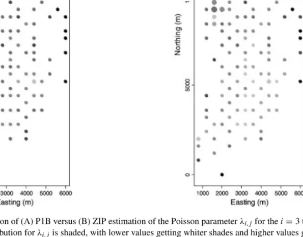
In Figure 8, we show the Poisson predictionsλ3,j for all cells. The count distribution for a P1B begins at one, rather than at zero for the ZIP. Hence, in contrast to the Bernoulli distribution, the count
Figure 7. Comparison of (A) P1B versus (B) ZIP estimation of the Bernoulli parameterpi,jfor thei=3 time period. The mean of the posterior distribution forpi,jis shaded, with lower values getting whiter shades and higher values getting blacker shades.
The size of the circle is inversely proportional to the posterior range scaled by the posterior median
distribution means for the P1B (having a one added to a Poisson random variable) tends to be higher than the mean of the count distribution for the ZIP.
One of the most interesting features in Figure 8 is an edge effect. Notice that the most observed nonzero counts (see Figure 1) occur in the areas where the circles are largest in Figure 8, which is near the upper center. Yet some of the highest predicted values occur along the edges in Figure 8, which cannot be explained by the ice covariate (see Figure 1). We propose the following explanation. All of the modeling is occuring on the log scale. There is greater prediction uncertainty near the edges than near the observed nonzero counts. This is a feature that is often found in prediction methods such as kriging; the farther away you get from the observed data, the higher the prediction variance. We want to make inference on the original scale of the data, so we exponentiate the MCMC values and then average. However, it is well known that ifZ1andZ2are random variables, and E(Z1)=E(Z2) but var(Z1)>var(Z2), then E(eZ1)>E(eZ2). This is clearly causing bias around the edges where there is high prediction variance. We might consider the median instead, as quantiles are unaffected by monotone transformations. Indeed, that corrects the problem seen at the edges of Figure 8. We return to this issue in the next subsection.
Figure 8. Comparison of (A) P1B versus (B) ZIP estimation of the Poisson parameterλi,jfor thei=3 time period. The mean of the posterior distribution forλi,jis shaded, with lower values getting whiter shades and higher values getting blacker shades.
The size of the circle is inversely proportional to the posterior range scaled by the posterior median
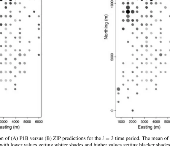
The P1B Bernoulli distribution had a lower mean than the ZIP Bernoulli distribution, but the P1B Poisson distribution had a higher mean than the ZIP Poisson distribution. As a consequence, the smoothed predictions obtained from the posterior means ofλ3,jp3,jcan look quite similar. However, notice the same edge effect in Figure 9 that occurs for the Poisson distribution seen in Figure 8. All in all, these maps are not satisfactory, so we investigate alternatives.
4.4. A model diagnostic and linex loss
Model diagnostics are important in any data analysis. In this section we concentrate on a simple diagnostic for the smoothed prediction maps. Our main concern is with the edge effects described in the previous section. Compare the observed data in Figure 1 for 7 May 2002 to the smoothed predictions in Figure 9B. The predictions in Figure 9B are neither as high as the highest observed values, nor as low as the lowest observed values, which justifies the use of the word ‘smooth.’ However, we might expect that thetotalof the observed counts for 7 May 2002 to be approximately equal to thetotalof the predictions in Figure 9B. One very simple model diagnostic then is to sum the predicted values as in Figure 9, but for each time period. Then, we can sum the observed values for each time period, and compare them.
Figure 9. Comparison of (A) P1B versus (B) ZIP predictions for thei=3 time period. The mean of the posterior distribution forλi,jpi,jis shaded, with lower values getting whiter shades and higher values getting blacker shades. The size of the circle is
inversely proportional to the posterior range scaled by the posterior median
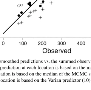
A scatterplot of the sum of the smoothed predicted values versus the sum of the observed values for all 18 time periods is given in Figure 10. Notice that when smoothing by using the mean of the posterior distribution, the summed predictions are greater than the summed observations for all time periods. If we smooth by using the median of the posterior distribution, the summed predictions are less than the summed observations for all time periods. The mean of the posterior is the optimal predictor when using squared-error loss, and the median is the optimal predictor when using absolute deviation loss (see, e.g., Bain and Engelhardt, 1987, pp. 297–298). Because of the skewness of lognormal processes, we decided to use the linex loss function instead.
The linex loss function (Varian, 1975) is an asymmetric loss function given by
L(θ)=eaθ−aθ−1. (9)
The parameteracontrols the amount of asymmetry, with the higher the value ofa, the more asymmetry. This loss function penalizes positive deviations from zero more than negative deviations from zero. The
Figure 10. Scatterplot of the summed smoothed predictions vs. the summed observations for each time period for P1B model. The open circles are the sums when the prediction at each location is based on the mean of the MCMC sample. The crosses are the sums when the prediction at each location is based on the median of the MCMC sample. The solid circles are the sums when
the prediction at each location is based on the Varian predictor (10) from the MCMC sample
optimal predictor for the linex loss function, Equation (9) is given by Zellner (1986); ˆ
θ= −(1/a) log(Eθe−aθ), (10)
and we will call this the Varian predictor. For any parameterθ, we replace the expectationEθe−aθwith an average ofe−aθk, whereθkis thekth sample ofθfrom the MCMC sampler. We applied ˆθto all cell predictions for all dates for various values ofain Equation (10). By trying to match the sum of the smoothed predictions to the sum of the observed values for each date, we determined thata=0.05 to be a reasonable value, as shown in Figure 10.
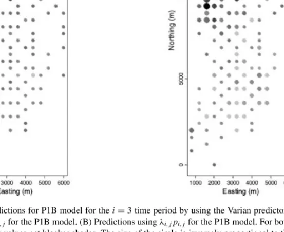
In Figure 11, we show the Poisson predictionsp3,jand the product predictionsp3,j(λ3,j+1) using Equation (10) witha=0.05 for all cells of the P1B model only. The optimal predictions using the linex loss function in Figure 11 has lowered the values around the edges seen in Figure 9, and hence corrected the edge effects. The sum of the smoothed values in Figure 11B is now also close to the sum of the observed values as shown in Figure 10.
5. DISCUSSION AND CONCLUSIONS
Zero-inflated models for count data are appropriate in many situations, and it is important to begin to incorporate space–time dependencies in these models. Such models have been developed for the ZIP regression by Wikle and Anderson (2003). Here, we add the P1B model, which is a simpler approach because there is no mixture of the Bernoulli and Poisson distributions, which could allow for separate analyses of count and binary data. The P1B model is more appropriate for plant or animal counts when
Figure 11. Spatial predictions for P1B model for thei=3 time period by using the Varian predictor (10). (A) Estimation of the Poisson parameterλi,jfor the P1B model. (B) Predictions usingλi,jpi,jfor the P1B model. For both plots, lower values get whiter shades and higher values get blacker shades. The size of the circle is inversely proportional to the posterior range scaled
by the posterior median
there is little chance of missing any items in the counts. When detectability is high, one could do separate analyses using a space–time Poisson regression and a space–time logistic regression. However, often the inference, such as prediction, concerns the combination of the Poisson and Bernoulli parts. Potts and Elith (2006) also preferred a hurdle model like P1B to a ZIP model based on a model-fitting evaluation. The Bayesian hierarchical model for a P1B retains the same framework as for ZIP and provides a logical framework for prediction. It is also possible to form functions of parameters, such as the standardized selection coefficients, and obtain their posterior density.
The comparison of ZIP to P1B suggested that Bernoulli probabilities will be lower for the P1B model, but the P1B will have higher mean values for the Poisson part of the model. There are some advantages of using the P1B model. Because there is no mixing of zeros in the P1B model, it had higher precision when making inference on fixed effects in the Bernoulli part of the model. It would also be easier to form residual diagnostics using the P1B model.
Both ZIP and P1B models were strongly biased when predicting smoothed values around the edges. This has not been widely observed in ‘disease mapping’ literature (e.g., Lawson and Williams, 2001) largely because there are usually counts from every cell. The problem is highlighted in the zero-inflated models because counts are ‘covered up’ by the zeros of the Bernoulli distribution and we
are predicting at some distance from the observed nonzero counts. The problem of prediction bias when back-transforming log data is well-known in kriging (see Cressie, 1993, p. 135), but one also needs to take care when using spatial, temporal, or spatio-temporal models as random effects in a generalized linear model framework (e.g., Diggleet al., 1998) with a log link function. The estimator arising from a linex loss function appears to be a good way to correct for bias when back-transforming predictions from a log link function.
ACKNOWLEDGEMENTS
The project received financial support from the National Marine Fisheries Service/NOAA. Partial funding for this work was provided by NorthWest CruiseShip Association (NWCA). In kind support was provided by the U.S. National Park Service, U.S. Forest Service, the Yakutat Tlingit Tribe, U.S. National Weather Service, the City of Yakutat, and the Alaska Department of Fish and Game. Our thanks to Noel Cressie for bringing the linex loss function to our attention. We are grateful for reviews from Devin Johnson and Jeff Laake.
REFERENCES
Agarwal DK, Gelfand AE, Citron-Pousty S. 2002. Zero-inflated models with application to spatial count data.Environmental and Ecological Statistics9: 341–355.
Bain LJ, Engelhardt ME. 1987.Introduction to Probability and Mathematical Statistics. Duxbury Press: Boston.
Besag JE. 1974. Spatial interaction and the statistical analysis of lattice systems.Journal of the Royal Statistical Society, Series B36: 192–236.
Best NG, Cowles MK, Vines SK. 1995.CODA Manual Verion 0.30.MRC Biostatistics Unit: Cambridge, UK. Brockwell PJ, Davis RA. 1991.Time Series: Theory and Methods(2nd edn). Springer-Verlag: New York. Consul PC. 1989.Generalized Poisson Distribution: Properties and Applications.Marcel Dekker: New York.
Cragg JG. 1971. Some statistical models for limited dependent variables with application to the demand for durable goods.
Econometrica39: 829–844.
Cressie N. 1993.Statistics for Spatial Data(rev. edn). John Wiley and Sons: New York.
Diggle PJ, Tawn JA, Moyeed RA. 1998. Model-based Geostatistics (with discussion).Applied Statistics47: 299–350. Dobbie MJ, Welsh AH. 2001. Modelling correlated zero-inflated count data.Australian and New Zealand Journal of Statistics
43: 431–444.
Gelman A. 2006. Prior distributions for variance parameters in hierarchical models (Comment on Article by Browne and Draper).
Bayesian Analysis1: 515–534.
Haining R. 1990.Spatial Data Analysis in the Social and Environmental Sciences. Cambridge University Press: Cambridge. Hay JL, Pettitt AN. 2001. Bayesian analysis of a time series of counts with covariates: an application of the control of an infectious
disease.Biostatistics2: 433–444.
Heidelberger P, Welch PD. 1983. Simulation run length control in the presence of an initial transient.Operations Research31: 1109–1144.
Heilbron D. 1994. Zero-altered and other regression models for count data with added zeros.Biometrical Journal36: 531–547. Hosmer DW, Lemeshow S. 1989.Applied Logistic Regression. John Wiley and Sons: New York.
Jansen JK, Bengtson JL, Boveng PL, Dahle SP, Ver Hoef JM. 2006. Disturbance of harbor seals by cruise ships in Disenchantment Bay, Alaska: an investigation at three spatial and temporal scales.AFSC Processed Rep. 2006-02. Alaska Fish. Sci. Cent., Natl. Mar. Fish. Serv., NOAA, 7600 Sand Point Way NE, Seattle WA 98115.
Lambert D. 1992. Zero-inflated Poisson regression, with an application to defects in manufacturing.Technometrics34: 1–14. Lambert PC, Sutton AJ, Burton PR, Abrams KR, Jones DR. 2005. How vague is vague? A simulation study of the impact of the
use of vague prior distributions in MCMC using WinBUGS.Statistics in Medicine24: 2401–2428.
Lawson AB, Williams FLR. 2001.An Introductory Guide to Disease Mapping. John Wiley and Sons: Chichester, UK. Lee AH, Wang K, Scott JA, Yau KW, McLachlan GJ. 2006. Multi-level zero-inflated Poisson regression modelling of correlated
count data with excess zeros.Statistical Methods in Medical Research15: 47–61.
Manly BFJ, McDonald LL, Thomas DL, McDonald TL, Erickson WP. 2002.Resource Selection by Animals: Statistical Design and Analysis for Field Studies(2nd edn). Kluwer Academic Publishers: Dordrecht, the Netherlands.
McCullough P, Nelder JA. 1989.Generalized Linear Models(2nd edn). Chapman and Hall: New York.
Mullahy J. 1986. Specification and testing of some modified count data models.Journal of Econometrics33: 341–365. Potts JM, Elith J. 2006. Comparing species abundance models.Ecological Modeling199: 153–163.
R Development Core Team. 2006. R: A language and environment for statistical computing.R Foundation for Statistical Computing, Vienna, Austria. ISBN 3-900051-07-0, URL http://www.R-project.org
Rathbun SL, Fei S. 2006. A spatial zero-inflated Poisson regression model for Oak regeneration.Environmental and Ecological Statistics13: 409–426.
Ridout MS, Demetrio CGB, Hinde JP. 1998. Models for counts data with many zeros.Proceedings of the XIXth International Biometric Conference, Cape Town, Invited Papers, pp. 179–192.
Varian HR. 1975. A Bayesian approach to real estate assessment. InStudies in Bayesian Econometrics and Statistics in Honor of Leonard J. Savage, Fienberg SE, Zellner A (eds). North Holland: Amsterdam; 195–208.
Welsh AH, Cunningham RB, Donnelly CF, Lindenmayer DB. 1996. Modelling the abundance of rare species: statistical models for counts with extra zeros.Ecological Modelling88: 297–308.
Wikle CK, Anderson CJ. 2003. Climatological analysis of tornado report counts using a hierarchical Bayesian spatiotemporal model.Journal of Geophysical Research108: No. D24, 9005, doi:10.1029/2002JD0028006.
Wikle CK, Berliner LM, Cressie N. 1998. Hierarchical Bayesian space–time models.Environmental and Ecological Statistics5: 117–154.
Zellner A. 1986. Bayesian estimation and prediction using asymmetric loss functions.Journal of the American Statistical Association81: 446–451.