Mary Ann Liebert, Inc. Pp. 601–620
Using Bayesian Networks to Analyze
Expression Data
NIR FRIEDMAN,1 MICHAL LINIAL,2 IFTACH NACHMAN,3 and DANA PE’ER1
ABSTRACT
DNA hybridization arrays simultaneously measure the expression level for thousands of
genes. These measurements provide a “snapshot” of transcription levels within the cell. A
ma-jor challenge in computational biology is to uncover, from such measurements, gene/protein
interactions and key biological features of cellular systems. In this paper, we propose a new
framework for discovering interactions between genes based on multiple expression
mea-surements. This framework builds on the use of
Bayesian networks
for representing statistical
dependencies. A Bayesian network is a graph-based model of joint multivariate probability
distributions that captures properties of conditional independence between variables. Such
models are attractive for their ability to describe complex stochastic processes and because
they provide a clear methodology for learning from (noisy) observations. We start by showing
how Bayesian networks can describe interactions between genes. We then describe a method
for recovering gene interactions from microarray data using tools for learning Bayesian
net-works. Finally, we demonstrate this method on the
S. cerevisiae
cell-cycle measurements of
Spellman
et al.
(1998).
Key words:
gene expression, microarrays, Bayesian methods.
1. INTRODUCTION
A
central goal of molecular biology is to understand the regulation of protein synthesis and its reactions to external and internal signals. All the cells in an organism carry the same genomic data, yet their protein makeup can be drastically different both temporally and spatially, due to regulation. Protein synthesis is regulated by many mechanisms at its different stages. These include mechanisms for controlling transcription initiation, RNA splicing, mRNA transport, translation initiation, post-translational modications, and degradation of mRNA/protein. One of the main junctions at which regulation occurs is mRNA transcription. A major role in this machinery is played by proteins themselves that bind to regulatory regions along the DNA, greatly affecting the transcription of the genes they regulate.In recent years, technical breakthroughs in spotting hybridization probes and advances in genome se-quencing efforts lead to development ofDNA microarrays, which consist of many species of probes, either oligonucleotides or cDNA, that are immobilized in a predened organization to a solid phase. By using
1School of Computer Science and Engineering, Hebrew University, Jerusalem, 91904, Israel.
2Institute of Life Sciences, Hebrew University, Jerusalem, 91904, Israel.
3Center for Neural Computation and School of Computer Science and Engineering, Hebrew University, Jerusalem,
91904, Israel.
DNA microarrays, researchers are now able to measure the abundance of thousands of mRNA targets simultaneously (DeRisiet al., 1997; Lockhartet al., 1996; Wenet al., 1998). Unlike classical experiments, where the expression levels of only a few genes were reported, DNA microarray experiments can measure all the genes of an organism, providing a “genomic” viewpoint on gene expression. As a consequence, this technology facilitates new experimental approaches for understanding gene expression and regulation (Iyeret al., 1999; Spellmanet al., 1998).
Early microarray experiments examined few samples and mainly focused on differential display across tissues or conditions of interest. The design of recent experiments focuses on performing a larger number of microarray assays ranging in size from a dozen to a few hundreds of samples. In the near future, data sets containing thousands of samples will become available. Such experiments collect enormous amounts of data, which clearly re ect many aspects of the underlying biological processes. An important challenge is to develop methodologies that are both statistically sound and computationally tractable for analyzing such data sets and inferring biological interactions from them.
Most of the analysis tools currently used are based onclusteringalgorithms. These algorithms attempt to locate groups of genes that have similar expression patterns over a set of experiments (Alon et al., 1999; Ben-Doret al., 1999; Eisenet al., 1999; Michaelset al., 1998; Spellmanet al., 1998). Such analysis has proven to be useful in discovering genes that are co-regulated and/or have similar function. A more ambitious goal for analysis is to reveal the structure of the transcriptional regulation process (Akutsu, 1998; Chenet al., 1999; Somogyiet al., 1996; Weaveret al., 1999). This is clearly a hard problem. The current data is extremely noisy. Moreover, mRNA expression data alone only gives a partial picture that does not re ect key events, such as translation and protein (in)activation. Finally, the amount of samples, even in the largest experiments in the foreseeable future, does not provide enough information to construct a fully detailed model with high statistical signicance.
In this paper, we introduce a new approach for analyzing gene expression patterns that uncovers prop-erties of the transcriptional program by examining statistical propprop-erties of dependence and conditional independence in the data. We base our approach on the well-studied statistical tool of Bayesian networks (Pearl, 1988). These networks represent the dependence structure between multiple interacting quantities (e.g., expression levels of different genes). Our approach, probabilistic in nature, is capable of handling noise and estimating the condence in the different features of the network. We are, therefore, able to focus on interactions whose signal in the data is strong.
Bayesian networks are a promising tool for analyzing gene expression patterns. First, they are particularly useful for describing processes composed of locally interacting components; that is, the value of each componentdirectlydepends on the values of a relatively small number of components. Second, statistical foundations for learning Bayesian networks from observations, and computational algorithms to do so, are well understood and have been used successfully in many applications. Finally, Bayesian networks provide models of causal in uence: Although Bayesian networks are mathematically dened strictly in terms of probabilities and conditional independence statements, a connection can be made between this characterization and the notion ofdirect causal in uence. (Heckermanet al., 1999; Pearl and Verma, 1991; Spirteset al., 1993). Although this connection depends on several assumptions that do not necessarily hold in gene expression data, the conclusions of Bayesian network analysis might be indicative of some causal connections in the data.
The remainder of this paper is organized as follows. In Section 2, we review key concepts of Bayesian networks, learning them from observations and using them to infer causality. In Section 3, we describe how Bayesian networks can be applied to model interactions among genes and discuss the technical issues that are posed by this type of data. In Section 4, we apply our approach to the gene-expression data of Spellmanet al.(1998), analyzing the statistical signicance of the results and their biological plausibility. Finally, in Section 5, we conclude with a discussion of related approaches and future work.
2. BAYESIAN NETWORKS
2.1. Representing distribution s with Bayesian networks
Consider a nite set X 5 fX1; : : : ; Xngof random variables where each variable Xi may take on a valuexi from the domain Val.Xi/. In this paper, we use capital letters, such asX; Y; Z, for variable names and lowercase letters, such asx; y; z, to denote specic values taken by those variables. Sets of variables are denoted by boldface capital letters ; ; , and assignments of values to the variables in these sets
FIG. 1. An example of a simple Bayesian network structure. This network structure implies several
con-ditional independence statements: I .A;E/, I .B;D j A; E/, I .C;A; D; E j B/, I .D;B; C; E j A/, and
I .E;A; D/. The network structure also implies that the joint distribution has the product form:P .A; B; C; D; E/5
P .A/P .BjA; E/P .CjB/P .DjA/P .E/.
are denoted by boldface lowercase lettersx;y;z. We denoteI . ; j /to mean is independent of conditioned on : P . j ; /5 P . j /.
ABayesian network is a representation of a joint probability distribution. This representation consists of two components. Therst component,G, is adirected acyclic graph(DAG) whose vertices correspond to the random variables X1; : : : ; Xn. The second component, µ describes a conditional distribution for each variable, given its parents in G. Together, these two components specify a unique distribution on X1; : : : ; Xn.
The graph G represents conditional independence assumptions that allow the joint distribution to be decomposed, economizing on the number of parameters. The graphGencodes the Markov Assumption: (*) Each variableXi is independent of its nondescendants, given its parents inG.
By applying the chain rule of probabilities and properties of conditional independencies, any joint distribution that satises (*) can be decomposed into theproduct form
P .X1; : : : ; Xn/5 n Y i5 1 P .XijPaG.Xi//; (1) where PaG.X
i/ is the set of parents ofXi in G. Figure 1 shows an example of a graph G and lists the Markov independencies it encodes and the product form they imply.
A graph G species a product form as in (1). To fully specify a joint distribution, we also need to specify each of the conditional probabilities in the product form. The second part of the Bayesian network describes these conditional distributions,P .XijPaG.Xi//for each variableXi. We denote the parameters that specify these distributions by µ.
In specifying these conditional distributions, we can choose from several representations. In this paper, we focus on two of the most commonly used representations. For the following discussion, suppose that the parents of a variableXarefU1; : : : ; Ukg. The choice of representation depends on the type of variables we are dealing with:
° Discrete variables. If each ofX andU1; : : : ; Uk takes discrete values from a nite set, then we can represent P .X j U1; : : : ; Uk/ as a table that species the probability of values forX for each joint assignment to U1; : : : ; Uk. Thus, for example, if all the variables are binary valued, the table will specify 2k distributions.
This is a general representation which can describe any discrete conditional distribution. Thus, we do not loose expressiveness by using this representation. This exibility comes at a price: The number of free parameters is exponential in the number of parents.
° Continuous variables. Unlike the case of discrete variables, when the variable X and its parents U1; : : : ; Uk are real valued, there is no representation that can represent all possible densities. A natural choice for multivariate continuous distributions is the use of Gaussian distributions. These can be represented in a Bayesian network by using linear Gaussian conditional densities. In this representation, the conditional density of X given its parents is given by:
P .Xju1; : : : ; uk/¹ N.a01 X
i
That is, X is normally distributed around a mean that depends linearly on the values of its parents. The variance of this normal distribution is independent of the parents’ values. If all the variables in a network have linear Gaussian conditional distributions, then the joint distribution is a multivariate Gaussian (Lauritzen and Wermuth, 1989).
° Hybrid networks. When the network contains a mixture of discrete and continuous variables, we need to consider how to represent a conditional distribution for a continuous variable with discrete parents and for a discrete variable with continuous parents. In this paper, we disallow the latter case. When a continuous variableX has discrete parents, we useconditional Gaussiandistributions (Lauritzen and Wermuth, 1989) in which, for each joint assignment to the discrete parents ofX, we represent a linear Gaussian distribution ofX given its continuous parents.
Given a Bayesian network, we might want to answer many types of questions that involve the joint probability (e.g., what is the probability ofX5 x given observation of some of the other variables?) or independencies in the domain (e.g., areXandY independent once we observeZ?). The literature contains a suite of algorithms that can answer such queries efciently by exploiting the explicit representation of structure (Jensen, 1996; Pearl, 1988)).
2.2. Equivalence classes of Bayesian networks
A Bayesian network structure G implies a set of independence assumptions in addition to (*). Let Ind.G/be the set of independence statements (of the form X is independent of Y given ) that hold in all distributions satisfying these Markov assumptions.
More than one graph can imply exactly the same set of independencies. For example, consider graphs over two variablesX andY. The graphs X!Y andX ¬ Y both imply the same set of independencies (i.e., Ind.G/5 ;/. Two graphs G and G0 are equivalent if Ind.G/5 Ind.G0/. That is, both graphs are
alternative ways of describing the same set of independencies.
This notion of equivalence is crucial, since when we examine observations from a distribution, we cannot distinguish between equivalent graphs.1Pearl and Verma (1991) show that we can characterizeequivalence classesof graphs using a simple representation. In particular, these results establish that equivalent graphs have the same underlying undirected graph but might disagree on the direction of some of the arcs.
Theorem 2.1 (Pearl and Verma, 1991). Two DAGs are equivalent if and only if they have the same underlying undirected graph and the same v-structures (i.e., converging directed edges into the same node, such thata !b¬ c, and there is no edge betweena andc).
Moreover, an equivalence class of network structures can be uniquely represented by apartially directed graph (PDAG), where a directed edgeX! Y denotes that all members of the equivalence class contain the arcX !Y; an undirected edgeX—Y denotes that some members of the class contain the arcX!Y, while others contain the arc Y ! X. Given a DAG G, the PDAG representation of its equivalence class can be constructed efciently (Chickering, 1995).
2.3. Learning Bayesian networks
The problem of learning a Bayesian network can be stated as follows. Given a training set D 5
fx1; : : : ;xNg of independent instances of X , nd a network B 5 hG; 2i that best matches D. More precisely, we search for an equivalence class of networks that best matchesD.
The theory of learning networks from data has been examined extensively over the last decade. We only brie y describe the high-level details here. We refer the interested reader to Heckerman (1998) for a recent tutorial on the subject.
The common approach to this problem is to introduce a statistically motivated scoring function that evaluates each network with respect to the training data and to search for the optimal network according
1To be more precise, under the common assumptions in learning networks, which we also make in this paper, one
cannot distinguish between equivalent graphs. If we make stronger assumptions, for example, by restricting the form of the conditional probability distributions we can learn, we might have a preference for one equivalent network over another.
to this score. One method for deriving a score is based on Bayesian considerations (see Cooper and Herskovits (1992) and Heckerman et al.(1995) for complete description). In this score, we evaluate the posterior probability of a graph given the data:
S.G:D/5 logP .GjD/
5 logP .DjG/1 logP .G/1 C whereC is a constant independent ofG and
P .DjG/5 Z
P .DjG; 2/P .2jG/d2
is themarginal likelihoodwhich averages the probability of the data over all possible parameter assignments to G. The particular choice of priors P .G/ and P .2 j G/ for each G determines the exact Bayesian score. Under mild assumptions on the prior probabilities, this scoring rule is asymptotically consistent: Given a sufciently large number of samples, graph structures that exactly capture all dependencies in the distribution, will receive, with high probability, a higher score than all other graphs (see, for example, Friedman and Yakhini (1996)). This means, that given a sufciently large number of instances, learning procedures can pinpoint the exact network structure up to the correct equivalence class.
In this work, we use a prior described by Heckerman and Geiger (1995) for hybrid networks of multi-nomial distributions and conditional Gaussian distributions. (This prior combines earlier works on priors for multinomial networks (Buntine, 1991; Cooper and Herskovits, 1992; Heckermanet al., 1995) and for Gaussian networks (Geiger and Heckerman, 1994).) We refer the reader to Heckerman and Geiger (1995) and Heckerman (1998) for details on these priors.
In the analysis of gene expression data, we use a small number of samples. Therefore, care should be taken in choosing the prior. Without going into details, each prior from the family of priors described by Heckerman and Geiger can be specied by two parameters. The rst is a prior network, which re ects our prior belief on the joint distribution of the variables in the domain, and the second is an effective sample sizeparameter, which re ects how strong is our belief in the prior network. Intuitively, setting the effective sample size toKis equivalent to having seenKsamples from the distribution dened by the prior network. In our experiments, we choose the prior network to be one where all the random variables are independent of each other. In the prior network, discrete random variables are uniformly distributed, while continuous random variables have an a priori normal distribution. We set the equivalent sample size 5 in a rather arbitrary manner. This choice of the prior network is to ensure that we are not (explicitly) biasing the learning procedure to any particular edge. In addition, as we show below, the results are reasonably insensitive to this exact magnitude of the equivalent sample size.
In this work we assumecomplete data, that is, a data set in which each instance contains the values of all the variables in the network. When the data is complete and the prior satises the conditions specied by Heckerman and Geiger, then the posterior score satises several properties. First, the score isstructure equivalent, i.e., ifG and G0 are equivalent graphs they are guaranteed to have the same posterior score. Second, the score isdecomposable. That is, the score can be rewritten as the sum
S.G:D/5 X
i
ScoreContribution.Xi;PaG.Xi/:D/;
where the contribution of every variable Xi to the total network score depends only on the values of Xi andPaG.X
i/in the training instances. Finally, these local contributions for each variable can be computed using a closed form equation (again, see Heckerman and Geiger (1995) for details).
Once the prior is specied and the data is given, learning amounts to nding the structure G that maximizes the score. This problem is known to be NP-hard (Chickering, 1996). Thus we resort to heuristic search. The decomposition of the score is crucial for this optimization problem. Alocalsearch procedure that changes one arc at each move can efciently evaluate the gains made by adding, removing, or reversing a single arc. An example of such a procedure is a greedy hill-climbing algorithm that at each step performs the local change that results in the maximal gain, until it reaches a local maximum. Although this procedure does not necessarily nd a global maximum, it does perform well in practice. Examples of other search methods that advance using one-arc changes include beam-search, stochastic hill-climbing, and simulated annealing.
2.4. Learning causal patterns
Recall that a Bayesian network is a model of dependencies between multiple measurements. However, we are also interested in modeling the mechanism that generated these dependencies. Thus, we want to model the ow of causality in the system of interest (e.g., gene transcription in the gene expression domain). Acausal network is a model of such causal processes. Having a causal interpretation facilitates predicting the effect of an intervention in the domain: setting the value of a variable in such a way that the manipulation itself does not affect the other variables.
While at rst glance there seems to be no direct connection between probability distributions and causality, causal interpretations for Bayesian networks have been proposed (Pearl and Verma, 1991; Pearl, 2000). A causal network is mathematically represented similarly to a Bayesian network, a DAG where each node represents a random variable along with a local probability model for each node. However, causal networks have a stricter interpretation of the meaning of edges: the parents of a variable are its immediate causes.
A causal network models not only the distribution of the observations, but also the effects ofinterventions. IfX causesY, then manipulating the value ofXaffects the value ofY. On the other hand, ifY is a cause ofX, then manipulatingX will not affectY. Thus, althoughX!Y andX¬ Y are equivalent Bayesian networks, they are not equivalent causal networks.
A causal network can be interpreted as a Bayesian network when we are willing to make the Causal Markov Assumption: given the values of a variable’s immediate causes, it is independent of its earlier causes. When the casual Markov assumption holds, the causal network satises the Markov independencies of the corresponding Bayesian network. For example, this assumption is a natural one in models of genetic pedigrees: once we know the genetic makeup of the individual’s parents, the genetic makeup of her ancestors is not informative about her own genetic makeup.
The central issue is: When can we learn a causal network from observations? This issue received a thorough treatment in the literature (Heckermanet al., 1999; Pearl and Verma, 1991; Spirteset al., 1993; Spirteset al., 1999). We brie y review the relevant results for our needs here. For a more detailed treatment of the topic, we refer the reader to Pearl (2000) and to Cooper and Glymour (1999).
First it is important to distinguish between anobservation(a passive measurement of our domain, i.e., a sample from X ) and anintervention (setting the values of some variables using forces outside the causal model, e.g., gene knockout or over-expression). It is well known that interventions are an important tool for inferring causality. What is surprising is that some causal relations can be inferred from observations alone.
To learn about causality, we need to make several assumptions. The rst assumption is a modeling assumption: we assume that the (unknown) causal structure of the domain satises the Causal Markov Assumption. Thus, we assume that causal networks can provide a reasonable model of the domain. Some of the results in the literature require a stronger version of this assumption, namely, that causal networks can provide a perfect description of the domain (that is, an independence property holds in the domain if and only if it is implied by the model). The second assumption is that there are no latent or hidden variables that affect several of the observable variables. We discuss relaxations of this assumption below. If we make these two assumptions, then we essentially assume that one of the possible DAGs over the domain variables is the “true” causal network. However, as discussed above, from observations alone, we cannot distinguish between causal networks that specify the same independence properties, i.e., belong to the same equivalence class (see Section 2.2). Thus, at best we can hope to learn a description of the equivalence class that contains the true model. In other words, we will learn a PDAG description of this equivalence class.
Once we identify such a PDAG, we are still uncertain about the true causal structure in the domain. However, we can draw some causal conclusions. For example, if there is a directed path fromX to Y in the PDAG, thenX is a causal ancestor of Y in all the networks that could have generated this PDAG including the “true” causal model. Moreover, by using Theorem 2.1, we can predict what aspects of a proposed model would be detectable based on observations alone.
When data is sparse, we cannot identify a unique PDAG as a model of the data. In such a situation, we can use the posterior over PDAGs to represent posterior probabilities over causal statements. In a sense the posterior probability of “X causes Y” is the sum of the posterior probability of all PDAGs in which this statement holds. (See Heckermanet al.(1999) for more details on this Bayesian approach.) The situation is somewhat more complex when we have a combination of observations and results of different
interventions. From such data we might be able to distinguish between equivalent structures. Cooper and Yoo (1999) show how to extend the Bayesian approach of Heckermanet al.(1999) for learning from such mixed data.
A possible pitfall in learning causal structure is the presence of latent variables. In such a situation the observations thatX and Y depend on each other probabilistically might be explained by the existence of an unobserved common cause. When we consider only two variables we cannot distinguish this hypothesis from the hypotheses “XcausesY” or “Y causesX”. However, a more careful analysis shows that one can characterize all networks with latent variables that can result in the same set of independencies over the observed variables. Such equivalence classes of networks can be represented by a structure called apartial ancestral graphs(PAGs) (Spirtes et al., 1999). As can be expected, the set of causal conclusions we can make when we allow latent variables is smaller than the set of causal conclusions when we do not allow them. Nonetheless, causal relations often can be recovered even in this case.
The situation is more complicated when we do not have enough data to identify a single PAGs. As in the case of PDAGs, we might want to compute posterior scores for PAGs. However, unlike for PDAGs the question of scoring a PAG (which consists of many models with different number of latent variables) remains an open question.
3. ANALYZING EXPRESSION DATA
In this section we describe our approach to analyzing gene expression data using Bayesian network learning techniques.
3.1. Outline of the proposed approach
We start with our modeling assumptions and the type of conclusions we expect to nd. Our aim is to understand a particular system (a cell or an organism and its environment). At each point in time, the system is in some state. For example, the state of a cell can be dened in terms of the concentration of proteins and metabolites in the various compartments, the amount of external ligands that bind to receptors on the cell’s membrane, the concentration of different mRNA molecules in the cytoplasm, etc.
The cell (or other biological systems) consists of many interacting components that affect each other in some consistent fashion. Thus, if we consider random sampling of the system, some states are more probable. The likelihood of a state can be specied by the joint probability distribution on each of the cells components.
Our aim is to estimate such a probability distribution and understand its structural features. Of course, the state of a system can be innitely complex. Thus, we resort to a partial view and focus on some of the components. Measurements of attributes from these components are random variables that represent some aspect of the system’s state. In this paper, we are dealing mainly with random variables that denote the mRNA expression level of specic genes. However, we can also consider other random variables that denote other aspects of the system state, such as the phase of the system in the the cell-cycle process. Other examples include measurements of experimental conditions, temporal indicators (i.e., the time/stage that the sample was taken from), background variables (e.g., which clinical procedure was used to get a biopsy sample), and exogenous cellular conditions.
Our aim is to model the system as a joint distribution over a collection of random variables that describe system states. If we had such a model, we could answer a wide range of queries about the system. For example, does the expression level of a particular gene depend on the experimental condition? Is this dependence direct or indirect? If it is indirect, which genes mediate the dependency? Not having a model at hand, we want to learn one from the available data and use it to answer questions about the system.
In order to learn such a model from expression data, we need to deal with several important issues that arise when learning in the gene expression domain. These involve statistical aspects of interpreting the results, algorithmic complexity issues in learning from the data, and the choice of local probability models. Most of the difculties in learning from expression data revolve around the following central point: Contrary to most situations where one attempts to learn models (and in particular Bayesian networks), expression data involves transcript levels of thousands of genes while current data sets contain at most a few dozen samples. This raises problems in both computational complexity and the statistical signicance of the resulting networks. On the positive side, genetic regulation networks are believed to be sparse,
i.e., given a gene, it is assumed that no more than a few dozen genes directly affect its transcription. Bayesian networks are especially suited for learning in such sparse domains.
3.2. Representing partial models
When learning models with many variables, small data sets are not sufciently informative to signicantly determine that a single model is the “right” one. Instead, many different networks should be considered as reasonable explanations of the given data. From a Bayesian perspective, we say that the posterior probability over models is not dominated by a single model (or an equivalence class of models).2
One potential approach to deal with this problem is tond all the networks that receive high posterior score. Such an approach is outlined by Madigan and Raftery (1994). Unfortunately, due to the combinatoric aspect of networks the set of “high posterior” networks can be huge (i.e., exponential in the number of variables). Thus, in a domain such as gene expression with many variables and diffused posterior, we cannot hope to explicitly list all the networks that are plausible given the data.
Our solution is as follows. We attempt to identify properties of the network that might be of interest. For example, areX andY “close” neighbors in the network. We call such propertiesfeatures. We then try to estimate the posterior probability of features given the data. More precisely, a featuref is an indicator function that receives a network structureGas an argument and returns 1 if the structure (or the associated PDAG) satises the feature and 0 otherwise. The posterior probability of a feature is
P .f .G/jD/5 X
G
f .G/P .GjD/: (2)
Of course, exact computation of such a posterior probability is as hard as processing all networks with high posteriors. However, as we shall see below, we can estimate these posteriors bynding representative networks. Since each feature is a binary attribute, this estimation is fairly robust even from a small set of networks (assuming that they are an unbiased sample from the posterior).
Before we examine the issue of estimating the posterior of such features, we brie y discuss two classes of features involving pairs of variables. While at this point we handle only pairwise features, it is clear that this type of analysis is not restricted to them, and in the future we are planning to examine more complex features.
The rst type of feature is Markov relations: IsY in theMarkov blanket of X? The Markov blanket of X is the minimal set of variables that shield X from the rest of the variables in the model. More precisely,X given its Markov blanket is independent from the remaining variables in the network. It is easy to check that this relation is symmetric:Y is inX’s Markov blanket if and only if there is either an edge between them or both are parents of another variable (Pearl, 1988). In the context of gene expression analysis, a Markov relation indicates that the two genes are related in some joint biological interaction or process. Note that two variables in a Markov relation are directly linked in the sense that no variable in the model mediates the dependence between them. It remains possible that an unobserved variable (e.g., protein activation) is an intermediate in their interaction.
The second type of feature is order relations: Is X an ancestor of Y in all the networks of a given equivalence class? That is, does the given PDAG contain a path from X to Y in which all the edges are directed? This type of feature does not involve only a close neighborhood, but rather captures a global property. Recall that under the assumptions discussed in Section 2.4, learning thatXis an ancestor ofY would imply that X is a cause ofY. However, these assumptions are quite strong (in particular the assumption of no latent common causes) and thus do not necessarily hold in the context of expression data. Thus, we view such a relation as an indication, rather than evidence, thatXmight be a causal ancestor ofY.
3.3. Estimating statistical con
dence in features
We now face the following problem: To what extent does the data support a given feature? More precisely, we want to estimate the posterior of features as dened in (2). Ideally, we would like to sample networks from the posterior and use the sampled networks to estimate this quantity. Unfortunately, sampling from the posterior is a hard problem. The general approach to this problem is to build aMarkov Chain Monte
2This observation is not unique to Bayesian network models. It equally well applies to other models that are learned
Carlo(MCMC) sampling procedure (see Madigan and York, 1995, and Gilks et al., 1996, for a general introduction to MCMC sampling). However, it is not clear how these methods scale up for large domains. Although recent developments in MCMC methods for Bayesian networks, such as Friedman and Koller (2000), show promise for scaling up, we choose here to use an alternative method as a “poor man’s” version of Bayesian analysis. An effective, and relatively simple, approach for estimating condence is the bootstrap method (Efron and Tibshirani, 1993). The main idea behind the bootstrap is simple. We generate “perturbed” versions of our original data set and learn from them. In this way we collect many networks, all of which are fairly reasonable models of the data. These networks re ect the effect of small perturbations to the data on the learning process.
In our context, we use the bootstrap as follows: ° For i5 1: : : m.
Construct a data set Di by sampling, with replacement,N instances fromD. Apply the learning procedure onDi to induce a network structureGi. ° For each feature f of interest calculate
conf.f /5 1 m m X i5 1 f .Gi/
where f .G/is 1 iff is a feature inG, and 0 otherwise.
See Friedman, Goldszmidt, and Wyner (1999) for more details, as well as for large-scale simulation exper-iments with this method. These simulation experexper-iments show that features induced with high condence are rarely false positives, even in cases where the data sets are small compared to the system being learned. This bootstrap procedure appears especially robust for the Markov and order features described in Sec-tion 3.2. In addiSec-tion, simulaSec-tion studies by Friedman and Koller (2000) show that the condence values computed by the bootstrap, although not equal to the Bayesian posterior, correlate well with estimates of the Bayesian posterior for features.
3.4. Ef
cient learning algorithms
In Section 2.3, we formulated learning Bayesian network structure as an optimization problem in the space of directed acyclic graphs. The number of such graphs is superexponential in the number of variables. As we consider hundreds of variables, we must deal with an extremely large search space. Therefore, we need to use (and develop) efcient search algorithms.
To facilitate efcient learning, we need to be able to focus the attention of the search procedure on relevant regions of the search space, giving rise to theSparse Candidatealgorithm (Friedman, Nachman, and Pe’er, 1999). The main idea of this technique is that we can identify a relatively small number of candidate parents for each gene based on simple local statistics (such as correlation). We then restrict our search to networks in which only the candidate parents of a variable can be its parents, resulting in a much smaller search space in which we can hope tond a good structure quickly.
A possible pitfall of this approach is that early choices can result in an overly restricted search space. To avoid this problem, we devised an iterative algorithm that adapts the candidate sets during search. At each iteration n, for each variable Xi, the algorithm chooses the setCn
i 5 fY1; : : : ; Ykgof variables which are the most promisingcandidate parentsforXi. We then search forGn, a high scoring network in which PaGn.X
i/³Cin. (Ideally, we would like to nd the highest-scoring network given the constraints, but since we are using a heuristic search, we do not have such a guarantee.) The network found is then used to guide the selection of better candidate sets for the next iteration. We ensure that the score of Gn monotonically improves in each iteration by requiring PaGn¡ 1.X
i/³ Cin. The algorithm continues until there is no change in the candidate sets.
We brie y outline our method for choosingCin. We assign to each variableXj some score of relevance to Xi, choosing variables with the highest score. The question is then how to measure the relevance of potential parentXj toXi. Friedmanet al. (1999) examine several measures of relevance. Based on their experiments, one of the most successful measures is simply the improvement in the score ofXi if we add Xj as an additional parent. More precisely, we calculate
ScoreContribution.Xi;PaGn¡ 1.X
This quantity measures how much the inclusion of an edge fromXjtoXi can improve the score associated with Xi. We then choose the new candidate set to contain the previous parent set PaGn¡ 1.Xi/and the variables that are most informative given this set of parents.
We refer the reader to Friedman, Nachman, and Pe’er (1999) for more details on the algorithm and its complexity, as well as empirical results comparing its performance to traditional search techniques.
3.5. Local probability models
In order to specify a Bayesian network model, we still need to choose the type of the local probability models we learn. In the current work, we consider two approaches:
° Multinomial model.In this model we treat each variable as discrete and learn a multinomial distribution that describes the probability of each possible state of the child variable given the state of its parents. ° Linear Gaussian model.In this model we learn a linear regression model for the child variable given
its parents.
These models were chosen since their posterior can be efciently calculated in closed form.
To apply the multinomial model we need to discretize the gene expression values. We choose to discretize these values into three categories:underexpressed (¡ 1), normal (0), and overexpressed 1, depending on whether the expression rate is signicantly lower than, similar to, or greater than control, respectively. The control expression level of a gene either can be determined experimentally (as in the methods of DeRisi. et al.(1997)) or it can be set as the average expression level of the gene across experiments. We discretize by setting a threshold to the ratio between measured expression and control. In our experiments, we choose a threshold value of 0:5 in logarithmic (base 2) scale. Thus, values with ratio to control lower than 2¡ 0:5 are considered underexpressed, and values higher than 20:5are considered overexpressed.
Each of these two models has benets and drawbacks. On one hand, it is clear that by discretizing the measured expression levels we are loosing information. The linear-Gaussian model does not suffer from the information loss caused by discretization. On the other hand, the linear-Gaussian model can only detect dependencies that are close to linear. In particular, it is not likely to discover combinatorial effects (e.g., a gene is over-expressed only if several genes are jointly over-expressed, but not if at least one of them is not under-expressed). The multinomial model is more exible and can capture such dependencies.
4. APPLICATION TO CELL CYCLE EXPRESSION PATTERNS
We applied our approach to the data of Spellmanet al.(1998). This data set contains 76 gene expression measurements of the mRNA levels of 6177S. cerevisiaeORFs. These experiments measure six time series under different cell cycle synchronization methods. Spellman et al. (1998) identied 800 genes whose expression varied over the different cell-cycle stages.
In learning from this data, we treat each measurement as an independent sample from a distribution and do not take into account the temporal aspect of the measurement. Since it is clear that the cell cycle process is of a temporal nature, we compensate by introducing an additional variable denoting the cell cycle phase. This variable is forced to be a root in all the networks learned. Its presence allows one to model dependency of expression levels on the current cell cycle phase.3
We used the Sparse Candidate algorithm with a 200-fold bootstrap in the learning process. We per-formed two experiments, one with the discrete multinomial distribution, the other with the linear Gaussian distribution. The learned features show that we can recover intricate structure even from such small data sets. It is important to note that our learning algorithm usesno prior biological knowledge nor constraints. All learned networks and relations are based solely on the information conveyed in the measurements themselves. These results are available at our WWW site:http://www.cs.huji.ac.il/labs/compbio/expression. Figure 2 illustrates the graphical display of some results from this analysis.
3We note that we can learn temporal models using a Bayesian network that includes gene expression values in two
(or more) consecutive time points (Friedmanet al., 1998). This raises the number of variables in the model. We are
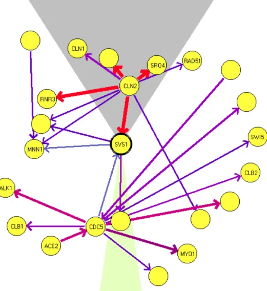
FIG. 2. An example of the graphical display of Markov features. This graph shows a “local map” for the gene
SVS1. The width (and color) of edges corresponds to the computed condence level. An edge is directed if there is a
sufciently high condence in the order between the genes connected by the edge. This local map shows that CLN2
separates SVS1 from several other genes. Although there is a strong connection between CLN2 to all these genes,
there are no other edges connecting them. This indicates that, with high condence, these genes are conditionally
independent given the expression level of CLN2.
4.1. Robustness analysis
We performed a number of tests to analyze the statistical signicance and robustness of our procedure. Some of these tests were carried out on a smaller data set with 250 genes for computational reasons.
To test the credibility of our condence assessment, we created a random data set by randomly permuting the order of the experiments independently for each gene. Thus for each gene the order was random, but the composition of the series remained unchanged. In such a data set, genes are independent of each other, and thus we do not expect to nd “real” features. As expected, both order and Markov relations in the random data set have signicantly lower condence. We compare the distribution of condence estimates between the original data set and the randomized set in Figure 3. Clearly, the distribution of condence estimates in the original data set have a longer and heavier tail in the high condence region. In the linear-Gaussian model we see that random data does not generate any feature with condence above 0.3. The multinomial model is more expressive and thus susceptible to over-tting. For this model, we see a smaller gap between the two distributions. Nonetheless, randomized data does not generate any feature with condence above 0.8, which leads us to believe that most features that are learned in the original data set with such condence are not artifacts of the bootstrap estimation.
M ar ko v O rd er M ul ti no m ia l 0 20 0 40 0 60 0 80 0 10 00 12 00 14 00 0. 2 0. 3 0. 4 0 .5 0. 6 0. 7 0. 8 0. 9 1 0 50 10 0 15 0 20 0 25 0 0. 2 0. 3 0. 4 0. 5 0. 6 0. 7 0. 8 0. 9 1 Fea tur es wit h C onf ide nce ab ove L in ea r-G au ss ia n 0. 2 0. 3 0. 4 0. 5 0. 6 0. 7 0. 8 0. 9 1 0 5 00 10 00 15 00 20 00 25 00 30 00 35 00 40 00 0 10 0 20 0 30 0 40 0 50 0 0. 2 0. 3 0. 4 0. 5 0. 6 0. 7 0. 8 0. 9 1 R an do m R ea l Fea tur es wit h C onf ide nce ab ove 0 20 00 40 00 60 00 80 00 10 00 0 12 00 0 14 00 0 0. 2 0. 4 0. 6 0. 8 1 Fea tur es wit h C onf ide nce ab ove 0 20 0 40 0 60 0 80 0 10 00 0. 2 0. 4 0. 6 0. 8 1 R an do m R ea l F IG .3 . P lo ts of ab un da nc e of fe at ur es w it h di ff er en t co nþ de nc e le ve ls fo r th e ce ll cy cl e da ta se t (s ol id lin e) , an d th e ra nd om iz ed da ta se t (d ot te d li ne ). T he x -a xi s de no te s th e co nþ de nc e th re sh ol d, an d th e y -a xi s de no te s th e nu m be r of fe at ur es w it h co nþ de nc e eq ua l or hi gh er th an th e co rr es po nd in g x -v al ue . T he gr ap hs on th e le ft co lu m n sh ow M ar ko v fe at ur es , an d th e on es on th e ri gh t co lu m n sh ow O rd er fe at ur es . T he to p ro w de sc ri be s fe at ur es fo un d us in g th e m ul ti no m ia l m od el , an d th e bo tt om ro w de sc ri be s fe at ur es fo un d by th e li ne ar -G au ss ia n m od el . In se t in ea ch gr ap h is a pl ot of th e ta il of th e di st ri bu ti on .
Order relations Markov relations 0 0.2 0.4 0.6 0.8 1 0 0.1 0.2 0.3 0.4 0.5 0.6 0.7 0.8 0.9 1 0 0.2 0.4 0.6 0.8 1 0 0.1 0.2 0.3 0.4 0.5 0.6 0.7 0.8 0.9 1
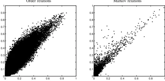
FIG. 4. Comparison of condence levels obtained in two data sets differing in the number of genes, on the multinomial
experiment. Each relation is shown as a point, with thex-coordinate being its condence in the the 250 genes data
set and they-coordinate the condence in the 800 genes data set. The leftgure shows order relation features, and
the rightgure shows Markov relation features.
To test the robustness of our procedure for extracting dominant genes, we performed a simulation study. We created a data set by sampling 80 samples from one of the networks learned from the original data. We then applied the bootstrap procedure on this data set. We counted the number of descendents of each node in the synthetic network and ordered the variables according to this count. Of the 10 top dominant genes learned from the bootstrap experiment, 9 were among the top 30 in the real ordering.
Since the analysis was not performed on the wholeS. cerevisiaegenome, we also tested the robustness of our analysis to the addition of more genes, comparing the condence of the learned features between the 800-gene data set and a smaller 250-gene data set that contains genes appearing in eight major clusters described by Spellmanet al.(1998). Figure 4 compares feature condence in the analysis of the two data sets for the multinomial model. As we can see, there is a strong correlation between condence levels of the features between the two data sets. The comparison for the linear-Gaussian model gives similar results.
A crucial choice for the multinomial experiment is the threshold level used for discretization of the expression levels. It is clear that by setting a different threshold we would get different discrete expression patterns. Thus, it is important to test the robustness and sensitivity of the high-condence features to the choice of this threshold. This was tested by repeating the experiments using different thresholds. The comparison of how the change of threshold affects the condence of features show a denite linear tendency in the condence estimates of features between the different discretization thresholds (graphs not shown). Obviously, this linear correlation gets weaker for larger threshold differences. We also note that order relations are much more robust to changes in the threshold than are Markov relations.
A valid criticism of our discretization method is that it penalizes genes whose natural range of variation is small: since we use axed threshold, we would not detect changes in such genes. A possible way to avoid this problem is tonormalize the expression of genes in the data. That is, we rescale the expression level of each gene so that the relative expression level has the same mean and variance for all genes. We note that analysis methods that usePearson correlationto compare genes, such as those of Ben-Doret al. (1999) and Eisenet al.(1999), implicitly perform such a normalization.4 When we discretize a normalized data set, we are essentially rescaling the discretization factor differently for each gene, depending on its variance in the data. We tried this approach with several discretization levels, and got results comparable
4An undesired effect of such a normalization is the amplication of measurement noise. If a gene hasxed expression
levels across samples, we expect the variance in measured expression levels to be noise either in the experimental conditions or the measurements. When we normalize the expression levels of genes, we lose the distinction between
such noise and true (i.e., signicant) changes in expression levels. In the Spellmanet al.data set we can safely assume
Order relations Markov relations 0 0.2 0.4 0.6 0.8 1 0 0.1 0.2 0.3 0.4 0.5 0.6 0.7 0.8 0.9 1 0 0.2 0.4 0.6 0.8 1 0 0.1 0.2 0.3 0.4 0.5 0.6 0.7 0.8 0.9 1
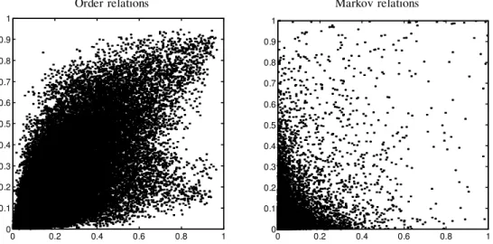
FIG. 5. Comparison of condence levels between the multinomial experiment and the linear-Gaussian experiment.
Each relation is shown as a point, with thex-coordinate being its condence in the multinomial experiment, and the
y-coordinate its condence in the linear-Gaussian experiment. The leftgure shows order relation features, and the
rightgure shows Markov relation features.
to our original discretization method. The 20 top Markov relations highlighted by this method were a bit different, but interesting and biologically sensible in their own right. The order relations were again more robust to the change of methods and discretization thresholds. A possible reason is that order relations depend on the network structure in a global manner and thus can remain intact even after many local changes to the structure. The Markov relation, being a local one, is more easily disrupted. Since the graphs learned are extremely sparse, each discretization method “highlights” different signals in the data, which are re ected in the Markov relations learned.
A similar picture arises when we compare the results of the multinomial experiment to those of the linear-Gaussian experiment (Figure 5). In this case, there is virtually no correlation between the Markov relations found by the two methods, while the order relations show some correlation. This supports our assumption that the two methods highlight different types of connections between genes.
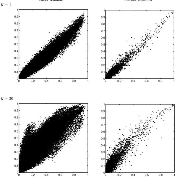
Finally, we consider the effect of the choice of prior on the learned features. It is important to ensure that the learned features are not simply artifacts of the chosen prior. To test this, we repeated the multinomial experiment with different values of K, the effective sample size, and compared the learned condence levels to those learned with the default value used forK, which was 5. This was done using the 250-gene data set and discretization level of 0.5. The results of these comparisons are shown in Figure 6. As can be seen, the condence levels obtained with a K value of 1 correlate very well with those obtained with the defaultK, while when settingK to 20 the correlation is weaker. This suggests that both 1 and 5 are low enough values compared to the data set size of 76, making the prior’s affect on the results weak. An effective sample size of 20 is high enough to make the prior’s effect noticeable. Another aspect of the prior is the prior network used. In all the experiments reported here, we used the empty network with uniform distribution parameters as the prior network. As our prior is noninformative, keeping down its effect is desired. It is expected that once we use more informative priors (by incorporating biological knowledge, for example) and stronger effective sample sizes, the obtained results will be biased more toward our prior beliefs.
In summary, although many of the results we report below (especially order relations) are stable across the different experiments discussed in the previous paragraph, it is clear that our analysis is sensitive to the choice of local model and, in the case of the multinomial model, to the discretization method. It is probably less sensitive to the choice of prior, as long as the effective sample size is small compared to the data set size. In all the methods we tried, our analysis found interesting relationships in the data. Thus, one challenge is to nd alternative methods that can recover all these relationships in one analysis. We are currently working on learning networks with semi-parametric density models (Friedman and Nachman, 2000; Hoffman and Tresp, 1996) that would circumvent the need for discretization on one hand and allow nonlinear dependency relations on the other.
Order relations Markov relations K5 1 0 0.2 0.4 0.6 0.8 1 0 0.1 0.2 0.3 0.4 0.5 0.6 0.7 0.8 0.9 1 0 0.2 0.4 0.6 0.8 1 0 0.1 0.2 0.3 0.4 0.5 0.6 0.7 0.8 0.9 1 K5 20 0 0.2 0.4 0.6 0.8 1 0 0.1 0.2 0.3 0.4 0.5 0.6 0.7 0.8 0.9 1 0 0.2 0.4 0.6 0.8 1 0 0.1 0.2 0.3 0.4 0.5 0.6 0.7 0.8 0.9 1
FIG. 6. Comparison of condence levels between runs using different parameter priors. The difference in the priors
is in the effective sample size,K. Each relation is shown as a point, with thex-coordinate being its condence in a
run withK5 5, and they-coordinate its condence in a run withK5 1 (top row) andK5 20 (bottom row). The
leftgure shows order relation features, and the rightgure shows Markov relation features. All runs are on the 250
gene set, using discretization with threshold level 0.5.
4.2. Biological analysis
We believe that the results of this analysis can be indicative of biological phenomena in the data. This is conrmed by our ability to predict sensible relations between genes of known function. We now examine several consequences that we have learned from the data. We consider, in turn, the order relations and Markov relations found by our analysis.
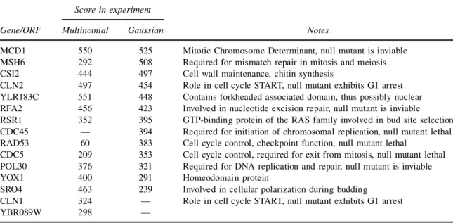
4.2.1. Order relations. The most striking feature of the high-condence order relations, is the existence ofdominant genes. Out of all 800 genes, only a few seem to dominate the order (i.e., appear before many genes). The intuition is that these genes are indicative of potential causal sources of the cell-cycle process. Let Co.X; Y / denote the condence in X being an ancestor of Y. We dene the dominance score of X asPY;C
o.X;Y />tCo.X; Y /
k;using the constantkfor rewarding high condence features and the threshold
t to discard low condence ones. These dominant genes are extremely robust to parameter selection for both t and k, the discretization cutoff of Section 3.5, and the local probability model used. A list of the highest-scoring dominating genes for both experiments appears in Table 1.
Table1. List of Dominant Genes in the Ordering Relations1
Score in experiment
Gene/ORF Multinomial Gaussian Notes
MCD1 550 525 Mitotic Chromosome Determinant, null mutant is inviable
MSH6 292 508 Required for mismatch repair in mitosis and meiosis
CSI2 444 497 Cell wall maintenance, chitin synthesis
CLN2 497 454 Role in cell cycle START, null mutant exhibits G1 arrest
YLR183C 551 448 Contains forkheaded associated domain, thus possibly nuclear
RFA2 456 423 Involved in nucleotide excision repair, null mutant is inviable
RSR1 352 395 GTP-binding protein of the RAS family involved in bud site selection
CDC45 — 394 Required for initiation of chromosomal replication, null mutant lethal
RAD53 60 383 Cell cycle control, checkpoint function, null mutant lethal
CDC5 209 353 Cell cycle control, required for exit from mitosis, null mutant lethal
POL30 376 321 Required for DNA replication and repair, null mutant is inviable
YOX1 400 291 Homeodomain protein
SRO4 463 239 Involved in cellular polarization during budding
CLN1 324 — Role in cell cycle START, null mutant exhibits G1 arrest
YBR089W 298 —
1Included are the top 10 dominant genes for each experiment.
Inspection of the list of dominant genes reveals quite a few interesting features. Among them are genes directly involved in initiation of the cell cycle and its control. For example, CLN1, CLN2, CDC5, and RAD53 whose functional relation has been established (Cvrckova and Nasmyth, 1993; Drebot et al., 1993). The genes MCD1, RFA2, CDC45, RAD53, CDC5, and POL30 were found to be essential (Guacci et al., 1997). These are clearly key genes in essential cell functions. Some of them are components of prereplication complexes(CDC45,POL30). Others (like RFA2,POL30, and MSH6) are involved in DNA repair. It is known that DNA repair is associated with transcription initiation, and DNA areas which are more active in transcription are also repaired more frequently (McGregor, 1999; Tornaletti and Hanawalk, 1999). Furthermore, a cell cycle control mechanism causes an abort when the DNA has been improperly replicated (Eisen and Lucchesi, 1998).
Most of the dominant genes encode nuclear proteins, and some of the unknown genes are also potentially nuclear (e.g., YLR183C contains a forkhead-associated domain which is found almost entirely among nuclear proteins). A few nonnuclear dominant genes are localized in the cytoplasm membrane (SRO4 and RSR1). These are involved in the budding and sporulation processes which have an important role in the cell cycle. RSR1 belongs to the RAS family of proteins, which are known as initiators of signal transduction cascades in the cell.
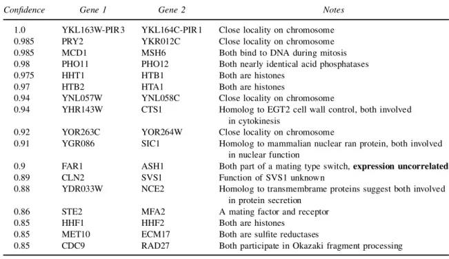
4.2.2. Markov relations. We begin with an analysis of the Markov relations in the multinomial ex-periment. Inspection of the top Markov relations reveals that most are functionally related. A list of the top scoring relations can be found in Table 2. Among these, all those involving two known genes make sense biologically. When one of the ORFs is unknown, careful searches using Psi-Blast (Altschulet al., 1997), Pfam (Sonnhammeret al., 1998), and Protomap (Yonaet al., 1998) can revealrm homologies to proteins functionally related to the other gene in the pair. For example YHR143W, which is paired to the endochitinase CTS1, is related to EGT2—a cell-wall-maintenance protein. Several of the unknown pairs are physically adjacent on the chromosome and thus presumably regulated by the same mechanism (see Blumenthal (1998)), although special care should be taken for pairs whose chromosomal location overlap on complementary strands, since in these cases we might see an artifact resulting from cross-hybridization. Such an analysis raises the number of biologically sensible pairs to nineteen out of the twenty top relations. Some interesting Markov relations were found that are beyond the limitations of clustering techniques. Among the high-condence Markov relations, one cannd examples of conditional independence, i.e., a group of highly correlated genes whose correlation can be explained within our network structure. One such example involves the genes CLN2,RNR3,SVS1,SRO4, and RAD51. Their expression is correlated, and in Spellman et al. (1998) they all appear in the same cluster. In our network CLN2 is with high condence a parent of each of the other 4 genes, while no links are found between them (see Figure 2). This agrees with biological knowledge: CLN2 is a central and early cell cycle control, while there is
Table2. List of Top Markov Relations, Multinomial Experiment
Condence Gene 1 Gene 2 Notes
1.0 YKL163W-PIR3 YKL164C-PIR1 Close locality on chromosome
0.985 PRY2 YKR012C Close locality on chromosome
0.985 MCD1 MSH6 Both bind to DNA during mitosis
0.98 PHO11 PHO12 Both nearly identical acid phosphatases
0.975 HHT1 HTB1 Both are histones
0.97 HTB2 HTA1 Both are histones
0.94 YNL057W YNL058C Close locality on chromosome
0.94 YHR143W CTS1 Homolog to EGT2 cell wall control, both involved
in cytokinesis
0.92 YOR263C YOR264W Close locality on chromosome
0.91 YGR086 SIC1 Homolog to mammalian nuclear ran protein, both involved
in nuclear function
0.9 FAR1 ASH1 Both part of a mating type switch,expression uncorrelated
0.89 CLN2 SVS1 Function of SVS1 unknown
0.88 YDR033W NCE2 Homolog to transmembrame proteins suggest both involved
in protein secretion
0.86 STE2 MFA2 A mating factor and receptor
0.85 HHF1 HHF2 Both are histones
0.85 MET10 ECM17 Both are sulte reductases
0.85 CDC9 RAD27 Both participate in Okazaki fragment processing
no clear biological relationship between the others. Some of the other Markov relations are intercluster pairing genes with low correlation in their expression. One such regulatory link is FAR1–ASH1: both proteins are known to participate in a mating-type switch. The correlation of their expression patterns is low and Spellmanet al.(1998) cluster them into different clusters. When looking further down the list for pairs whose Markov relation condence is high relative to their correlation, interesting pairs surface, for example, SAG1 and MF-ALPHA-1, a match between the factor that induces the mating process and an essential protein that participates in the mating process. Another match is LAC1 and YNL300W. LAC1 is a GPI transport protein and YNL300W is most likely modied by GPI (based on sequence homology).
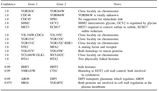
The Markov relations from the Gaussian experiment are summarized in Table 3. Since the Gaussian model focuses on highly correlated genes, most of the high-scoring genes are tightly correlated. When we checked the DNA sequence of pairs of physically adjacent genes at the top of Table 3, we found that there is signicant overlap. This suggests that these correlations are spurious and due to cross hybridization. Thus, we ignore the relations with the highest score. However, in spite of this technical problem, few of the pairs with a condence >0:8 can be discarded as biologically false.
Some of the relations are robust and also appear in the multinomial experiment (e.g., STE2–MFA2, CST1–YHR143W). Most interesting are the genes linked through regulation. These include: SHM2 which converts glycine that regulates GCV2 and DIP5 which transports glutamate which regulates ARO9. Some pairs participate in the same metabolic process, such as: CTS1–YHR143 and SRO4–YOL007C, all which participate in cell wall regulation. Other interesting high-condence (>0:9) examples are: OLE1–FAA4 linked through fatty acid metabolism, STE2–AGA2 linked through the mating process, and KIP3–MSB1, both playing a role in polarity establishment.
5. DISCUSSION AND FUTURE WORK
In this paper we presented a new approach for analyzing gene expression data that builds on the theory and algorithms for learning Bayesian networks. We described how to apply these techniques to gene expression data. The approach builds on two techniques that were motivated by the challenges posed by this domain: a novel search algorithm (Friedman, Nachman, and Pe’er, 1999) and an approach for estimating statistical condence (Friedman, Goldszmidt, and Wyner, 1999). We applied our methods to the real expression data of Spellman et al. (1998). Although, we did not use any prior knowledge, we managed to extract many biologically plausible conclusions from this analysis.
Table3. List of Top Markov Relations, Gaussian Experiment1
Condence Gene 1 Gene 2 Notes
1.0 YOR263C YOR264W Close locality on chromosome
1.0 CDC46 YOR066W YOR066W is totally unknown
1.0 CDC45 SPH1 No suggestion for immediate link
1.0 SHM2 GCV2 SHM2 interconverts glycine, GCV2 is regulated by glycine
1.0 MET3 ECM17 MET3 required to convert sulfate to sulde, ECM17
sulte reductase
1.0 YJL194W-CDC6 YJL195C Close locality on chromosome
1.0 YGR151C YGR152C Close locality on chromosome
1.0 YGR151C YGR152C-RSR1 Close locality on chromosome
1.0 STE2 MFA2 A mating factor and receptor
1.0 YDL037C YDL039C Both homologs to mucin proteins
1.0 YCL040W-GLK1 WCL042C Close locality on chromosome
1.0 HTA1 HTA2 Two physically linked histones
: : :
0.99 HHF2 HHT2 both histones
0.99 YHR143W CTS1 Homolog to EGT2 cell wall control, both involved
in cytokinesis
0.99 ARO9 DIP5 DIP5 transports glutamate which regulates ARO9
0.975 SRO4 YOL007C Both proteins are involved in cell wall regulation at the
plasma membrane 1The table skips over 5 additional pairs with which close locality.
Our approach is quite different from the clustering approach used by Alonet al.(1999), Ben-Doret al. (1999), Eisen et al. (1999), Michaels et al. (1998), and Spellman et al. (1998) in that it attempts to learn a much richer structure from the data. Our methods are capable of discovering causal relationships, interactions between genes other than positive correlation, andner intracluster structure. We are currently developing hybrid approaches that combine our methods with clustering algorithms to learn models over “clustered” genes.
The biological motivation of our approach is similar to the work on inducing genetic networks from data (Akutsuet al., 1998; Chenet al., 1999; Somogyiet al., 1996; Weaveret al., 1999). There are two key differences: First, the models we learn have probabilistic semantics. This betterts the stochastic nature of both the biological processes and noisy experiments. Second, our focus is on extracting features that are pronounced in the data, in contrast to current genetic network approaches that attempt tond a single model that explains the data.
We emphasize that the work described here represents a preliminary step in a longer-term project. As we have seen above, there are several points that require accurate statistical tools and more efcient algorithms. Moreover, the exact biological conclusions one can draw from this analysis are still not well understood. Nonetheless, we view the results described in Section 4 as denitely encouraging.
We are currently working on improving methods for expression analysis by expanding the framework described in this work. Promising directions for such extensions are: (a) developing the theory for learning local probability models that are suitable for the type of interactions that appear in expression data; (b) improving the theory and algorithms for estimating condence levels; (c) incorporating biological knowledge (such as possible regulatory regions) as prior knowledge to the analysis; (d) improving our search heuristics; (e) learning temporal models, such as Dynamic Bayesian Networks (Friedman et al., 1998), from temporal expression data, and (f) developing methods that discover hidden variables (e.g., protein activation).
Finally, one of the most exciting longer-term prospects of this line of research is discovering causal patterns from gene expression data. We plan to build on and extend the theory for learning causal relations from data and apply it to gene expression. The theory of causal networks allows learning from both observational and interventional data, where the experiment intervenes with some causal mechanisms of the observed system. In the gene expression context, we can model knockout/over-expressed mutants as such interventions. Thus, we can design methods that deal with mixed forms of data in a principled manner (see Cooper and Yoo (1999) for recent work in this direction). In addition, this theory can provide