A Generalized Inflated Geometric Distribution

(1)

Marshall University

Marshall Digital Scholar

Theses, Dissertations and Capstones

2015

A Generalized Inflated Geometric Distribution

Ram Datt Joshi

[email protected]

Follow this and additional works at:

http://mds.marshall.edu/etd

Part of the

Statistical Models Commons

, and the

Statistical Theory Commons

This Thesis is brought to you for free and open access by Marshall Digital Scholar. It has been accepted for inclusion in Theses, Dissertations and

Capstones by an authorized administrator of Marshall Digital Scholar. For more information, please [email protected].

Recommended Citation

(2)

A GENERALIZED INFLATED GEOMETRIC DISTRIBUTION

A thesis submitted to the Graduate College of

Marshall University In partial fulfillment of the requirements for the degree of

Master of Arts in Mathematics

by Ram Datt Joshi

Approved by

Dr. Avishek Mallick, Committee Chairperson Dr. Laura Adkins

Dr. Alfred Akinsete

Marshall University May 2015

(3)

ACKNOWLEDGEMENTS

First, I would like to express my sincere thanks to my thesis adviser Dr. Avishek Mallick for his continuous support and guidance throughout the entire project. His infectious enthusiasm and unlimited zeal has always pushed me forward to the completion of the thesis. Without his support, this work would never have been in this form. Besides, he is the one who challenged me the most and pushed me the hardest from his courses in class from the beginning of my master’s program at Marshall. I take the opportunity to say that he prepared me thoroughly for a doctoral program.

I would like to thank my committee members Dr. Alfred Akinsete and Dr. Laura Adkins. Dr. Akinsete is the one who always encouraged and guided me whenever I was in need of his guidance. He provided the easy and the best solution for whatever I used to reach him at. I am always grateful to his generosity and support. On the other hand, Dr. Adkins always has been eager to know about the progress and updates throughout my work. She always encouraged me for the com-pletion of my thesis as well as my studies throughout my stay at Marshall. I am fortunate to be a student in one of her classes at Marshall where I learned a lot from her incredible Biostatistics class.

In addition, a special thank you to Dr. Rubin Gerald who taught me throughout my last year in his statistics classes. I learned many things from his classes which have been useful for the comple-tion of this thesis. Moreover, he has been a constant source of inspiracomple-tion towards the complecomple-tion my masters degree at Marshall.

I would like to thank Dr. Basant Karna who as my mentor, helped and guided me throughout in every possible way. I am grateful for his care and guidance in every step I seek help from him throughout my time at Marshall. Without his support, life would not have been so easier. The other faculty that I never forget to mention is Dr. Ari Aluthge. He has not only prepared me in his Advanced Calculus course, but also helped me to go to the advanced doctoral program by writing letters of recommendation and giving me the courage to go ahead at the time of necessity.

(4)

A sincere thank goes to Dr. Carl Mummert for he has been the constant source of motivation towards the completion of my masters degree at Marshall. He is the professor who always listen every student carefully and he is fond of helping others.

I would like to thank the whole Department of Mathematics at Marshall University, for every member associated with the department has helped me directly or indirectly for the completion of my thesis in different possible ways.

At last but not the least, I would like to thank my parents and my wife-Saru, who always have been the source of motivation and inspiration throughout. They have been apprehensive about my study goals and my health condition. Without their blessings and prayers, this work would not have come into existence. I am thankful for my own health condition as well.

(5)

CONTENTS

List of Figures . . . v

List of Tables . . . vii

Abstract . . . viii

Chapter 1 Introduction . . . 1

Chapter 2 Estimation of Model Parameters . . . 5

2.1 Method of Moments Estimation . . . 5

2.2 Maximum Likelihood Estimation . . . 7

Chapter 3 Simulation Study . . . 10

3.1 The ZIG Distribution . . . 10

3.2 The ZOIG Distribution . . . 13

3.3 The ZOTIG Distribution . . . 16

Chapter 4 Application of GIG Distribution . . . 26

4.1 An Example . . . 26

4.2 Conclusion . . . 27

Appendix A Algebraic Solutions for the Method of Moments Estimators . . . 29

Appendix B Letter from Institutional Research Board . . . 31

References . . . 32

(6)

LIST OF FIGURES

3.1 Plots of the SBias and SMSE of the CMMEs and MLEs of π1 and p (from ZIG

distribution) for n= 25 . . . 11

3.2 Plots of the SBias and SMSE of the CMMEs and MLEs of π1 and p (from ZIG

3.3 Plots of the SBias and SMSE of the CMMEs and MLEs ofπ1,π2 andp(from ZOIG

3.7 Plots of the SBias and SMSE of the CMMEs and MLEs of π1, π2, π3 and p (from

ZOTIG distribution) for n= 25 . . . 19

(7)

4.1 Plot of the observed frequencies compared to the estimated frequencies from the

(8)

LIST OF TABLES

(9)

ABSTRACT

A count data that have excess number of zeros, ones, twos or threes are commonplace in exper-imental studies. But these inflated frequencies at particular counts may lead to over dispersion and thus may cause difficulty in data analysis. So, to get appropriate results from them and to overcome the possible anomalies in parameter estimation, we may need to consider suitable inflated distribution.

In this thesis, we have considered a Swedish fertility dataset with inflated values at some par-ticular counts. Generally, Inflated Poisson or Inflated Negative Binomial distribution are the most common distributions for analyzing such data. Geometric distribution can be thought of as a spe-cial case of Negative Binomial distribution. Hence we have used a Geometric distribution inflated at certain counts, which we called Generalized Inflated Geometric distribution to analyze such data. The data set is analyzed, tested and compared using various tests and techniques to ensure the better performance of multi-point inflated Geometric distribution over the standard Geometric distribution.

The various tests and techniques used include comparing the parameters obtained through method of moment estimators and maximum likelihood estimators. The two types of estimators obtained from method of moment estimations and maximum likelihood estimation method, were compared using simulation study, and it is found after the analysis that the maximum likelihood estimators perform better.

(10)

CHAPTER 1 INTRODUCTION

A random variableX that counts the number of trials to obtain the rth success in a series of

independent and identical Bernoulli trials, is said to have a Negative Binomial distribution whose probability mass function (pmf) is given by

P(X =k) =P(k|p) = k−1 r−1 pr(1−p)k−r (1.1) wherer = 1,2,3, . . .;k=r, r+ 1, . . . and p >0.

The above distribution is also the “Generalized Power Series distribution” as mentioned in Johnson et al. (2005)[7]. Some writers, for instance Patil et al. (1984)[9], called this the “P´olya-Eggenberger distribution”, as it arises as a limiting form of Eggenberger and P´olya’s (1923)[3] urn model distribution. A special case of Negative Binomial Distribution is the Geometric distribution which can be defined in two different ways

Firstly, the probability distribution for a Geometric random variable X (where X being the number of independent and identical trials to get the first success) is given by

P(X =k|p) =        p(1−p)k−1 ifk= 1,2, . . . 0 otherwise. (1.2)

However, instead of counting the number of trials, if the random variableX counts the number

of failures before the first success, then it will result in the second type of Geometric distribution

which again is a special case of Negative Binomial distribution when r= 1 (first success) and its

pmf is given by P(X=k) =P(k|p) =        p(1−p)k ifk= 0,1,2, . . . 0 otherwise. (1.3)

(11)

distribution in (1.2). The above model in (1.3), henceforth referred to as “Geometric(p)” has

mean 1−p

p and variance

1−p

p2 and is the only distribution with non-negative integer support

that can be characterized by the “Memory-less property” or the “Markovian property”. Many other characterizations of this distribution can be found in Feller (1968, 1969) [4] [5]. The distribution occurs in many applications and some of them are indicated in the references below:

• The famous problem of Banach’s match boxes (Feller (1968)[4]);

• The runs of one plant species with respect to another in transects through plant populations

(Pielou (1962, 1963)[10][11]);

• A ticket control problem (Jagers (1973)[6]);

• A survillance system for congenital malformations (Chen (1978)[2]);

• The number of tosses of a fair coin before the first head (success) appears;

• The number of drills in an area before observing the first productive well by an oil

prospector.(Wackerly et al. (2008)[13]).

The Geometric model in (1.3) which is widely used for modeling count data may be inadequate for dealing with overdispersed as well as underdispersed count data. One such instance is the abundance of zero counts in the data, and (1.3) may be an inefficient model for such cases due to the presence of heterogeneity, which usually results in undesired over dispersion. Therefore, to overcome this situation, i.e., to explain or capture such heterogeneity, we consider a ‘two-mass

distribution’ by giving massπ to 0 counts, and mass (1−π) to the other class which follows

Geometric(p). The result of such a ’mixture distribution’ is called the ’Zero-Inflated Geometric’ (ZIG) distribution with the probability mass function

P(k|p, π) =        π+ (1−π)p ifk= 0 (1−π)P(k|p) ifk= 1,2, . . . (1.4)

where, p >0, andP(k|p) is given in (1.3). However the mixing parameterπ is chosen such that

(12)

distribution to be well defined for certain negative values of π, depending onp. Although the

mixing interpretation is lost whenπ <0, these values have a natural interpretation in terms of

zero-deflation, relative to a Geometric(p) model. Correspondingly,π >0 can be regarded as zero

inflation as discussed in Johnson et al. (2005)[7].

A further generalization of (1.4) can be obtained by inflating/deflating the Geometric

distribution at several specific values. To be precise, if the discrete random variableX is thought

to have inflated probabilities at the valuesk1, ...., km ∈ {0,1,2, ....}, then the following general

probability mass function can be considered:

P(k|p, πi,1≤i≤m) =          πi+ 1−Pm i=1 πi P(k|p) ifk=k1, k2, . . . , km 1−Pm i=1 πi P(k|p) ifk6=ki; 1≤i≤m (1.5)

wherek= 0,1,2, . . .;p >0 and πi’s are chosen in such a way that P(ki)∈(0,1) for all

i= 1,2, ..., min (1.5). For the remainder of this work, we will refer to (1.5) as the Generalized Inflated Geometric (GIG) distribution which is the main focus of this work.

We will consider some special cases of the (GIG) distribution such as Zero-One-Inflated

Geometric (ZOIG) distribution in the casek= 2 withk1 = 0 and k2 = 1 or Zero-One-Two

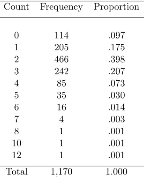
Inflated Geometric (ZOTIG) models. Similar type of Generalized Inflated Poisson (GIP) models have been considered by Melkersson and Rooth (2000)[8] to study a women’s fertility data of 1170 Swedish women of the age group 46-76 years (Table 1.1). This data set consists of the number of child(ren) per woman, who have crossed the childbearing age in the year 1991. They justified the Zero-Two Inflated Poisson distribution was the best to model it. However recently in his Master’s Thesis, Stewart (2014)[12] studied the same data set and found that a Zero-Two-Three Inflated Poisson (ZTTIP) distribution was a better fit.

Instead of using an Inflated Poisson model, we will consider fitting appropriate Inflated Geometric models to the data in Table 1.1. Now, which model is the best fit whether a GIG model with focus on counts (0, 1), i.e., ZOIG or a GIG model focusing on some other set {k1, k2, ..., km} is appropriate for the above data will be eventually decided by different model

(13)

Table 1.1: Observed number of children (=count) per woman

Count Frequency Proportion

0 114 .097 1 205 .175 2 466 .398 3 242 .207 4 85 .073 5 35 .030 6 16 .014 7 4 .003 8 1 .001 10 1 .001 12 1 .001 Total 1,170 1.000

estimation namely, the method of moments (MME), and the maximum likelihood estimation (MLE). In Chapter 3, we compare the performances of MMEs and MLEs for different GIG model parameters using simulation studies.

(14)

CHAPTER 2

ESTIMATION OF MODEL PARAMETERS

In this chapter, we estimate the parameters by two well known methods of parameter estimation namely the method of moment estimations and the method of maximum likelihood estimations.

2.1 Method of Moments Estimation (MME)

The easiest way to obtain estimators of the parameters is through the method of moments

estimation (MME). The rth raw moment of a random variableX following a GIG in (1.5) with

parameters π1, . . . , πm and p can be obtained from the following expression:

E[Xr] = ∞ X k=0 krP(k|p, πi,1≤i≤m) = m X i=1 k_irπi+ (1− m X i=1 πi) ∞ X k=0 krP(k|p) = m X i=1 k_irπi+ (1− m X i=1 πi)µ0r(p). (2.1)

whereµ0_r(p) is the therth raw moment of Geometric(p) and can be calculated easily by

differentiating its moment generating function (MGF) given by p

1−(1−p)et, i.e., µ0_r(p) = _dtdrr p 1−(1−p)et t=0.

Given a random sample X1, ...., Xn, i.e. independent and identically distributed (iid)

observations from the GIG distribution, we equate the sample moments with the corresponding population moments to get a system of (m+1) equations involving the (m+1) model parameters

p, π1, . . . , πm of the form m0_r= m X i=1 k_irπi+ 1− m X i=1 πi ! µ0_r(p) (2.2)

wherer = 1,2, . . . ,(m+ 1). Note that m0_r =Pn_j₌₁Xr

j/nis the rth raw sample moment. The

values ofπi, i= 1,2, ...., m, and p obtained by solving the system of equations (2.2) are denoted

by ˆπ_i₍_{M M}₎ and ˆpM M respectively. The subscript “(MM)” indicates the MME approach. Note that

(15)

no such guarantee, as such we propose the corrected MME’s to ensure non-negativity of this moment estimator as

ˆ

pc_{M M} = ˆpM M truncated at 0 and 1 and ˆπci(M M)= ˆπi(M M) (2.3)

where ˆπc_i₍_{M M}₎ is the solution ofπi in (2.2) obtained after substituting ˆpM M.

Consider the case of ZIG distribution when m= 1 i.e., k1= 0, resulting into only two

parameters to estimate, i.e. π1 and p. The population mean and population variance in this

special case are obtained as:

E(X) = (1−π1)

(1−p)

p and V ar(X) = (1−π1){1 +π1(1−p)}

(1−p)

p2 (2.4)

Now, in order to obtain the method of moments estimators, we can equate the preceding mean

and variance with sample mean ( ¯X) and sample variance (s2_{) respectively. This is an alternative}

approach to estimate the parameters instead of dealing with the sample raw moments. Hence we obtain, (1−π1) (1−p) p = ¯X (1−π1){1 +π1(1−p)} (1−p) p2 =s 2 _(2.5)

Solving the above equations simultaneously for pand π1, we get, ˆpcM M =

2 ¯X (s2_{+ ¯}_X_{+ ¯}_X2₎ and ˆ π₁₍c_{M M}₎= s 2₋_X_¯ ₋_X_¯2 s2₋_X¯ _{+ ¯}_X2.

Now let us consider another special case of GIG, the Zero-One Inflated Geometric (ZOIG) distribution, i.e., m= 2 andk1= 0 and k2= 1. It has three parameters π1,π2 and p and to

(16)

population moments and we thus obtain the following system of equations: m0₁ = π2+ (1−π1−π2) (1−p) p m0₂ = π2+ (1−π1−π2) (p2−3p+ 2) p2 m0₃ = π2+ (1−π1−π2) (1−p)(p2−6p+ 6) p3 (2.6)

Similarly, another special case of GIG is the Zero-One-Two Inflated Geometric (ZOTIG)

distribution. Here we have four parameters π1,π2,π3 and pto estimate. This is done by solving

the following system of four equations obtained by equating the first four raw sample moments with their corresponding population moments to have,

m0₁ = π2+ 2π3+ (1−π1−π2−π3) (1−p) p m0₂ = π2+ 4π3+ (1−π1−π2−π3) (1−p)(2−p) p2 m0₃ = π2+ 8π3+ (1−π1−π2−π3) (1−p)(p2−6p+ 6) p3 m0₄ = π2+ 16π3+ (1−π1−π2−π3) (1−p)(2−p)(p2−12p+ 12) p4 (2.7)

Algebraic solutions to these systems of equations in (2.6) and (2.7) are obtained by using Mathematica and are given in Appendix (A). We note that these solutions may not fall in the feasible regions of the parameter space, so we put appropriate restrictions to these solutions as discussed for the ZIG distribution to obtain the corrected MMEs.

2.2 Maximum Likelihood Estimation (MLE)

In this section, we discuss the approach of estimating our parameters by the method of Maximum

Likelihood Estimation(MLE). Based on the random sampleX= (X1, X2, . . . , Xn), we define the

likelihood function L=L(p, πi,1≤i≤m| X) as follows. LetYi = the number of observations at

ki with inflated probability, i.e., ifI is an indicator function, thenYi=Pn_j₌₁I(Xj =ki),

1≤i≤m, which meansYi is the total number of observed counts atki. Also, let Y.=Pm_i₌₁Yi=

(17)

(n−Y.) is the total number of non-inflated observations. Then, L= m Y i=1 {πi+ (1− m X l=1 πl)P(ki |p)}Yi Y Xj6=ki {(1− m X l=1 πl)P(Xj|p)} = m Y i=1 {πi+ (1− m X l=1 πl)P(ki |p)}Yi(1− m X l=1 πl)(n−Y.) Y Xj6=ki P(Xj|p) (2.8)

The log likelihood function l= lnL is given by

l= m X i=1 Yiln{πi+ (1− m X l=1 πl)P(ki|p)}+ (n−Y.) ln(1− m X l=1 πl) + X Xj6=ki lnP(Xj |p) But we have, X Xj6=ki lnP(Xj |p) = (n−Y.) lnp+ ln(1−p)( n X j=1 Xj− m X l=1 klYl)

hence the log likelihood function becomes

l= m X i=1 Yi ln{πi+ (1− m X l=1 πl)P(ki|p)}+ (n−Y.) ln(1− m X l=1 πl) + (n−Y.) lnp+ ln(1−p)( n X j=1 Xj− m X l=1 klYl) (2.9)

Now to obtain the MLEs, we maximizel in (2.9) with respect to the parameters πi, 1≤i≤m,

and p over the appropriate parameter space. Differentiatingl partially w.r.t the parameters and

setting them equal to zero yields the following system of likelihood equations or score equations.

∂l ∂πi = Yi {πi+ (1−Pml=1πl)P(ki|p)} − m X i=1 YiP(ki|p) {πi+ (1−Pml=1πl)P(ki|p)} − (n−Y.) (1−Pm_l₌₁πl) = 0, ∀i= 1, . . . , m; ∂l ∂p = m X i=1 Yi(1−Pm_l₌₁πl)P(p)(ki|p) {πi+ (1−Pml=1πl)P(ki|p)} +(n−Y.) p − (nX¯ −Pm_l₌₁klYl) (1−p) = 0 (2.10) where, P(p)(ki|p) = (∂/∂p)P(ki|p).

At this point, we can not say which of these two estimation techniques (MME or MLE) provide overall better estimators.To the best of our knowledge, no comparative study has been reported in

(18)

literature. Further we do not have any closed form expressions for these estimators which makes it even more difficult to compare their performance. Therefore, we conduct simulation studies in the next chapter which can provide some guidance about their performances.

(19)

CHAPTER 3 Simulation Study

We have considered the following three cases for our simulation study:

(i) m= 1, k1 = 0 (Zero Inflated Geometric (ZIG) distribution)

(ii) m= 2, k1= 0, k2= 1 (Zero-One Inflated Geometric (ZOIG) distribution)

(ii) m= 3, k1= 0, k2= 1, k3= 2 (Zero-One-Two Inflated Geometric (ZOTIG) distribution)

For each model mentioned above, we generate random data X1, ..., Xn from the distribution

(with given parameter values) N = 10,000 times. Let us denote a parameter (either πi orp) by

the generic notationθ. The parameter θ is estimated by two possible estimators ˆθ(_{M M}c) (the

corrected MME) and ˆθM L (the MLE). At thelth replication, 1≤l≤N, the estimates of θ are

ˆ

θ(_{M M}c)(l) and ˆθ(_{M L}l) respectively. Then the standardized bias (called ‘SBias’) and standardized mean squared error (called ‘SMSE’) are defined and approximated as below

SBias(ˆθ) =E(ˆθ−θ)/θ≈ { N X l=1 (ˆθ(l)−θ)/θ}/N SMSE(ˆθ) =E(ˆθ−θ)2/θ2≈ { N X l=1 (ˆθ(l)−θ)2/θ2}/N (3.1)

Note that ˆθ will be replaced by ˆθ_{M M}(c) and ˆθM L in our simulation study. Further observe that we

are using SBias and SMSE instead of the actual Bias and MSE, because the standardized versions provide more information. An error of magnitude 0.01 in estimating a parameter with true value 1.00 is more severe than a situation where the parameter’s true value is 10.0. This fact is revealed through SBias and/or SMSE more than the actual bias and/or MSE.

3.1 The ZIG Distribution

In our simulation study for the Zero Inflated Geometric (ZIG) distribution, we fix p= 0.2 and

varyπ1 from 0.1 to 0.8 with an increment of 0.1 for n = 25 and n = 50. The constrained

optimization algorithm “L-BFGS-B” (Byrd et al. (1995))[1] is implemented in R programming

(20)

the corrected MMEs are obtained by solving a system of equations and imposing appropriate restrictions on the parameters. In order to compare the performances of the MLEs with that of the CMMEs, we plot the standardized biases (SBias) and standardized MSE (SMSE) of these

estimators obtained over the allowable range ofπ1. The SBias and SMSE plots are presented in

Figure(3.1) and Figure(3.2) for sample sizes 25 and 50 respectively.

● ● ● ● ● ● ● ● 0.1 0.2 0.3 0.4 0.5 0.6 0.7 0.8 −0.15 −0.05 0.00 0.05 π1 (a) SBias ● ● ● ● _● ● ● ● 0.1 0.2 0.3 0.4 0.5 0.6 0.7 0.8 0.0 0.2 0.4 0.6 0.8 1.0 π1 (c) SMSE ● ● ● ● ● ● ● ● 0.1 0.2 0.3 0.4 0.5 0.6 0.7 0.8 0.00 0.05 0.10 0.15 p (b) SBias ● ● ● ● ● ● ● ● 0.1 0.2 0.3 0.4 0.5 0.6 0.7 0.8 0.00 0.05 0.10 0.15 p (d) SMSE

Figure 3.1: Plots of the absolute SBias and SMSE of the CMMEs and MLEs of π1 and p (from

ZIG distribution) plotted against π1 forp= 0.2 andn= 25. The solid line represents the SBias or

SMSE of the CMME. The dashed line represents the SBias or SMSE of the MLE. (a) Comparison

of SBias of π1 estimators. (b) Comparison of SBias of p estimators. (c) Comparison of SMSE of

π1 estimators. (d) Comparison of SMSE ofp estimators.

For the ZIG distribution withn= 25, from Figure 3.1(a) we see that MLE outperforms CMME

for all values ofπ1 with respect to SBias. Here MLE is almost unbiased for all values of π1

beyond 0.4. The SBias seems to be maximum for CMME at 0.2 and for MLE at around 0.1. In Figure 3.1(b), we again see that MLE uniformly outperforms the CMME and both are increasing

(21)

● ● ● ● ● ● ● ● 0.1 0.2 0.3 0.4 0.5 0.6 0.7 0.8 −0.15 −0.05 0.00 0.05 π1 (a) SBias ● ● ● ● _● ● ● ● 0.1 0.2 0.3 0.4 0.5 0.6 0.7 0.8 0.0 0.2 0.4 0.6 0.8 1.0 π1 (c) SMSE ● ● ● ● ● ● ● ● 0.1 0.2 0.3 0.4 0.5 0.6 0.7 0.8 0.00 0.05 0.10 0.15 p (b) SBias ● ● ● ● ● ● ● ● 0.1 0.2 0.3 0.4 0.5 0.6 0.7 0.8 0.00 0.05 0.10 0.15 p (d) SMSE

Figure 3.2: Plots of the absolute SBias and SMSE of the CMMEs and MLEs of π1 and p (from

ZIG distribution) plotted against π1 forp= 0.2 andn= 50. The solid line represents the SBias or

SMSE of the CMME. The dashed line represents the SBias or SMSE of the MLE. (a) Comparison

of SBias of π1 estimators. (b) Comparison of SBias of p estimators. (c) Comparison of SMSE of

(22)

after which they both seem to have nearly the same SMSE. For both MLE and CMME, the SMSE starts off at their highest values and then decreases rapidly until it reaches nearly zero. The SMSE of MLE consistently outperforms that of CMME in Figure 3.1(d). They both start off at their lowest values, and increase as values of π1 get higher.

Again MLEs outperform CMMEs with respect to both SBias and SMSE for sample size 50, as

exhibited by Figure 3.2. So we see for the ZIG distribution, the MLEs of the parametersπ1 and p

perform better than the CMMEs for all values of π1 we have considered.

3.2 The ZOIG Distribution

In the case of the Zero-One Inflated Geometric (ZOIG) distribution we have three parameters to consider, namelyπ1,π2 and p. For fixed p= 0.3 we varyπ1 and π2 one at a time for sample sizes

25 and 50. Figure 3.3 presents the six comparisons for ˆπ(₁₍c)_{M M}₎, ˆπ₂₍(c)_{M M}₎ and ˆp(₍c_{M M}) ₎ with ˆπ1(M L),

ˆ

π2(M L) and ˆp(M L) in terms of standardized bias and standardize MSE for n= 25, varying π1 from

0.1 to 0.5 and keeping π2 andλfixed at 0.15 and 0.3 respectively. Figure 3.4 shows the same for

n= 50.

In Figure 3.3(a), MLE outperforms CMME at all points with respect to SBias. SBias of MLE starts above zero and quickly becomes negative, whereas that of CMME is throughout negative.

In Figure 3.3(b), we see that the MLE is almost unbiased for all values ofπ1, and SBias of

CMME is always negative. Again in Figure 3.3(c), we see that MLE is essentially unbiased but

SBias of CMME is increasing with values ofpi1. In Figure 3.3(d), SMSE of CMME and MLE are

both decreasing, but SMSE of MLE stays below that of CMME. In Figures 3.3(e) and 3.3(f),

SMSE of MLE stays constant at 0.55 and 0.05 respectively for all permissible values of π1. Also

CMME performs way worse for both the cases.

In Figure 3.4, we observe similar performance as in Figure 3.3, i.e, MLEs of all the parameters

is outperforming CMMEs with respect to both SBias and SMSE for all considered values of pi1.

In our second scenario which is presented in Figures 3.5 and 3.6 for sample sizes 25 and 50

respectively, we vary π2 keepingπ1 and λfixed at 0.15 and 3 respectively. In Figures 3.5(a), we

see that both MLE and CMME are negatively biased, but MLE is always performing better that the CMME. However in Figure 3.5(b), MLE starts of with a positive bias and then becomes

(23)

● ● ● ● _● 0.1 0.2 0.3 0.4 0.5 −0.5 −0.3 −0.1 0.1 π1 (a) SBias ● ● ● ● _● 0.1 0.2 0.3 0.4 0.5 0.0 0.5 1.0 1.5 2.0 π1 (d) SMSE ● _● ● ● ● 0.1 0.2 0.3 0.4 0.5 −0.8 −0.4 0.0 π2 (b) SBias ● ● ● ● ● 0.1 0.2 0.3 0.4 0.5 0.0 0.5 1.0 1.5 π2 (e) SMSE ● ● ● ● ● 0.1 0.2 0.3 0.4 0.5 0.0 0.2 0.4 0.6 p (c) SBias ● ● ● ● ● 0.1 0.2 0.3 0.4 0.5 0.0 0.2 0.4 0.6 0.8 p (f) SMSE

Figure 3.3: Plots of the SBias and SMSE of the CMMEs and MLEs of π1, π2 and p (from ZOIG

distribution) by varying π1 for fixed π2 = 0.15, p = 0.3 and n = 25. The solid line represents

the SBias or SMSE of the corrected MME. The dashed line represents the SBias or SMSE of the

MLE. (a)-(c) Comparisons of SBiases ofπ1,π2 andp estimators respectively. (d)-(f) Comparisons

(24)

● ● ● ● ● 0.1 0.2 0.3 0.4 0.5 −0.5 −0.3 −0.1 0.1 π1 (a) SBias ● ● ● ● ● 0.1 0.2 0.3 0.4 0.5 0.0 0.5 1.0 1.5 2.0 π1 (d) SMSE ● ● ● ● ● 0.1 0.2 0.3 0.4 0.5 −0.8 −0.4 0.0 π2 (b) SBias ● ● ● _● ● 0.1 0.2 0.3 0.4 0.5 0.0 0.5 1.0 1.5 π2 (e) SMSE ● ● ● ● ● 0.1 0.2 0.3 0.4 0.5 0.0 0.2 0.4 0.6 p (c) SBias ● ● ● ● ● 0.1 0.2 0.3 0.4 0.5 0.0 0.2 0.4 0.6 0.8 p (f) SMSE

(25)

unbiased for π2 between 0.2 and 0.3 and eventually ends with a negative bias. SBias of CMME

stays throughout between -0.6 and -0.8. In Figure 3.5(c), we see that MLE outperforms MME throughout with respect to SBias. From Figures 3.5(d), 3.5(e) and 3.5(f), it is clear that MLE

outperforms MME with respect to SMSE for all permissible values ofπ2. Thus we observe that

the MLEs of the all three parameters perform better than the MMEs in terms of the both absolute SBias and SMSE.

In Figure 3.6, we observe similar performance as in Figure 3.5, i.e, MLEs of all the parameters is

outperforming CMMEs with respect to both SBias and SMSE for all values ofπ2 from 0.1 to 0.5.

3.3 The ZOTIG Distribution

For the Zero-One-Two Inflated Geometric (ZOTIG) distribution we have four parameters to consider, namelyπ1,π2,π3 and p. For fixed p= 3 we vary π1,π2, and π3 one at a time from 0.1

to 0.5 for sample sizes n= 25 and n= 50. Thus we have eight comparisons for ˆπ₁₍(c_{M M}) ₎, ˆπ(₂₍c)_{M M}₎, ˆ

π₃₍(c)_{M M}₎ and ˆp₍(c_{M M}) ₎ with ˆπ1(M L), ˆπ2(M L), ˆπ3(M L) and ˆp(M L). These comparisons in terms of

absolute standardized bias and standardize MSE are presented in Figures 3.7-3.12.

In the first scenario of ZOTIG distribution, which is presented in Figures 3.7 and 3.8, we vary

π1 keepingπ2,π3 and p fixed at 0.2, 0.2 and 0.3 respectively. From Figure 3.7(a, b, c, d), we see

that the CMMEs of all the four parameters perform consistently worse than the MLEs with

respect to SBias. However SBias of CMMEs and MLEs are same at π1 = 0.5. Also from parts (e,

f, g, h) in Figure 3.7 concerning the SMSE, we notice that the CMMEs of all the parameters perform consistently worse than the MLEs. But as in the case of SBias, we see that SMSE of

CMMEs and MLEs are same atπ1= 0.5. In Figure 3.8, for sample size 50 we again observe that

MLE of all the four parameters are outperforming CMME with respect to SBias and SMSE.

In our second scenario which is presented in Figures 3.9 and 3.10, we vary π2 keepingπ1,π3

and p fixed at 0.2, 0.2 and 0.3 respectively. We observe some interesting things in these plots.

From Figure 3.9 we see that MLE of bothπ1 and pis performing better upto π2= 0.3 with

respect to SBias but after that CMME is performing slightly better than MLE. Also MLE ofπ2 is

better till 0.3 but after that both MLE and CMME have the same SBias. However we see that the MLEs of all four parameters perform better than their CMME counterparts with respect to

(26)

● ● ● ● ● 0.1 0.2 0.3 0.4 0.5 −0.4 −0.2 0.0 π1 (a) SBias ● ● ● ● ● 0.1 0.2 0.3 0.4 0.5 0.0 0.4 0.8 1.2 π1 (d) SMSE ● ● ● ● ● 0.1 0.2 0.3 0.4 0.5 −0.8 −0.4 0.0 π2 (b) SBias ● ● ● ● ● 0.1 0.2 0.3 0.4 0.5 0.0 0.4 0.8 1.2 π2 (e) SMSE ● ● ● ● ● 0.1 0.2 0.3 0.4 0.5 0.0 0.2 0.4 0.6 p (c) SBias _● ● ● ● ● 0.1 0.2 0.3 0.4 0.5 0.0 0.2 0.4 0.6 0.8 p (f) SMSE

(27)

● _● ● ● ● 0.1 0.2 0.3 0.4 0.5 −0.4 −0.2 0.0 π1 (a) SBias ● ● ● _● ● 0.1 0.2 0.3 0.4 0.5 0.0 0.4 0.8 1.2 π1 (d) SMSE ● ● ● ● ● 0.1 0.2 0.3 0.4 0.5 −0.8 −0.4 0.0 π2 (b) SBias ● ● ● ● ● 0.1 0.2 0.3 0.4 0.5 0.0 0.4 0.8 1.2 π2 (e) SMSE ● ● ● ● ● 0.1 0.2 0.3 0.4 0.5 0.0 0.2 0.4 0.6 p (c) SBias ● ● ● ● ● 0.1 0.2 0.3 0.4 0.5 0.0 0.2 0.4 0.6 0.8 p (f) SMSE

(28)

● ● ● ● ● 0.1 0.2 0.3 0.4 0.5 −1.0 −0.2 π1 (a) SBias ● ● ● ● ● 0.1 0.2 0.3 0.4 0.5 0.0 1.5 3.0 π1 (e) SMSE ● ● ● ● ● 0.1 0.2 0.3 0.4 0.5 −1.0 0.5 π2 (b) SBias ● ● ● ● ● 0.1 0.2 0.3 0.4 0.5 0 2 4 π2 (f) SMSE ● ● ● ● ● 0.1 0.2 0.3 0.4 0.5 −1.0 −0.2 π3 (c) SBias ● ● ● ● ● 0.1 0.2 0.3 0.4 0.5 0.0 1.0 2.0 π3 (g) SMSE ● ● ● ● ● 0.1 0.2 0.3 0.4 0.5 −1.0 0.5 p (d) SBias ● ● ● ● ● 0.1 0.2 0.3 0.4 0.5 0.0 1.0 p (h) SMSE

Figure 3.7: Plots of the SBias and SMSE of the CMMEs and MLEs of π1, π2, π3 and p (from

ZOTIG distribution) by varying π1 for fixed π2 = π3 = 0.2 and p = 0.3 and n = 25. The solid

line represents the SBias or SMSE of the corrected MME. The dashed line represents the SBias

or SMSE of the MLE. (a)-(d) Comparisons of SBiases of π1,π2,π3 and p estimators respectively.

(29)

● ● ● ● ● 0.1 0.2 0.3 0.4 0.5 −1.0 −0.2 π1 (a) SBias ● ● ● ● _● 0.1 0.2 0.3 0.4 0.5 0.0 1.0 π1 (e) SMSE ● ● ● ● ● 0.1 0.2 0.3 0.4 0.5 0.0 1.0 π2 (b) SBias ● ● ● ● _● 0.1 0.2 0.3 0.4 0.5 0 2 4 π2 (f) SMSE ● ● ● ● ● 0.1 0.2 0.3 0.4 0.5 −1.0 −0.2 π3 (c) SBias ● ● ● ● ● 0.1 0.2 0.3 0.4 0.5 0.0 1.5 π3 (g) SMSE ● ● ● ● ● 0.1 0.2 0.3 0.4 0.5 0.0 0.6 p (d) SBias ● ● ● ● ● 0.1 0.2 0.3 0.4 0.5 0.0 1.0 p (h) SMSE

(30)

● ● ● ● ● 0.1 0.2 0.3 0.4 0.5 −1.0 −0.4 π1 (a) SBias ● ● ● ● ● 0.1 0.2 0.3 0.4 0.5 0.5 1.5 π1 (e) SMSE ● ● ● ● ● 0.1 0.2 0.3 0.4 0.5 −2 0 2 π2 (b) SBias ● ● ● ● ● 0.1 0.2 0.3 0.4 0.5 0 10 20 π2 (f) SMSE ● ● ● ● ● 0.1 0.2 0.3 0.4 0.5 −1.0 −0.2 π3 (c) SBias ● ● ● ● ● 0.1 0.2 0.3 0.4 0.5 0.0 1.0 2.0 π3 (g) SMSE ● ● ● ● ● 0.1 0.2 0.3 0.4 0.5 −1.0 0.5 p (d) SBias ● ● ● ● ● 0.1 0.2 0.3 0.4 0.5 0.0 1.0 p (h) SMSE

(31)

● ● ● ● ● 0.1 0.2 0.3 0.4 0.5 −1.0 −0.4 π1 (a) SBias ● ● ● ● ● 0.1 0.2 0.3 0.4 0.5 0.5 1.5 π1 (e) SMSE ● ● ● ● ● 0.1 0.2 0.3 0.4 0.5 0.0 1.5 π2 (b) SBias ● ● ● ● ● 0.1 0.2 0.3 0.4 0.5 0 10 20 π2 (f) SMSE ● ● ● ● ● 0.1 0.2 0.3 0.4 0.5 −1.0 −0.2 π3 (c) SBias ● ● ● ● ● 0.1 0.2 0.3 0.4 0.5 0.0 1.0 2.0 π3 (g) SMSE ● ● ● ● ● 0.1 0.2 0.3 0.4 0.5 0.0 0.6 p (d) SBias ● ● ● ● ● 0.1 0.2 0.3 0.4 0.5 0.0 1.0 p (h) SMSE

(32)

SMSE. For sample size 50 from Figure 3.10, we see that MLEs of all the four parameters are performing better than the CMMEs with respect to both SBias and SMSE except in the case of

π1, where Sbias of MLE of π1 is larger than that of CMME beyond 0.43.

● ● ● ● ● 0.1 0.2 0.3 0.4 0.5 −1.0 −0.4 π1 (a) SBias ● ● ● ● ● 0.1 0.2 0.3 0.4 0.5 0.5 1.5 π1 (e) SMSE ● ● ● ● ● 0.1 0.2 0.3 0.4 0.5 −1.0 0.5 π2 (b) SBias ● _● ● ● ● 0.1 0.2 0.3 0.4 0.5 0 2 4 π2 (f) SMSE ● ● ● ● ● 0.1 0.2 0.3 0.4 0.5 −1.0 −0.2 π3 (c) SBias ● ● ● ● ● 0.1 0.2 0.3 0.4 0.5 0.0 1.5 3.0 π3 (g) SMSE ● ● ● ● ● 0.1 0.2 0.3 0.4 0.5 −1.0 0.5 p (d) SBias ● ● ● ● _● 0.1 0.2 0.3 0.4 0.5 0.0 1.0 p (h) SMSE

ZOTIG distribution) by varyingπ3 for fixed π1 =π2 = 0.2 and p= 0.3 and n= 25. The solid line

represents the SBias or SMSE of the corrected MME. The dashed line represents the SBias or SMSE

of the MLE. (a)-(d) Comparisons of absolute SBiases of π1,π2, π3 and p estimators respectively.

(33)

In the third scenario which is presented in Figures 3.11 and 3.12, we vary π3 keepingπ1,π2 and

p fixed at 0.2, 0.2 and 0.3 respectively. Here also we observe similar results as the second case of

ZOTIG distribution, MLEs for all the four parameters are uniformly outperforming CMMEs with

respect to SBias except forπ1. Also as before MLEs uniformly outperform CMMEs of all the four

parameters with respect to SMSE.

Thus from our simulation study it is evident that MLE has an overall better performance than CMME for all the Generalized Inflated Geometric models that we have considered. So in the next chapter, we consider an example where we fit an appropriate GIG model to a real life data set.

(34)

● ● ● ● ● 0.1 0.2 0.3 0.4 0.5 −1.0 −0.2 π1 (a) SBias ● ● ● ● ● 0.1 0.2 0.3 0.4 0.5 0.5 2.0 π1 (e) SMSE ● ● ● ● ● 0.1 0.2 0.3 0.4 0.5 0.0 1.0 π2 (b) SBias ● ● ● ● ● 0.1 0.2 0.3 0.4 0.5 0 2 4 π2 (f) SMSE ● ● ● ● ● 0.1 0.2 0.3 0.4 0.5 −1.0 −0.2 π3 (c) SBias ● ● ● ● ● 0.1 0.2 0.3 0.4 0.5 0.0 1.0 π3 (g) SMSE ● ● ● ● ● 0.1 0.2 0.3 0.4 0.5 0.0 0.6 p (d) SBias ● ● ● ● ● 0.1 0.2 0.3 0.4 0.5 0.0 1.0 p (h) SMSE

ZOTIG distribution) by varyingπ3 for fixed π1 =π2 = 0.2 and p= 0.3 and n= 50. The solid line

represents the SBias or SMSE of the corrected MME. The dashed line represents the SBias or SMSE

of the MLE. (a)-(d) Comparisons of absolute SBiases of π1,π2, π3 and p estimators respectively.

(35)

CHAPTER 4

APPLICATION OF GIG DISTRIBUTION

4.1 An Example

In this section, we consider the Swedish fertility data presented in Table 1.1 and try to fit a suitable GIG model. Since our simulation study in the previous chapter suggests that the MLE has an overall better performance, all of our estimations of model parameters are carried out using the maximum likelihood estimation approach. While fitting the Inflated Geometric models,

parameter estimates of some mixing proportions (πi) came out negative. So we need to make sure

that all the estimated probabilities according to the fitted models are non-negative. We tried all possible combinations of GIG models and then we compared each of these Inflated Geometric models using the Chi-square goodness of fit test, the Akaike’s Information Criterion (AIC) and the Bayesian Information Criterion (BIC). While performing the Chi-square goodness of fit test, the last three categories of Table 1.1 are collapsed into one group due to small frequencies. More details of our model fitting is presented below.

First, we try with single-point inflation at each of the four values (0, 1, 2 and 3). In this first phase, an inflation at 2 seems most plausible as it gives the smallest AIC and BIC values 4188.794 and 4198.924 respectively. However the p-value of the Chi-square test is very close to 0,

suggesting that this is not a good model. Next, we try two-point inflations at{0, 1},{0, 2},{0, 3},{1, 2}, etc. At this stage, {2, 3} inflation seems most appropriate going by the values of AIC (3947.064) and BIC ( 3962.258). But p-value of the Chi-square test close to 0 again makes it an inefficient model.

In the next stage, we try three-point inflation models, and here we note that a GIG with inflation set{0, 2, 3}significantly improves over the earlier {2, 3} inflation model (i.e., TTIG). This ZTTIG model significantly improves the p-value (but still close to 0) while maintaining a low AIC and BIC of 3841.169 and 3861.428 respectively. The main reason for low p-value is that this model is unable to capture the tail behavior. The estimated value of the parameters are (with k1 = 0, k2 = 2, k3 = 3): ˆπ1 = -0.2340517, ˆπ2 = 0.2816816, ˆπ3 = 0.1376353, and ˆp=

(36)

0.4068477 using the Maximum Likelihood Estimation approach. Interpretation of the negative ˆπ1

is very difficult in this case, perhaps it can be thought of as a deflation point.

Finally, we fitted the full {0, 1, 2, 3}inflated model. We obtained the maximum likelihood

estimates of the model parameters as ˆπ1 = -2.60853103, ˆπ2 = -0.92017233, ˆπ3 = -0.04498528, ˆπ3

= 0.02737037, and ˆp = 0.59520603. The AIC and the BIC values for this model are 3800.688 and

3826.012 respectively. Which is significantly lower than all the previous models. Also p-value of the Chi-square test is 0.810944, thus rendering this Zero-One-Two-Three inflated Geometric (ZOTTIG) model to be a very good fit. For the sake of completeness, we have included a plot of regular geometric model and the ZOTTIG model in Figure 4.1. It is evident from this plot that the ZOTTIG model is performing way better than the regular geometric model for the Swedish fertility data.

4.2 Conclusion

This work deals with a general inflated geometric distribution (GIG) which can be thought of as a generalization of the regular Geometric distribution. This type of distribution can effectively model datasets with elevated counts. We have outlined the parameter estimation procedure for this distribution using the method of moments estimation and the maximum likelihood estimation techniques. Simulation studies were also performed and we found that MLEs performed better than the corrected MMEs in estimating the model parameters with respect to the standardized bias (SBias) and standardized mean squared errors (SMSE). While performing the simulation, we observed that for certain ranges of the inflated proportions in the GIG models, the computation algorithm for calculating MLEs did not converge. Nonetheless, we selected all permissible values and compared the overall performance of the MLEs and CMMEs for three special cases of GIG. Different GIG models were obtained by analyzing the fertility data of Swedish women, it is found that the Zero-One-Two-Three inflated Geometric (ZOTTIG) model is a good fit. Because of the extra parameter(s), the GIG distribution seems to be much more flexible in model fitting than the regular geometric distribution.

(37)

0 100 200 300 400 count n umber(frequency) 0 1 2 3 4 5 6 7 8 10 12 ZOTTIG Regular Geometric

Figure 4.1: Plot of the observed frequencies compared to the estimated frequencies from the regular Geometric and the Zero-One-Two-Three Inflated Geometric model.

(38)

APPENDIX A

Algebraic Solutions for the Method of Moments Estimators

The general solutions for the system of equations (2.6) obtained using Mathematica is given below: ˆ π1 = 1 2(2m0₁−3m₂0 +m0₃)2(8m 0 1 2 + 7m0₁3−24m0₁m0₂−24m0₁2m0₂+ 18m0₂2+ 33m0₁m0₂2−18m0₂3 + 8m0₁m0₃−5m0₁2m0₃−12m0₂m0₃+ 6m0₁m0₂m0₃+ 3m0₂2m0₃+ 2m0₃2−2m0₁m0₃2) ˆ π2 =−1 + 2m01+ 3(m0₁−m0₂) m0₁−m0₃ − 3(m0₁−m0₂)m0₂ m0₁−m0₃ + 1 2(2m0₁−3m₂0 +m0₃)2(8m 0 1 2 + 7m0₁3−24m0₁m0₁m0₂ −24m0₁2m0₂+ 18m0₂2+ 33m₁0m0₂2−18m₂03+ 8m0₁m0₃−5m0₁2m0₃−12m0₂m0₃+ 6m0₁m0₂m0₃+ 3m0₂2m0₃ + 2m0₃2−2m₁0m0₃2)− 3(m 0 1−m02) 2(m0₁−m0₃)(2m0₁−3m0₂+m0₃)2(8m 0 1 2 + 7m0₁3−24m0₁m0₂−24m0₁2m0₂+ 18m0₂2 + 33m0₁m0₂2−18m0₂3+ 8m₁0m0₃−5m0₁2m0₃−12m0₂m0₃+ 6m0₁m₂0m0₃+ 3m0₂2m0₃+ 2m0₃2−2m0₁m0₃2) ˆ p= 3(m 0 1−m02) (m0₁−m0₃) ,

(39)

For ZOTIG model the Mathematica solutions for the system of equations (2.7) are: ˆ π1 = 1 6(6m0₁−11m0₂+ 6m0₃−m0₄)3(1296m 0 1 3 + 424m0₁4−7128m0₁2m0₂−3508m0₁3m0₂+ 13068m0₁m0₂2 + 11746m0₁2m0₂2−7986m0₂3−17967m0₁m0₂3+ 10299m0₂4+ 3888m0₁2m0₃−136m0₁3m0₃−14256m0₁m0₂m0₃ −3456m0₁2m0₂m0₃+ 13068m0₂2m0₃+ 15238m0₁m0₂2m0₃−15378m0₂3m0₃+ 3888m0₁m0₃2−696m0₁2m0₃2 −7128m0₂m0₃2−3444m₁0m0₂m0₃2+ 9016m0₂2m₃02+ 1296m0₃3+ 104m0₁m0₃3−2552m0₂m0₃3+ 304m0₃4 −648m0₁2m0₄+ 652m0₁3m0₄+ 2376m0₁m0₂m00₄−2384m0₁2m0₂m0₄−2178m0₂2m0₄+ 2103m0₁m0₂2m0₄ + 135m0₂3m0₄−1296m0₁m0₃m0₄+ 1368m0₁2m0₃m0₄+ 2376m₂0m0₃m0₄−2420m0₁m0₂m0₃m0₄−204m0₂2m0₃m0₄ −648m0₃2m0₄+ 636m0₁m0₃2m0₄+ 196m0₂m0₃2m0₄−64m0₃3m0₄+ 108m0₁m0₄2−146m0₁2m0₄2−198m0₂m0₄2 + 303m0₁m0₂m0₄2−63m0₂2m0₄2+ 108m0₃m0₄2−146m₁0m0₃m0₄2+ 30m0₂m0₃m₄02+ 4m0₃2m0₄2−6m0₄3 + 9m0₁m0₄3−3m0₂m0₄3). ˆ π2= 1 3(6m0₁−11m0₂+ 6m0₃−m0₄)2(56m 0 1 3₋ 148m0₁2m0₂−54m0₁m₂02+ 249m0₂3+ 144m0₁2m0₃ −112m0₁m0₂m0₃−300m₂02m0₃+ 48m0₁m0₃2+ 152m0₂m0₃2−32m0₃3−56m₁02m0₄+ 120m0₁m0₂m0₄ −30m0₂2m0₄−56m0₁m0₃m0₄+ 12m0₂m0₃m0₄+ 4m0₃2m0₄+ 6m0₁m0₄2−3m0₂m0₄2) ˆ π3= −2m0₁2+ 3m0₁m0₂+ 3m0₂2−2m0₁m0₃−6m0₂m0₃+ 4m0₃2+ 3m0₁m0₄−3m0₂m0₄ 6(6m0₁−11m0₂+ 6m0₃−m0₄) ˆ p= 4(2m 0 1−3m02+m03) (2m0₁−m0₂−2m0₃+m0₄)

(40)

APPENDIX B

(41)

REFERENCES

[1] R. H. Byrd, P. Lu, J. Nocedal, and C. Zhu, A limited memory algorithm for bound

constrained optimization, SIAM Journal on Scientific Computing16(1995), no. 5, 1190–1208.

[2] R. Chen, A survillance system for congenital malformations, Journal of the American

Statistical Association73 (1978), no. 362, 323–327.

[3] F. Eggenberger and G. Pólya, Über die statistik verketetter vorgäge, Zeitschrift für

Angewandte Mathematik und Mechanik1 (1923), 279–289 (German).

[4] W. Feller, An introduction to probability theory and its applications, 3rd ed., vol. 1, John Wiley & Sons, Inc, New York, 1968.

[5] ,An introduction to probability theory and its applications, 3rd ed., vol. 2, John Wiley & Sons, Inc, New York, 1971.

[6] P. Jagers,How many people pay their tram fares?, Journal of the American Statistical

Association68(1973), no. 344, 801–804.

[7] N. L. Johnson, S. Kotz, and A. W. Kemp, Univariate discrete distributions, 3rd ed., John

Wiley & Sons, Inc, Hoboken, New Jersey, 2005.

[8] M. Melkersson and D. O. Rooth,Modeling female fertility using inflated count data models,

Journal of Population Economics13 (2000), no. 2, 189–203 (English).

[9] G. P. Patil, M. T. Boswell, S. W. Joshi, and M. V. Ratnaparkhi, Dictionary and classified

bibliography of statistical distributions in scientific work: Discrete models, vol. 1, International Co-operative Publishing House, 1984.

[10] E. C. Pielou,Runs of one species with respect to another in transects through plant

populations, Biometrics 18(1962), no. 4, 579–593.

[11] ,Runs of healthy and diseased trees in transects through an infected forest, Biometrics (1963), 603–614.

[12] P. Stewart,A generalized inflated poisson distribution, Master’s thesis, Marshall University,

2014.

[13] D. D. Wackerly, W. Mendenhall, and R. L. Scheaffer, Mathematical statistics with

(42)

Ram Datt Joshi Department of Mathematics

Marshall University Phone: (304)638-4285

Huntington, WV 25755 Email: [email protected]

Education

• M.A Statistics

Marshall University, Huntington, WV, 2015 Thesis Advisor: Dr. Avishek Mallick • M.S.Mathematics

Tribhuvan University, Kathmandu, Nepal, 1999 • Bachelor of Science

Tribhuvan University, Kathmandu, Nepal,1997 .

Publications

• United Mathematics ; ISBN 9937-582-17-2

A book for High School level students in Nepal for Grade 11 as a co-author on it.

Working Experience

• Worked as a lecturer of Mathematics at Geomatic Institute of Technology, Purbanchal

University, Nepal from 2008 to 2013.

• Worked as a lecturer of mathematics at National School of Sciences, Kathmandu from 2008

to 2013.

• Worked as a Mathematics teacher at Saraswati Higher Secondary School, Kailali, Nepal

from 2000 to 2008.

• Teaching the courses such as “Using and Understanding Mathematics- A quantitative

Reasoning Approach” and “College-Algebra” at Marshall University as an instructor of record, Marshall University, West Virginia.

Trainings

• Participated in 15 days long conference on Nonlinear Systems and Summer School,

Kathmandu, Nepal; jointly organized by Embry-Riddle Aeronautical University, USA and Tribhuvan University, Nepal, during the period of June 3-17, 2013. The courses attended were:

Advanced Nonlinear Partial Differential Equations(30 hrs)

Numerical methods for Partial Differential Equations with Mat lab (30 hrs) Nonlinear Analysis (15 hrs).

• Completed a Critical Thinking Workshop Conducted by the Center for Teaching and

(43)

Contributed Talks and Seminars

• Presented a talk on the topic “Generalized Inflated Geometric Distribution” at 99th MAA

Ohio Section meeting held at Marshall University from March 27-28, 2015.

Membership and Affiliation

• Member of American Statistical Association.

• Member of American Mathematical Society.

• Member of America-Nepal Mathematical Society.

• Life member of Nepal Mathematical Society.

Language Proficiency.

• Hindi, Nepali, English and Urdu.

Courses Taken

• Undergraduate Courses at TU, Nepal. Physics, Chemistry, Mathematics.

• Graduate Courses at TU, Nepal.

Algebra,Mathematical Analysis,Complex variables and Differential Equations, Topology and Differential Geometry,Mechanics, Functional Analysis and Integration, Integral Transforms, Dynamics of Viscous Fluids and Distribution Theory.

• Graduate Courses taken at Marshall University, West Virginia.

Advanced Calculus, Game Theory, Probability and Statistics, Biostatistics, Regression Analysis, Statistical Computation Using R, Stochastic Processes, Advanced Mathematical Statistics, Multivariate Statistics, Design of experiments and, Survival Analysis.