ELEMENTS ON OCTREE MESHES
RAHUL S. SAMPATH∗ AND GEORGE BIROS†
Abstract. In this article, we present a parallel geometric multigrid algorithm for solving elliptic partial differential equations (PDEs) on octree-based conforming finite element discretizations. We describe an algorithm for constructing the coarser multigrid levels starting with an arbitrary 2:1 balanced fine-grid octree discretization. We also describe matrix-free schemes for the discretized finite element operators and the intergrid transfer operations. Our implementation, which is based on the Message Passing Interface (MPI) standard, has scaled thousands of processors on the Cray XT3 MPP system “Bigben” at the Pittsburgh Supercomputing Center (PSC), the Intel 64 Linux Cluster “Abe” at the National Center for Supercomputing Applications (NCSA), and the Sun Constellation Linux Cluster “Ranger” at the Texas Advanced Computing Center (TACC). We present results for the Laplace and Navier operators for problems with up to two billion unknowns on up to 12288 cores. Our results demonstrate the excellent scalability of the proposed methodology.
Key words. Geometric Multigrid, Meshing, Finite Element Method, Linear Octrees, Adaptive Meshes, Matrix-Free Methods, Iterative Solvers, Parallel Algorithms, Tree Codes
AMS subject classifications. 65N30, 65N50, 65N55, 65Y05, 68W10, 68W15
1. Introduction. Various physical and biological processes are modelled using elliptic operators, such as the Laplacian operator. They are often encountered in heat and mass transfer theory [19], solid and fluid mechanics [19,29], electromagnetism [26], quantum mechanics [27], models for tumor growth [4], protein folding and binding [41] and cardiac electrophysiology [43]. They are also used in non-physical applications such as mesh generation [49], image segmentation [23] and image registration [39].
The finite element method is a popular technique for numerically solving ellip-tic partial differential equations. Finite element methods require grid generation (or meshing) to generate function approximation spaces. Structured grids are easy to im-plement and seldom suited for these applications due to their limited flexibility. How-ever, the flexibility of unstructured grids comes at a price—they incur the overhead of explicitly constructing element-to-node connectivity information, are unsuitable for matrix-free implementations and are generally cache inefficient because of random queries into this data structure [5,28, 58]. Octree meshes seem like a promising al-ternative, at least for some problems [3,9,42]; they are more flexible than structured grids, the overhead of constructing element-to-node connectivity information is lower than that of unstructured grids, they allow for matrix-free implementations and the cost of applying the discretized Laplacian operator with octree discretizations is com-parable to that of a discretization on a regular grid with the same number of elements [50].
Multigrid methods for solving elliptic PDEs have been researched extensively in the past [8,13,14,20,30,31,48,59,60,61,62] and remain an active research area [1, 2,9,10,25,30,33]. There are numerous works in the theoretical and practical aspects of the different multigrid schemes (V-cycle, W-cycle, FMV-cycle), and for a variety of meshes ranging from simple structured grids to non-nested unstructured meshes. A distinguishing feature of multigrid schemes is that their convergence rate does not
∗Computational Science and Engineering Division, Georgia Institute of Technology, Atlanta, GA-30332 ([email protected]).
†Computational Science and Engineering Division, Georgia Institute of Technology, Atlanta, GA-30332 ([email protected]).
deteriorate with increasing problem size. Moreover, they have optimal complexity for solving certain types of problems [17,31,55].
Multigrid algorithms can be classified into two categories: (a) geometric and (b) algebraic; The primary difference being that algorithms of the former type use an underlying mesh for constructing coarser multigrid levels (“coarsening”) and the algorithms of the latter type use the entries of the fine-grid matrix for coarsening. Algebraic multigrid methods are gaining prominence due to their generality and the ability to deal with unstructured meshes. In contrast, geometric multigrid methods are less general. However, in situations where geometric multigrid methods work they have low overhead, are quite fast and, when the grid is cartesian, are easy to parallelize. For this reason, geometric multigrid methods have been quite popular for solving smooth coefficient non-oscillatory elliptic PDEs on nearly structured meshes. The major hurdles with implementing geometric multigrid methods on unstruc-tured meshes are coarsening and the construction of appropriate intergrid transfer operations. In this work, we show how the use of octrees instead of generic unstruc-tured meshes can alleviate some of these issues. Our parallel geometric multigrid implementation is built on top of the octree data structures developed in our recent work [50,51].
Related Work. There is a vast literature on multigrid methods for solving partial differential equations (PDEs). Here, we only review some of the recent work on adap-tive meshes. In [12], a sequential geometric multigrid algorithm was used to solve two and three dimensional linear elastic problems using finite elements on non-nested unstructured triangular and tetrahedral meshes, respectively. The implementation of the intergrid transfer operations described in this work can be quite expensive for large problems and is non-trivial to parallelize. A sequential full approximation multigrid scheme for finite element simulations of non-linear problems on quadtree meshes was described in [33]. In addition to the 2:1 balance constraint, a specified number of “safety layers” of octants were added at each multigrid level to support their intergrid transfer operations. Projections were also required at each multigrid level to preserve the continuity of the solution, which is otherwise not guaranteed us-ing their non-conformus-ing discretizations. Projection schemes require two additional tree-traversals per MatVec, which we avoid in our approach. A 3-D parallel algebraic multigrid method for unstructured finite element problems was presented in [2]. In this work, the authors used parallel maximal independent set algorithms for construct-ing the coarser grids and constructed the Galerkin coarse-grid operators algebraically using the restriction operators and the fine-grid operator. In [10], a calculation with over 11 billion elements was reported. The authors proposed a scheme for conforming discretizations and geometric multigrid solvers on semi-structured meshes. That ap-proach is highly scalable for nearly structured meshes. However, it limits adaptivity because it is based on regular refinement. Additional examples of scalable approaches for unstructured meshes include [1] and [38]. In those works, multigrid approaches for general elliptic operators were proposed. The associated constants for construct-ing the mesh and performconstruct-ing the calculations however, are quite large. A significant part of CPU time is related to the multigrid scheme. The high-costs related to par-titioning, setup, and accessing generic unstructured grids, has motivated the design of octree-based data structures. Such constructions have been used in sequential and modestly parallel adaptive finite element implementations [9, 24,42]. A characteris-tic of octree meshes is that they contain “hanging” vercharacteris-tices. In [50], we presented a strategy to tackle these hanging vertices and build conforming, trilinear finite element
discretizations on these meshes. That algorithm scaled up to four billion octants on 4096 processors on a Cray XT3 at the Pittsburgh Supercomputing Center. We also showed that the cost of applying the Laplacian operator using this framework is com-parable to that of applying it using a direct indexing regular grid discretization with the same number of elements.
Contributions. Although several sequential and parallel implementations for both geometric and algebraic multigrid methods are available [2,7,32], to our knowledge there is no work on parallel, octree-based, geometric multigrid solvers for finite element discretizations. In this work, we propose a parallel bottom-up geometric multigrid algorithm on top of the 2:1 balancing and meshing algorithms [50, 51] that were developed in our group. Also, we conducted numerical experiments that demonstrate the effectiveness of the method. In designing the new algorithms, our goals have been minimization of memory footprint, low setup costs, and end-to-end1 parallel
scalability:
• We propose a parallel global coarsening algorithm to construct a series of 2:1 balanced coarser octrees and corresponding meshes starting with an arbitrary 2:1 balanced fine octree. We do not impose any restrictions on the number of multigrid levels or the size of the coarsest mesh. Global coarsening poses difficulties with partitioning and load balancing due to the fact that even if the input to the coarsening function is load balanced, the output may not be so.
• Transferring information between succesive multigrid levels in parallel is a challenging task because the coarse and fine grids may have been partitioned across processors in a completely different way. In the present work, we describe a scalable, matrix-free implementation of the intergrid transfer op-erators.
• The MPI-based implementation of our multigrid method, DENDRO, has scaled to billions of elements on thousands of processors even for problems with large contrasts in the material properties. Dendro is an open source code that can be downloaded from [46]. Dendro is tightly integrated with PETSc [7].
Limitations. Some of the limitiations of the proposed methodology are listed below:
• Our current implementation results in a second order accurate method. A higher order method can be obtained either by extending [50] to support higher order discretizations or by using an extrapolation technique such as the one suggested in [34].
• Problems with complex geometries are not directly supported in our imple-mentation; in principle, Dendro can be combined with fictitious domain meth-ods [22, 45] to allow solution of such problems but the computational costs will increase and the order of accuracy will be reduced.
• The method is not robust for problems with large jumps in the material properties. However, we do observe good results for such problems in our experiments.
• We observe some problems with the load balancing across processors as we move to a large number of processors.
Organization of the paper. In Section2, we present a symmetric variational
prob-1By end-to-end, we collectively refer to the construction of octree-based meshes for all multigrid levels, restriction/prolongation, smoothing, coarse solve, and CG drivers.
lem and describe a V-cycle multigrid algorithm to solve the corresponding discretized system of equations. It is common to work with discrete, mesh-dependent, inner products in these derivations so that inverting the Gram matrix2 can be avoided
[8,14,15,16,60,61, 62]. However, we do not impose any such restrictions. Instead, we show (Section2.5) how to avoid inverting the Gram matrix for any choice of the inner-product. In Section3, we describe a matrix-free implementation for the multi-grid method. In particular, we describe our framework for handling hanging vertices3 and how we use it to implement the MatVecs4 for the finite element matrices as well as the restriction/prolongation matrices. In Section 4, we present the results from fixed-size and iso-granular scalability experiments. We also compare our implementa-tion with “BoomerAMG” [32], an algebraic multigrid implementaimplementa-tion available in the parallel linear algebra package “Hypre” [21]. In Section5, we present the conclusions from this study and also provide some suggestions for future work.
2. A finite element multigrid formulation.
2.1. Variational problem. Given a domain Ω⊂ R3and a bounded, symmetric
bilinear form, a(u, v), that is coercive on H1(Ω) and f ∈ L2(Ω), we want to find
u∈H1(Ω) such thatusatisfies
a(u, v) = (f, v)L2(Ω) ∀v∈H1(Ω) (2.1)
and the appropriate boundary conditions on the boundary of the domain, ∂Ω. This problem has a unique solution [16].
2.1.1. Galerkin approximation. In this section, we derive a discrete set of equations that need to be solved to find an approximate solution for Equation 2.1. First, we define a sequence of nestedfinitedimensional spaces,V1⊂V2⊂ · · · ⊂H1(Ω),
all of which are subspaces of H1(Ω). Here, V
k corresponds to a fine mesh andVk−1
corresponds to the immediately coarser mesh. The discretized problem is then to find an approximation ofu,uk∈Vk, such that
a(uk, v) = (f, v)L2(Ω) ∀v∈Vk. (2.2)
The discretized problem has a unique solution and the sequence{uk} converges tou [16].
Let (·,·)k be an inner-product defined onVk. By using the linear operator Ak :
Vk→Vk defined by
(Akv, w)k=a(v, w) ∀v, w∈Vk, (2.3)
the discretized problem can be restated as follows: Finduk ∈Vk, which satisifies
Akuk =fk (2.4)
wherefk∈Vk is defined by
(fk, v)k = (f, v)L2(Ω) ∀v∈Vk (2.5)
2Given an inner-product and a set of vectors, the Gram matrix is defined as the matrix whose entries are the inner-products of the vectors.
3This work first appeard in [50]; Here we present it in much greater detail.
4A MatVec is a function that takes a vector as input and returns another vector, the result of applying the operator on the input vector.
The operatorAkis a symmetric (self-adjoint) positive operator w.r.t (·,·)k. In the following sections, we use italics to represent an operator (or vector) in the continuous form and use bold face to represent the matrix (or vector) corresponding to its co-ordinate basis representation.
Letnφk1, φk2, . . . , φkdim(Vk) o
be a basis forVk. Then, we can show the following:
Ak= (Mkk)− 1A˜ k fk= (Mkk)−1˜fk Mkk(i, j) = (φki, φkj)k ˜ Ak(i, j) =a(φki, φ k j) ∀i, j= 1,2, . . . , dim(Vk) ˜fk(j) = (f, φk j)L2(Ω) ∀j= 1,2, . . . , dim(Vk) (2.6) In Equation2.6,Mk
k is the Gram or mass matrix.
2.2. Prolongation. The prolongation operator is a linear operator
P :Vk−1→Vk (2.7)
defined by
P v=v ∀v∈Vk−1⊂Vk. (2.8) This is a standard prolongation operator and has been used before [16, 17]. The variational form of Equation2.8is given by
(P v, w)k= (v, w)k ∀v∈Vk−1, w∈Vk. (2.9) It can be shown that
P(i, j) =φkj−1(pi). (2.10) In equation 2.10, pi is the fine-grid vertex associated with the fine-grid finite element shape function,φk
i andφ k−1
j is a coarse-grid finite element shape function. 2.3. Coarse-grid problem. The coarse-grid problem can be stated as follows: Findvk−1∈Vk−1 that satisfies
AGk−1vk−1=fkG−1 (2.11)
where, AG
k−1 and f
G
k−1 are defined by the “Galerkin” condition (Equation 2.12)
[17].
AGk−1=P∗AkP
fkG−1=P∗(Akvk−fk),
∀vk−1∈Vk−1, vk∈Vk
Algorithm1. Two-Grid Correction Scheme 1. Relax ν1 times on Equation E.6 with an initial guess, u0k.
(Pre-smoothing)
2. Compute the fine-grid residual using the solution vector, vk, at the
end of the pre-smoothing step: rk=˜fk−A˜kvk.
3. Compute: rk−1=PTrk. (Restriction)
4. Solve for ek−1 in Equation E.7. (Coarse-grid correction)
5. Correct the fine-grid approximation: vnewk =vk+Pek−1.
(Prolongation)
6. Relax ν2 times on Equation E.6 with the initial guess, vnewk .
(Post-smoothing)
Here,P is the prolongation operator defined in Section2.2andP∗ is the Hilbert adjoint operator5 ofP with respect to the inner-products (·,·)
k and (·,·)k−1.
2.4. Restriction. Since the restriction operator must be the Hilbert adjoint of the prolongation operator, we define the restriction operatorR:Vk→Vk−1as follows:
(Rw, v)k−1= (w, P v)k = (w, v)k ∀v∈Vk−1, w∈Vk (2.13) It can be shown that
R= (Mkk−−11)−1Mk−1
k (2.14)
where,
Mkk−1(i, j) = (φki−1, φkj)k =Mkk−1(j, i). (2.15) 2.5. A note on implementing the operators. The fine-grid operator, Ak, the coarse-grid operator, AGk−1, and the restriction operator, R, are expensive to implement using Equations 2.6, 2.12 and 2.14, respectively. Instead of using these operators, we can solve an equivalent problem using the matricesA˜k,A˜k−1andPT
(Equations2.6and2.10). We state the algorithm for the two-level case in Algorithm 1. This scheme can be extended to construct the other standard multigrid schemes, namely the V, W and FMV cycles [16,17].
3. Implementation. Section3.1presents an overview of the octree data struc-ture and its application in finite elements. We discretize the variational problem presented in Section 2 using a sequence of such octree meshes. In Section 3.2, we review the framework introduced in our previous work [50] in which we constructed finite element spaces using conforming, trilinear, basis functions using a 2:1 balanced octree data structure. In Section3.3, we describe an algorithm for constructing coarse octrees starting with an arbitrary 2:1 balanced fine-grid octree. This sequence of oc-trees gives rise to a sequence of nested finite element spaces that can be used in the multigrid algorithm presented in Section 2. In Section 3.4, we describe the matrix-free implementation of the restriction and prolongation operators derived in Section 2. Finally, we end this section with a note on variable-coefficient operators.
5P is a bounded linear operator from one Hilbert space,V
k−1, to another,Vk, and hence it has an unique, bounded, linear Hilbert adjoint operator with respect to the inner-products considered [36].
3.1. Review on octrees. An octree6 is a tree data structure that is used for
spatial decomposition. Every node7 of an octree has a maximum of eight children.
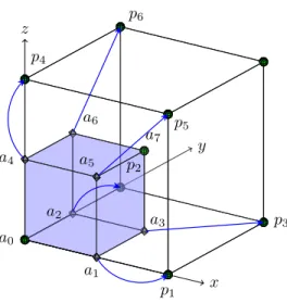
An octant with no children is called a “leaf” and an octant with one or more children is called an “interior octant”. “Complete” octrees are octrees in which every interior octant has exactly eight children. The only octant with no parent is the “root” and all other octants have exactly one parent. Octants that have the same parent are called “siblings”. The depth of an octant from the root is referred to as its “level”.8 We use a “linear” octree representation (i.e., we exclude interior octants) using the “Morton encoding” scheme [11, 18, 50, 51, 54, 56]. Any octant in the domain can be uniquely identified by specifying one of its vertices, also known as its “anchor”, and its level in the tree. By convention, the anchor of an octant is its front lower left corner (a0 in Figure 3.1). An octant’s configuration with respect to its parent
is specified by its “child number”: The octant’s position relative to its siblings in a sorted list. The child number of an octant is a function of the coordinates of its anchor and its level in the tree. For convenience, we use the Morton ordering to number the vertices of an octant. Hence, an octant with a child number equal to k will share its k-th vertex with its parent. This is a useful property that will be used frequently in the remaining sections. In order to perform finite element calculations of octrees, we impose a restriction on the relative sizes of adjacent octants. This is known as the “2:1 balance constraint” (not to be confused with load balancing): No octant should be more than twice the size of any other octant that shares a corner, edge or face with this octant. In the present work, we only work with complete, linear, 2:1 balanced octrees. In this paper, we use the balancing algorithm described in [51]. In this work, we only deal with sorted, complete, linear, 2:1 balanced octrees.
3.2. Finite elements on octrees. In our previous works [51,50], we developed low-cost algorithms and efficient data structures for constructing conforming finite element meshes using linear octrees. We use these data structures in the present work too. The key features of this framework are listed below.
• Given a complete linear 2:1 balanced octree, we use the leaves of the octree as the elements of a finite element mesh.
• A characteristic feature of such octree meshes is that they contain “hanging” vertices; these are vertices of octants that coincide with the centers of faces or mid-points of edges of other octants. The vertices of the former type are called “face-hanging” vertices and those of the latter type are called “edge-hanging” vertices. The 2:1 balance constraint ensures that there is at most one hanging vertex on any edge or face.
• We do not store hanging vertices explicitly. They do not represent indepen-dent degrees of freedom in a FEM solution.
• Since we handle hanging vertices in the meshing stage itself, we don’t need to use projection schemes like those used in [3,33,35,57] to enforce conformity. Hence, we don’t need multiple tree traversals for performing each MatVec; instead, we perform a single traversal by mapping each octant/element to one of the pre-computed element types, depending on the configuration of hanging vertices for that element.
• To reduce the memory overhead, the linear octree is stored in a compressed
6Sometimes, we use quadtrees for illustration purposes. Quadtrees are 2-D analogues of octrees. 7The term “node” is usually used to refer to the vertices of elements in a finite element mesh; but, in the context of tree data structures, it refers to the octants themselves.
z x y p1 p4 p2 p3 p5 p6 a4 a5 a7 a6 a0 a1 a2 a 3
Fig. 3.1.Illustration of nodal-connectivities required to perform conforming FEM calculations using a single tree traversal. Every octant has at least 2 non-hanging vertices, one of which is shared with the parent and the other is shared amongst all the siblings. The octant shown in blue (a)is a child 0, since it shares its zero vertex(a0)with its parent(p). It shares vertexa7 with its siblings. All other vertices, if hanging, point to the corresponding vertex of the parent octant instead. Vertices,a3, a5, a6are face hanging vertices and point top3, p5, p6, respectively. Similarlya1, a2, a4 are edge hanging vertices and point top1, p2, p4. All the vertices in this illustration are labelled in the Morton ordering.
form that requires only one byte per octant (the level of the octant). Even the element-to-vertex mappings can be compressed at a modest expense of uncompressing this on the fly while looping over the elements to perform the finite element MatVecs.
Below, we list some of the properties of the shape functions defined on octree meshes.
• The shape functions are not rooted at the hanging vertices.
• The shape functions are trilinear.
• The shape functions assume a value of 1 at the vertex at which they are rooted and a value of 0 at all other non-hanging vertices in the octree.
• The support of a shape function can spread over more than 8 elements.
• If a vertex of an element is hanging, then the shape functions rooted at the other non-hanging vertices in that element do not vanish on this hanging vertex. Instead, they will vanish at the non-hanging vertex that this hanging vertex is mapped to. If the i-th vertex of an element/octant is hanging, then the index corresponding to this vertex will point to the i-th vertex of the parent9 of this element instead. For example, in Figure 3.1 the shape function rooted at vertexa0 will not vanish at verticesa1,a2, a3,a4, a5 or
a6. It will vanish at vertices p1, p2, p3, p4, p5, p6 and a7. It will assume a
value equal to 1 at vertexa0.
• A shape function assumes non-zero values within an octant if and only if it is rooted at some non-hanging vertex of this octant or if some vertex of the octant under consideration is hanging, say the i-th vertex, and the shape
function in question is rooted at the i-th non-hanging vertex of the parent of this octant. Hence, for any octant there are exactly eight shape functions that do not vanish within it and their indices will be stored in the vertices of this octant.
• The finite element matrices constructed using these shape functions are math-ematically equivalent to those obtained using projection schemes such as in [35,56,57].
To implement finite element MatVecs using these shape functions, we need to enumerate all the permissible hanging configurations for an octant. The following properties of 2:1 balanced linear octrees helps reduce the total number of permissible hanging configurations. Figure3.1illustrates these properties.
• Every octant has at least 2 non-hanging vertices and they are: – The vertex that is common to both this octant and its parent. – The vertex that is common to this octant and all its siblings.
• An octant can have a face hanging vertex only if the remaining vertices on that face are one of the following:
– Edge hanging vertices.
– The vertex that is common to both this octant and its parent.
Any element in the mesh belongs to one of 8 child number based configurations. After factoring in the above constraints, there are only 18 potential hanging-vertex configurations for each child number configuration.
3.2.1. Overlapping communication with computation. Every octant is owned by a single processor. However, the values of unknowns associated with oc-tants on inter-processor boundaries need to be shared among several processors. We keep multiple copies of the information related to these octants and we term them “ghost” octants. In our implementation of the finite element MatVec, each processor iterates over all the octants it owns and also loops over a layer of ghost octants that contribute to the vertices it owns. Within the loops, each octant is mapped to one of the above described hanging configurations. This is used to select the appropriate element stencil from a list of pre-computed stencils. Although a processor needs to read ghost values from other processors it only needs to write data back to the ver-tices it owns and does not need to write to ghost verver-tices.10 Thus, there is only one
communication phase within each MatVec, which we can overlap with a computation phase:
1. Initiate non-blocking MPI sends for information stored on ghost-vertices. 2. Loop over the elements in the interior of the processor domain. These
el-ements do not share any vertices with other processors. We identify these elements during the meshing phase itself.
3. Receive ghost information from other processors. 4. Loop over remaining elements to update information.
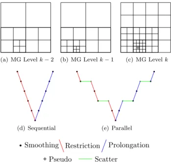
3.3. Global coarsening. Starting with the finest octree, we iteratively con-struct a hierarchy of complete, balanced, linear octrees such that every octant in the
k-th octree is either present in thek+ 1-th octree as well or all its eight children are present instead (Figures3.2(a) -3.2(c)).
We construct thek-th octree from the k+ 1-th octree by replacing every set of
10This is only possible because, our meshing scheme also builds the element-to-node connectivity mappings for the appropriate ghost elements. Although, this adds an additional layer of complexity to our meshing algorithm, it saves us one communication per MatVec.
eight siblings by their parent. This algorithm is based on the fact that in a sorted linear octree, each of the 7 successive elements following a “Child-0” element is either one of its siblings or a decendant of its siblings. Letiandjbe the indices of any two successive Child-0 elements in thek+ 1-th octree. We have the following 3 cases: (a)
j <(i+ 8), (b) j = (i+ 8) and (c)j >(i+ 8). In the first case, the elements with indices in the range [i, j) are not coarsened. In the second case, the elements with indices in the range [i, j) are all siblings of each other and are replaced by their parent. In the last case, the elements with indices in the range [i,(i+ 7)] are all siblings of each other and are replaced by their parent. The elements with indices in the range [(i+ 8), j) are not coarsened.
Coarsening is an operation withO(N) work complexity, whereN is the number of leaves in thek+ 1-th octree. It is easy to parallelize and has anO(N
np) parallel time
complexity, wherenp is the number of processors.11 The main parallel operations are two circular shifts; one clockwise and another anti-clockwise. The message in each case is just 1 integer: (a) the index of the first Child-0 element on each processor and (b) the number of elements between the last Child-0 element on any processor and the last element on that processor. While we communicate these messages in the background, we simultaneously process the elements in between the first and last Child-0 elements on each processor.
However, the operation described above may produce 4:1 balanced octrees12 in-stead of 2:1 balanced octrees. Hence, we balance the result using the algorithm described in [51]. This balancing algorithm has anO(NlogN) work complexity and
O(N nplog
N
np+nplognp) parallel time complexity. Although there is only one level of
imbalance that we need to correct, the imbalance can still affect octants that are not in its immediate vicinity. This is known as the “ripple effect”. Even with just one level of imbalance, a ripple can still propagate across many processors.
The sequence of octrees constructed as described above has the property that non-hanging vertices in any octree remain non-hanging in all the finer octrees as well. Hanging vertices on any octree could either become non-hanging on a finer octree or remain hanging on the finer octrees too. In addition, an octree can have new hanging as well as non-hanging vertices that are not present in any of the coarser octrees.
3.4. Intergrid transfer operations. To implement the intergrid transfer op-erations in Algorithm 1, we need to find all the non-hanging fine-grid vertices that lie within the support of each coarse-grid shape function. This is trivial on regular grids. However, for unstructured grids this can be quite expensive; especially for par-allel implementations. Fortunately, for a hierarchy of octree meshes constructed as described in Section3.3, these operations can be implemented quite efficiently.
As seen in Section 2.5, the restriction matrix is the transpose of the prolonga-tion matrix. We do not construct these matrices explicity, instead we implement a matrix-free scheme using MatVecs. The MatVecs for the restriction and prolongation operators are very similar. In both cases, we loop over the coarse and fine grid octants simultaneously. For each coarse-grid octant, the underlying fine-grid octant could ei-ther be the same as itself or be one of its eight children (Section3.3). We identify these cases and handle them separately. The main operation within the loop is selecting the coarse-grid shape functions that do not vanish within the current coarse-grid octant
11When we discuss communication costs we assume a Hypercube network topology withθ(n p) bandwidth.
12The input is 2:1 balanced and we coarsen by at most one level in this operation. Hence, this operation will only introduce one additional level of imbalance resulting in 4:1 balanced octrees.
(a) MG Levelk−2 (b) MG Levelk−1 (c) MG Levelk
(d) Sequential (e) Parallel
Smoothing Restriction Prolongation Pseudo Scatter
Fig. 3.2. (a)-(c)Quadtree meshes for three succesive multigrid levels.(d)A V-cycle where the meshes at all multigrid levels share the same partition and(e)A V-cycle where not all meshes share the same partition. Some meshes do share the same partition and whenever the partition changes a pseudo mesh is added. The pseudo mesh is only used to support intergrid transfer operations and smoothing is not performed on this mesh.
(Section3.2) and evaluating them at the non-hanging fine-grid vertices that lie within this coarse-grid octant. These form the entries of the restriction and prolongation matrices (Equation2.10).
To parallelize this operation, we need the coarse and fine grid partitions to be “aligned”. By aligned we require the following two conditions to be satisfied:
• If an octant exists both in the coarse and fine grids, then the same processor must “own” this octant on both the meshes.
• If an octant’s children exist in the fine-grid, then the same processor must own this octant on the coarse mesh and all its 8 children on the fine mesh. In order to satisfy these conditions, we first compute the partition on the coarse-grid and then impose it on the finer grid. In general, it might not be possible or desirable to use the same partition for all the multigrid levels. For example, the coarser multigrid levels might be too sparse to be distributed across all the processors or using the same partition for all the multigrid levels could lead to a large load imbalance across the processors. Hence, we allow some multigrid levels to be partitioned differently than others.13 When a transition in the partitions is required, we duplicate the
octree in question and let one of the duplicates share the same partition as that of its immediate finer multigrid level and let the other one share the same partition as that of its immediate coarser multigrid level. We refer to one of these duplicates as the “pseudo” mesh (Figure 3.2(e)). The pseudo mesh is only used to support intergrid transfer operations (Smoothing is not performed on this mesh). On these
13It is also possible that some processors are idle on the coarse-grids, while no processor is idle on the finer grids.
multigrid levels, the intergrid transfer operations include an additional step referred to as “Scatter”, which just involves re-distributing the values from one partition to another. One of the challenges with the MatVec for the intergrid transfer operations is that as we loop over the octants we must keep track of the pairs of coarse and fine grid vertices that were visited already. In order to implement this MatVec efficiently, we make use of the following observations.
• Every non-hanging fine-grid vertex is shared by at most eight fine-grid el-ements, excluding the elements whose hanging vertices are mapped to this vertex.
• Each of these eight fine-grid elements will be visited only once within the Restriction and Prolongation MatVecs.
• Since we loop over the coarse and fine elements simultaneously, there is a coarse octant associated with each of these eight fine octants. These coarse octants (maximum of eight) overlap with the respective fine octants.
• The only coarse-grid shape functions that do not vanish at the non-hanging fine-grid vertex under consideration are those whose indices are stored in the vertices of each of these coarse octants. Some of these vertices may be hanging, but they will be mapped to the corresponding non-hanging vertex. So, the correct index is always stored immaterial of the hanging state of the vertex.
We pre-compute and store a mask for each fine-grid vertex. Each of these masks is a set of eight bytes, one for each of the eight fine-grid elements that surround this fine-grid vertex. When we visit a fine-grid octant and the corresponding coarse-grid octant within the loop, we read the eight bits corresponding to this fine-grid octant. Each of these bits is a flag to determine whether or not the respective coarse-grid shape function contributes to this fine-grid vertex. The overhead of using this mask within the actual MatVecs includes(a)the cost of a few bitwise operations for each fine-grid octant and(b)the memory bandwidth required for reading the eight-byte mask. The latter cost is comparable to the cost required for reading a material property array within the finite element MatVec (for a variable coefficient operator). The restriction and prolongation MatVecs are operations with O(N) work complexity and have an
O(nN
p) parallel time complexity. The following section describes how we compute
these masks for any given pair of coarse and fine octrees.
3.4.1. Computing the “masks” for restriction and prolongation. Each non-hanging fine-grid vertex has a maximum14 of 1758 unique locations at which a coarse-grid shape function that contributes to this fine vertex could be rooted. Each of the vertices of the coarse-grid octants that overlap with the fine-grid octants surrounding this fine-grid vertex, can be mapped to one of these 1758 possibilities. It is also possible that some of these vertices are mapped to the same location. When we pre-compute the masks described earlier, we want to identify these many-to-one mappings and only one of them is selected to contribute to the fine-grid vertex under consideration.
Now, we briefly describe how we identified these 1758 cases. We first choose one of the eight fine-grid octants surrounding a given fine-grid vertex as a reference element. Without loss of generality, we pick the octant whose anchor is located at the given fine vertex. Now the remaining fine-grid octants could either be the same size as the reference element, or be half the size or twice the size of the reference
element. This simply follows from the 2:1 balance constraint. Further, each of these eight fine-grid octants could either be the same as the overlapping coarse-grid octant or be any of its eight children. Moreover, each of these coarse-grid octants that overlap the fine-grid octants under consideration could belong to any of the 8 child number types, each of which could further be of any of the 18 hanging configurations. Taking all these possible combinations into account, we can locate all the possible non-hanging coarse-grid vertices around a fine-grid vertex. Note that the child numbers, the hanging vertex configurations, and relative sizes of the eight fine-grid octants described above are not mutually independent. Each choice of child number, hanging vertex configuration and size for one of the eight fine-grid octants imposes numerous constraints on the respective choices for the other elements. However, to list all these possible constraints would be a complicated excercise and it is unnecessary for our purposes. Instead, we simply assume that the choices for the eight elements under consideration are mutually independent. This computation can be done offline and results in a weak upper bound of 1758 unique non-hanging coarse-grid locations around any fine-grid vertex.
We can not pre-compute the masks offline since this depends on the coarse and fine octrees under consideration. To do this computation efficiently, we employ a “PreMatVec” before we actually begin solving the problem; this is only performed once for each multigrid level. In this PreMatVec, we use a set of 16 bytes per fine-grid vertex; 2 bytes for each of the eight fine-grid octants surrounding the vertex. In these 16 bits, we store the flags for each of the possibilites described above. These flags contain the following information.
• A flag to determine whether or not the coarse and fine grid octants are the same (1 bit).
• The child number of the current fine-grid octant (3 bits).
• The child number of the corresponding coarse-grid octant (3 bits).
• The hanging configuration of the corresponding coarse-grid octant (5 bits).
• The relative size of the current fine-grid octant with respect to the reference element (2 bits).
Using this information and some simple bitwise operations, we can compute and store the masks for each fine-grid vertex. The PreMatVec is an operation withO(N) work complexity and has anO(nN
p) parallel time complexity.
3.4.2. Overlapping communication with computation. Finally, we overlap computation with communication for ghost values even within the Restriction and Prolongation MatVecs. However, unlike the finite element MatVec the loop is split into three parts because we can not loop over ghost octants since these octants need not be aligned across grids. Hence, each processor loops only over the coarse and the underlying fine octants that it owns. As a result, we need to both read as well as write to ghost values within the MatVec. The steps involved are listed below:
1. Initiate non-blocking MPI sends for ghost-values from the input vector. 2. Loop over some of the coarse and fine grid elements that are present in the
interior of the processor domains. These elements do not share any vertices with other processors.
3. Recieve the ghost-values sent from other processors in step 1.
4. Loop over the coarse and fine grid elements that share at least one of its vertices with a different processor.
5. Initiate non-blocking MPI sends for ghost-values in the output vector. 6. Loop over the remaining coarse and fine grid elements that are present in the
interior of the processor domains. Note in step 2, we only iterated over some of these elements. In this step, we iterate over the remaining elements. 7. Recieve the ghost-values sent from other processors in step 5.
8. Add the values recieved in step 7 to the existing values in the output vector. 3.5. Handling variable-coefficient operators. One of the problems with ge-ometric multigrid methods is that their performance deteriorates with increasing con-trast in material properties [17, 20]. Section 2.5 shows that the direct coarse-grid discretization can be used instead of the Galerkin coarse-grid operator provided the same bilinear form,a(u, v), is used both on the coarse and fine multigrid levels. This poses no difficulty for constant coefficient problems. For variable-coefficient problems, this means that the coarser grid MatVecs must be performed by looping over the un-derlying finest grid elements, using the material property defined on each fine-grid element. This would make the coarse-grid MatVecs quite expensive. A cheaper alter-native would be to define the material properties for the coarser grid elements as the average of those for the underlying fine-grid elements. This process amounts to using a different bilinear form for each multigrid level and hence is a clear deviation from the theory. This is one reason why the convergence of the stand-alone multigrid solver deteriorates with increasing contrast in material properties. Coarsening across discon-tinuities also affects the coarse grid correction, even when the Galerkin condition is satisfied. Large contrasts in material properties also affect simple smoothers like the Jacobi smoother. The standard solution is to use multigrid as a preconditioner to the Conjugate Gradient (CG) method [53]. We have conducted numerical experiments that demonstrate this for the Poisson problem. The method works well for smooth coefficients but it is not robust in the presence of discontinuous coefficients.
3.6. Minimum grain size required for good scalability. For good scalabil-ity of our algorithms, the number of elements in the interior of the processor domains must be significantly greater than the number of elements on the inter-processor boundaries. This is because our communication costs are proportional to the number of elements on the inter-processor boundaries and by keeping the number of such ele-ments small we can keep our communication costs low. Here we attempt to estimate the minimum grain size necessary to ensure that the number of elements in the inte-rior of a processor is greater than those on its surface. In order to do this, we assume the octree to be a regular grid. Consider a cube which is divided intoN3equal parts.
There are (N−2)3 small cubes in the interior of the large cube and N3−(N−2)3
small cubes touching the internal surface of the large cube. In order for the number of cubes in the interior to be more than the number of cubes on the surface,N must be >= 10 . Hence, the minimum grain size per processor is estimated to be 1000 elements.
3.7. Summary. The sequence of steps involved in solving the problem defined in Section2.1.1is summarized below:
1. A “sufficiently” fine152:1 balanced complete linear octree is constructed using
the algorithms described in [51].
2. Starting with the finest octree, a sequence of 2:1 balanced coarse linear octrees is constructed using the global coarsening algorithm (Section3.3).
3. The maximum number of processors that can be used for each multigrid level without violating the minimum grain size criteria (Section3.6) is computed.
4. Starting with the coarsest octree, the octree at each multigrid level is meshed using the algorithm described in [50]. As long as the load imbalance across the processors is acceptable and as long as the number of processors used for the coarser grid is the same as the maximum number of processors that can be used for the finer grid without violating the minimum grain size criteria, the partition of the coarser grid is imposed on to the finer grid during meshing. If either of the above two conditions is violated then the octree for the finer grid is duplicated; One of them is meshed using the partition of the coarser grid and the other is meshed using a fresh partition. The process is repeated until the finest octree has been meshed.
5. A restriction PreMatVec (Section 3.4) is performed at each multigrid level (except the coarsest) and the masks that will be used in the actual restriction and prolongation MatVecs are computed and stored.
6. For the case of variable-coefficient operators, vectors that store the material properties at each multigrid level are created.
7. The discrete system of equations is then solved using the conjugate gradient algorithm preconditioned with the multigrid scheme.
4. Numerical experiments. In this section, we consider solving foruin Equa-tion 4.1 and u in Equations 4.2, 4.3, 4.4 and 4.5. Equation 4.1 represents a 3-dimensional, linear elastostatics (vector) problem with isotropic and homogeneous Lam´e moduli (µand λ) and homogeneous Dirichlet boundary conditions. Equations 4.2 through4.5 represent 3-dimensional, linear Poisson (scalar) problems with inho-mogeneous material properties and hoinho-mogeneous Neumann boundary conditions.
µ∆u+ (λ+µ)∇Div u=f in Ω u=0in∂Ω µ= 1; λ= 4; Ω = [0,1]3 (4.1) −∇ ·(∇u) +u=f in Ω ˆ n· ∇u= 0 in∂Ω
(x, y, z) = 1 + 106 cos2(2πx) + cos2(2πy) + cos2(2πz) (4.2)
(x, y, z) = 107 if 0.3≤x, y, z≤0.6 1.0 otherwise (4.3) (x, y, z) =
107 if the index of the octant
containing (x, y, z) is divisible by some given integerK
1.0 otherwise (4.4) (x, y, z) = 107 if (x, y, z)∈[0,0.5)×[0,0.5)×[0,0.5) ∪[0.5,1.0]×[0.5,1.0]×[0,0.5) ∪[0,0.5)×[0.5,1.0]×[0.5,1.0] ∪[0.5,1.0]×[0,0.5)×[0.5,1.0] 1.0 otherwise (4.5)
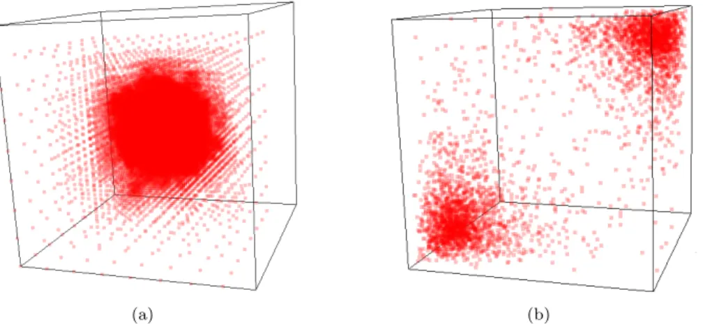
We discretized these problems on various octree meshes generated using Gaussian and log-normal distributions.16 Figures 4.1(a)and 4.1(b)respectively show samples of the Gaussian and log-normal distributions that were used in all our experiments.
(a) (b)
Fig. 4.1.Samples of the point distributions used for the numerical experiments:(a) A Guassian point distribution with mean at the center of the unit cube and(b) A log-normal point distribution with mean near one corner of the unit cube and it’s mirror image about the main diagonal.
The number of elements in these meshes range from about 25 thousand to over 1 billion and were solved on up to 12288 processors on the Teragrid systems: “Abe” (9.2K Intel-Woodcrest cores with Infiniband), “Bigben” (4.1K AMD Opteron cores with quadrics) and “Ranger” (63K Barcelona cores with Infiniband). Details for these systems can be found in [40,44,52]. Our C++ implementation uses MPI, PETSc [7] and SuperLU Dist [37]. The runs were profiled using PETSc.
In this section, we present the results from 5 sets of experiments: (A)A conver-gence test,(B)A robustness test,(C)Isogranular scalability,(D)Fixed size scalability and (E)Comparison with an off-the-shelf algebraic multigrid implementation. The parameters used in the experiments are listed below:
• For experiment (A), we setu= cos(2πx) cos(2πy) cos(2πz) and constructed the corresponding force (f).
• For experiments(B)through(E), we used a random solution (u) to construct the force (f).
• A zero initial guess was used in all experiments.
• One multigrid V-cycle was used as a preconditioner to the Conjugate Gradient (CG) method in all experiments. This is known to be more robust than the stand alone multigrid algorithm for variable-coefficient problems [53].
• The damped Jacobi method was used as the smoother at each multigrid level.
• SuperLU Dist [37] was used to solve the coarsest grid problem in all cases.
• In order to minimize communication costs, the coarsest grid used fewer pro-cessors than the finer grids. This keeps the setup cost for SuperLU Dist low. 4.1. Convergence Test. In the first experiment, a base discretization of ap-proximately ≈ 0.25M elements generated using the Gaussian distribution was used to solve the variable-coefficient problem (Equation 4.2). We measured the L2 norm
of the error as a function of the maximum element size (hmax) by uniformly refining the coarse elements17 in this base mesh. In Table4.1, we report the L2 norm of the
properties. In [47], we give some examples for constructing octrees based on user-supplied data such as material properties and source terms.
17Any element whose length is greater thanh max.
Max. Element Size (hmax) 1/16 1/32 1/64 1/128 1/256
L2norm of the error 3.98×10⁻³ 9.62×10⁻⁴ 2.46×10⁻⁴ 6.18×10⁻⁵ 1.56×10⁻⁵ Table 4.1
L2 norm of the error between the true solution and its finite element approximation for the variable coefficient problem (Equation4.2). The sequence of meshes used in this experiment were constructed by using a base discretization of ≈0.25M elements generated using a gaussian point distribution followed by successive uniform refinements of the coarse elements of this mesh.
log2K 1 4 7 10 13 16 19
Its. 119 18 25 55 66 43 17 Table 4.2
The number of iterations required to reduce the 2-norm of the residual in Equation4.4by a factor of10−8 for different values ofK, a parameter that controls the frequency of jumps. A regular grid with 128 elements in each dimension was used for this experiment.
error between the true solution and its finite element approximation for the sequence of meshes constructed as described above. A second order convergence is observed just as predicted by the theory.
4.2. Robustness Test. In the second experiment, we tested the robustness of the multigrid solver in the presence of strong jumps in the material properties. We discretized Equations4.4and4.5on an uniform octree with about 2M elements and measured the convergence rate for different values ofK. This octree is also a regular grid with 128 elements in each dimension. 6 Multigrid levels were used for these problems. In Table 4.2, we report the number of iterations that were required to reduce the 2-norm of the residual in Equation 4.4 by a factor of 10−8 for different
values of K; the number of jumps decreases as K increases. It is apparent that the solver is quite sensitive to the number of jumps. However, there are other factors that determine the overall performance of the solver. For example, it only takes 7 iterations to solve Equation4.5to the same tolerance; although there are more number of jumps in Equation 4.5than Equation 4.4for log2K = 10,13,16 or 19. While the fine grid
material properties in Equation 4.5 are represented exactly on all coarser grids, the fine grid material properties in Equation 4.4 are not represented accurately on any of the coarse grids. This would explain why coarse grid correction works better for Equation 4.5 than for Equation 4.4. The results of this experiment show that the current scheme is not robust in the presence of discontinuous coefficients.
4.3. Scalability Results. We tested the scalability of our implementation on the TeraGrid systems; all the fixed size (strong) scalability experiments were per-formed on Bigben and the iso-granular (weak) scalability experiments were perper-formed on both Bigben and Ranger. In all the fixed-size and iso-granular scalability results, the reported times for each component are the maximum values for that component across all the processors. Hence, in some cases the total time18 is lower than the sum of the individual components. We also report the theoretical predictions19 for the total setup and solve times. This was computed using the asymptotic complexity estimates for the setup (O(N
nplog
N
np) +O(nplognp)) and solve (O(
N
np) +O(lognp))
times. The coefficients in the expressions for the complexity were computed so that the sum of squares of the deviation between the theoretical estimates and the actual data is minimized. While determining these coefficients, we skipped the last data
18This is reported in bold face.
point (corresponding to the greatest number of processors) in each experiment. This was done so that we could use our model to predict the value for the last data point and compare our predictions with the observed results. The number of multigrid lev-els and the total number of meshes generated for each case is also reported. Note that due to the addition of auxillary meshes, the total number of meshes is greater than the number of multigrid levels. The setup cost includes the time for constructing the mesh for all the multigrid levels (including the finest), constructing and balancing all the coarser multigrid levels and setting up the intergrid transfer operators by per-forming one PreMatVec at each multigrid level. The time to create the work vectors for the MG scheme and the time to build the coarsest grid matrix are also included in the total setup time, but are not reported individually since they are insignificant. “Scatter” refers to the process of transferring the vectors between two different par-titions of the same multigrid level during the intergrid transfer operations, required whenever the coarse and fine grids do not share the same partition. The time spent in applying the Jacobi preconditioner, computing the inner-products within CG and solving the coarsest grid problems using LU are all accounted for in the total solve time, but are not reported individually since they are insignificant. When we report
MPI Wait()times, we refer to synchronization for non-blocking operations during the Restriction, Prolongation and Finite Element MatVecs.
4.3.1. Isogranular (Weak) scalability. Isogranular scalability analysis was performed by tracking the execution time while increasing the problem size and the number of processors proportionately. The results from isogranular scalability ex-periments on the octrees generated from Gaussian point distributions are reported in Tables4.3,4.4and4.5. Tables4.3and4.4report the results for the constant coefficient elasticity (Equation 4.1) problem for two different grain sizes and Table4.5 reports the results for the variable-coefficient Poisson problem (Equation 4.2). The results from an isogranular scalability experiment for solving the variable-coefficient Poisson problem (Equation4.2) on octrees generated from log-normal point distributions are reported in Table4.6. There is little variation between the Gaussian distribution case and the log-normal distribution case. For the Gaussian distribution cases, the coarsest octant at the finest multigrid level was at level 3; the level of the finest octant at the finest multigrid level for each case is reported in the tables. The octrees considered here are extremely non-uniform–roughly five-orders of magnitude variation in the leaf size. It is also quite promising that the setup costs are smaller than the solution costs, suggesting that the method is suitable for problems that require the construction and solution of linear systems of equations numerous times. The increase in running times for the large processor cases can be primarily attributed to poor load balancing. This is evident from(a)the imbalance in the number of elements per processor and (b)
the time spent in calls toMPI Wait(). These numbers are reported in Tables4.3and 4.4.20 Load balancing is a challenging problem due to the following reasons:
• We need to make an accurate a-priori estimate of the computation and com-munication loads. It is difficult to make such estimates for arbitrary distri-butions.
• For the intergrid transfer operations, the coarse and fine grids need to be aligned. It is difficult to get good load balance for both the grids, especially for non-uniform distributions.
20We only report the Max/Min elements ratios for the finest multigrid level although the trend is similar for other multigrid levels as well.
CPUs Coarsening Balancing Meshing R-setup Total Setup (Theory) LU R + P Scatter FE Matvecs Total Solve (Theory) Meshes MG Levels Elements Max/Min Elements
MPI Wait (sec) Finest Octant’s Level 12 0.33 0.77 0.9725 0.092 2.41 (2.8) 0.189 2.53 3.11 51.63 54.82 (55.57) 11 8 337.8K 1.89 21.32 12 48 0.56 0.99 1.44 0.125 3.22 (2.9) 0.4 3.62 6.49 57.73 63.74 (61.66) 16 11 1.34M 1.79 24.32 15 192 0.95 1.23 1.82 0.122 3.87 (3.52) 0.017 4.23 8.59 60.20 66.14 (67.55) 19 12 5.29M 2.04 29.58 16 768 1.66 1.84 3.32 0.14 6.51 (6.94) 0.171 5.36 13.13 64.58 73.5 (73.99) 24 14 21.15M 2.82 32.65 18 3072 2.18 4.48 15.09 0.172 23.4 (23.33) 0.543 8.55 16.98 68.78 80.96 (80.40) 25 14 84.5M 3.9 39.8 18 12288 4.39 12.66 32.89 0.173 53.21 (99.59) 0.015 8.96 21.15 69.87 85.28 (86.90) 28 15 338.3M 3.08 39.19 19 Table 4.3
Isogranular scalability for solving the constant coefficient linear elastostatics problem on a set of octrees with a grain size (on the finest multigrid level) of30K(approx)elements per CPU(np)
generated using a Gaussian distribution of points. A relative tolerance of 10−10 in the 2-norm of the residual was used. 11 iterations were required in each case, to solve the problem to the specified tolerance. This experiment was performed on “Ranger”.
• Partitioning each multigrid level independently to get good load balance for the smoothing operations at each multigrid level would require the creation of an auxillary mesh for each multigrid level and a scatter operation for each intergrid transfer operation at each multigrid level. This would increase the setup costs and the communication costs.
4.3.2. Fixed-size (Strong) scalability. Fixed-size scalability was performed on the octrees generated from Gaussian and log-normal point distributions to compute the speedup when the problem size is kept constant and the number of processors is increased. The results from fixed size scalability experiments for the solving the variable-coefficient problem (Equation4.2) on an octree with 32M (approx) elements generated from Gaussian point distribution are reported in Table4.7. This experiment was repeated on octrees with 6M and 22M (approx) elements generated from log-normal point distributions and the corresponding results are reported in Tables4.9and 4.8, respectively. The results for the Gaussian and log-normal distributions are similar. We observe nearly ideal speed-ups for the setup phase on up to 256 processors and the speed-ups begin to deteriorate beyond that. We believe that the surface computation (e.g. meshing for ghost elements) begins to dominate beyond 256 processors. Note that the number of meshes also grow with the number of processors. This is another
CPUs Coarsening Balancing Meshing R-setup Total Setup (Theory) LU R + P Scatter FE Matvecs Total Solve (Theory) Meshes MG Levels Elements Max/Min Elements
MPI Wait (sec) Finest Octant’s Level 12 0.85 1.76 2.41 0.27 4.64 (6.95) 0.025 6.22 3.9 145.8 152.36 (156.26) 13 10 986.97K 1.66 53.95 14 48 1.27 2.08 3.21 0.32 5.95 (7.15) 0.02 7.89 6.1 166.73 175.2 (170.15) 16 11 3.97M 1.9 80.23 15 192 2.18 2.96 6.53 0.323 11.04 (7.98) 0.517 12.87 13.83 174.27 187.27 (183.22) 22 12 15.87M 2.44 97.86 17 768 3.09 3.87 7.4 0.32 12.85 (12.16) 0.048 13.8 15.26 173.64 188.38 (196.20) 25 14 63.4M 2.43 88.1 18 3072 4.17 7.19 21.06 0.35 31.89 (32.15) 4.92 14.87 20.63 186.11 212.04 (209.45) 27 15 253.8M 2.73 97.83 19 12288 6.28 13.33 33.41 0.54 54.69 (125.1) 0.019 56.2 62.61 221.01 242.37 (221.92) 29 16 1.01B 2.88 173.82 20 Table 4.4
Isogranular scalability for solving the constant coefficient linear elastostatics problem on a set of octrees with a grain size (on the finest multigrid level) of80K(approx)elements per CPU(np)
generated using a Gaussian distribution of points. A relative tolerance of 10−10 in the 2-norm of the residual was used. 11 iterations were required in each case, to solve the problem to the specified tolerance. This experiment was performed on “Ranger”.
reason why we don’t observe ideal speed-ups for the setup phase. The speed-ups for the solve phase, although not ideal, seem to be quite good. Poor load balancing, which affects isogranular scalability on large processor counts, seems to be another factor that affects the speed-ups for the setup and solve phases in the fixed-size scalability experiments.
4.4. Comparison with BoomerAMG. Finally, the results from the compari-son between the geometric multigrid (GMG) and algebraic multigrid (BoomerAMG) schemes for the variable-coefficient problem (Equation4.3) are reported in Table4.10. This experiment was performed on Abe. Each node of the cluster has 8 processors, which share an 8GB RAM. However, only 1 processor per node was utilized in the above experiments. This is because the AMG scheme required a lot of memory and this allowed the entire memory on any node to be available for a single process. For BoomerAMG, we experimented with two different coarsening schemes: Falgout coars-ening and CLJP coarscoars-ening. The results from both experiments are reported. [32] reports that Falgout coarsening works best for structured grids and CLJP coarsening is better suited for unstructured grids. Since octree meshes lie in between both struc-tured and generic unstrucstruc-tured grids, we compare our results using both the schemes. While the convergence rate of the geometric multigrid method deteriorates with
in-CPUs Coarsening Balancing Meshing R-setup Total Setup (Theory) LU R + P Scatter FE Matvecs Total Solve (Theory) Elements Vertices Meshes MG Levels Finest Octant’s Level 1 0.047 0.57 5.01 0.946 6.72 (16.69) 0.54 2.86 0 55.36 58.71 (66.92) 239.4K 151.7K 4 4 8 4 0.145 3.41 10.93 1.95 16.62 (17.41) 0.116 14.72 0.124 96.33 101.76 (91.78) 995.4K 660.1K 7 7 14 16 0.146 7.0 10.95 1.66 20.04 (17.45) 0.566 21.21 0.228 97.24 102.67 (113.8) 3.97M 2.68M 8 7 14 64 0.147 7.51 12.13 1.75 22.0 (18.14) 3.43 25.81 0.49 121.0 134.34 (136.55) 16.0M 10.52M 9 7 16 256 0.182 8.38 14.06 2.04 26.13 (21.12) 4.23 41.31 2.15 184.4 195.45 (159.21) 64.4M 42.0M 11 8 18 1024 0.288 11.44 18.8 1.96 33.95 (35.11) 6.18 33.02 4.64 138.84 156.0 (181.21) 256.8M 172.4M 14 9 19 4096 1.51 15.58 36.82 2.11 60.9 (102.11) 9.8 54.07 9.64 249.36 274.71 (204.31) 1.04B 702.9M 16 10 21 Table 4.5
Isogranular scalability for solving the variable-coefficient Poisson problem (Equation 4.2) on the set of octrees with a grain size (on the finest multigrid level) of 0.25M elements (approx.) per processor(np) generated using a Gaussian distribution of points. The iterations were terminated
when the 2-norm of the residual was reduced by a factor of10−10. 5 iterations were required in each case. This experiment was performed on “Bigben”.
creasing contrast in the material properties, the convergence rate of BoomerAMG is not affected by contrasts in the material properties. Hence, the variable-coefficient problem is more interesting for this experiment. This experiment shows that GMG has a much lower setup cost compared to AMG; the solution costs are comparable. The AMG scheme seems to have a higher convergence rate since it takes fewer iterations as compared to GMG.
5. Conclusions. We have described a parallel geometric multigrid method for solving elliptic partial differential equations using finite elements on octree based discretizations. The features of the described method are summarized below:
• We automatically generate a sequence of coarse meshes from an arbitrary 2:1 balanced fine octree. We do not impose any restrictions on the number of meshes in this sequence or the size of the coarsest mesh. We do not require the meshes to be aligned and hence the different meshes can be partitioned independently to satisfy any user-defined constraint such as a limit on the load imbalance. Although, the process of constructing coarser meshes from a fine mesh is harder than iterative global refinements of a coarse mesh to generate a sequence of fine meshes; this is more practical since the fine mesh can be defined naturally depending on modeling restrictions, and/or physics of the problem as opposed to the coarse mesh, which is purely an artifact of the numerical method. It is also natural and more desirable to be able to
CPUs Coarsening Balancing Meshing R-setup Total Setup (Theory) LU R + P Scatter FE Matvecs Total Solve (Theory) CG Its. Meshes MG Levels Finest Octant’s Level Coarsest Octant’s Level Elements Vertices 1 0.005 0.059 0.565 0.098 0.85 (2.37) 0.102 0.315 0 6.56 7.05 (7.96) 5 3 3 9 3 24.6K 17.4K 4 0.013 0.319 1.32 0.162 1.89 (2.41) 0.178 1.47 0.061 10.9 11.81 (9.18) 5 5 4 13 3 99.3K 68.2K 16 0.013 0.67 1.87 0.158 2.89 (2.36) 0.276 1.2 0.52 6.33 7.48 (9.62) 5 8 5 13 4 362.6K 243.3K 64 0.016 0.99 3.83 0.151 5.43 (3.27) 0.098 1.62 1.88 8.57 9.98 (10.61) 6 13 7 13 4 1.42M 952.2K 256 0.042 1.26 5.75 0.165 7.86 (8.28) 0.177 1.13 3.75 10.16 12.58 (11.70) 5 15 8 15 5 5.64M 3.79M 1024 0.123 1.78 9.04 0.174 12.11 (33.0) 1.08 1.33 6.14 10.89 15.27 (12.79) 5 15 8 16 5 22.4M 14.9M Table 4.6
Isogranular scalability for solving the variable-coefficient Poisson problem (Equation4.2) on a set of octrees with a grain size (on the finest multigrid level) of 25K elements (approx.) per processor (np)generated using a log-normal distributions of points located on two diagonally opposite corners
of the unit cube. The iterations were terminated when the 2-norm of the residual was reduced by a factor of10−10. 5 iterations were required in each case. The levels of the coarsest and finest octants at the finest multigrid level are reported in the table. This experiment was performed on “Bigben”.
control the fine mesh in an adaptive algorithm rather than controlling the coarse mesh.
• We have demonstrated good scalability of our implementation and can solve problems with billions of elements on thousands of processors in less than 10 minutes. However, load balancing remains an open problem and this begins to affect our iso-granular scalability beyond a thousand processors. This is a difficult problem to tackle because there are many competing factors: Restriction, prologation, scatters and MatVecs.
• We have demonstrated that our implementation works well even on problems with variable coefficients.
• We have compared our geometric multigrid implementation with the alge-braic multigrid scheme (BoomerAMG) implemented in a standard off-the-shelf package (HYPRE) and show that the proposed algorithm is quite com-petent. The setup cost for the matrix-free geometric multigrid algorithm is much lower than its algebraic multigrid counterpart. This makes it better suited for problems in which the linear system of equations is constructed and
CPUs Coarsening Balancing Meshing R-setup Total Setup (Theory) LU R + P Scatter FE Matvecs Total Solve (Theory) Meshes 32 0.59 20.69 52.1 8.224 83.08 (84.65) 1.67 68.2 0.055 344.91 374.57 (405.57) 9 64 0.293 12.69 24.43 3.87 42.02 (40.77) 1.66 54.35 1.04 245.85 266.44 (219.69) 10 128 0.163 8.174 13.06 1.82 23.99 (20.64) 1.66 36.85 1.39 170.22 180.09 (129.17) 11 256 0.108 5.468 8.504 0.95 15.87 (12.76) 1.65 12.21 2.29 54.22 60.98 (86.32) 12 512 0.091 3.34 5.597 0.487 10.68 (12.76) 1.65 6.57 2.52 30.76 36.29 (67.31) 12 1024 0.133 2.76 5.927 0.243 10.31 (20.98) 1.64 2.83 4.17 14.34 19.36 (60.23) 14 Table 4.7
Fixed-size scalability for solving the variable-coefficient Poisson problem (Equation4.2) on an octree with 31.9M elements generated from a gaussian distribution of points. 8 Multigrid levels were used. 5 iterations were required to reduce the 2-norm of the residual by a factor of 10−10. 468 Matvecs, 72 of which are on the finest grid, were required.
CPUs Coarsening Balancing Meshing R-setup Total Setup (Theory) LU R + P Scatter FE Matvecs Total Solve (Theory) 32 0.41 14.37 59.19 4.4 79.85 (84.91) 1.1 70.16 27.95 334.1 352.14 (374.45) 64 0.21 8.44 35.81 2.26 47.55 (41.29) 1.11 44.38 21.38 236.7 246.43 (197.13) 128 0.12 5.63 22.06 1.14 29.96 (21.89) 1.1 7.86 19.63 92.08 103.4 (109.89) 256 0.083 3.11 15.36 0.58 20.14 (15.69) 1.1 5.29 17.43 62.33 71.22 (67.68) 512 0.084 2.19 11.93 0.33 15.53 (19.42) 1.1 2.56 10.42 22.99 29.42 (47.99) 1024 0.123 1.78 9.04 0.17 12.11 (35.82) 1.1 1.33 6.14 10.89 15.27 (39.56) Table 4.8
Fixed-size scalability for solving the variable-coefficient Poisson problem (Equation 4.2) on an octree with 22.4M elements generated using a log-normal distribution of points located on two diagonally opposite corners of the unit cube. 8 Multigrid levels and 15 meshes were used. 5 iterations were required to reduce the 2-norm of the residual by a factor of10−10.
solved numerous times. Examples of such problems include time-dependent problems, non-linear problems and applications with adaptive mesh refine-ment proceedures.
• Our MPI-based implementation, DENDRO, is built on top of PETSc [6, 7]. Dendro is an open source code that can be downloaded from [46].
CPUs Coarsening Balancing Meshing R-setup Total Setup (Theory) LU R + P Scatter FE Matvecs Total Solve (Theory) 32 0.11 5.1 16.89 1.17 23.95 (26.25) 0.18 16.89 8.18 87.91 92.83 (101.0) 64 0.057 2.99 11.21 0.56 15.42 (12.82) 0.18 11.62 5.2 65.55 69.92 (52.65) 128 0.043 1.96 8.24 0.34 11.33 (7.07) 0.18 2.18 19.98 26.76 30.21 (28.79) 256 0.042 1.26 5.75 0.16 7.86 (5.70) 0.18 1.13 3.75 10.16 12.58 (17.16) 512 0.064 0.99 4.3 0.11 6.09 (8.02) 0.18 0.84 3.51 6.09 7.64 (11.65) 1024 0.13 0.94 3.75 0.079 5.49 (15.61) 0.18 0.75 4.68 5.14 8.3 (9.21) Table 4.9
Fixed-size scalability for solving the variable-coefficient Poisson problem (Equation 4.2) on an octree with 5.64M elements generated using a log-normal distribution of points located on two diagonally opposite corners of the unit cube. 8 Multigrid levels and 15 meshes were used. 5 iterations were required to reduce the 2-norm of the residual by a factor of10−10.
There are two important extensions for the present work: higher-order discretizations and integration with domain-decomposition methods such as the Heirarchical Hybrid Grids (HHG) scheme described in [10]. The former will result in improved accuracy with fewer elements and the latter will help solve problems involving complicated geometries with fewer elements. The last point stems from the fact that using a single octree to mesh a domain is more restrictive than allowing the use of multiple octrees, each of which is only responsible for a part of the entire domain.
Acknowledgments. This work was supported by the U.S. Department of En-ergy under grant DE-FG02-04ER25646 and the U.S. National Science Foundation under grants CCF-0427985, CNS-0540372, DMS-0612578, 0749285 and OCI-0749334. Computing resources on the TeraGrid systems were provided under the grants ASC070050N and MCA04T026. We also thank the TeraGrid support staff and consultants at NCSA, PSC and TACC.
REFERENCES
[1] M. F. Adams, H.H. Bayraktar, T.M. Keaveny, and P. Papadopoulos. Ultrascalable implicit finite element analyses in solid mechanics with over a half a billion degrees of freedom. In Proceedings of SC2004, The SCxy Conference series in high performance networking and computing, Pittsburgh, Pennsylvania, 2004. ACM/IEEE.
[2] Mark Adams and James W. Demmel. Parallel multigrid solver for 3d unstructured finite element problems. InSupercomputing ’99: Proceedings of the 1999 ACM/IEEE conference on Supercomputing (CDROM), page 27, New York, NY, USA, 1999. ACM Press.
[3] Volkan Akcelik, Jacobo Bielak, George Biros, Ioannis Epanomeritakis, Antonio Fernandez, Omar Ghattas, Eui Joong Kim, Julio Lopez, David R. O’Hallaron, Tiankai Tu, and John Urbanic. High resolution forward and inverse earthquake modeling on terascale comput-ers. InSC ’03: Proceedings of the 2003 ACM/IEEE conference on Supercomputing. ACM, 2003.
CPUs GMG Setup GMG Solve Falgout Setup Falgout Solve CLJP Setup CLJP Solve Elements 1 1.21 9.23 7.86 5.54 6.09 2.56 52K 2 2.42 16.6 18.97 11.77 14.12 6.11 138K 4 2.11 14.19 18.9 7.23 13.41 3.96 240K 8 2.05 14.76 30 9.25 20.08 4.77 0.5M 16 5.19 21.07 41.56 11.35 24.77 6.38 995K 32 5.67 22.49 59.29 13.91 34.54 6.92 2M 64 6.63 19.2 92.61 14.5 52.05 8.12 3.97M 128 6.84 20.33 146.23 18.56 80.09 9.4 8M 256 10.7 22.23 248.5 23.3 151.64 13.9 16M Table 4.10
The variable-coefficient (contrast of107) Poisson problem (Equation4.3) was solved on meshes constructed on Gaussian distributions. A 7-level multiplicative-multigrid cycle was used as a pre-conditioner to CG for the GMG scheme. The coarsest grid was distributed on a maximum of 32 processors. For BoomerAMG, we experimented with two different coarsening schemes: Falgout coarsening and CLJP coarsening. Both GMG and AMG schemes used 4 pre-smoothing steps and 4 post-smoothing steps per multigrid level with the damped Jacobi smoother. A relative tolerance of 10−10 in the 2-norm of the residual was used in all the experime