TOPICAL REVIEW
Electrowetting: from basics to applications
Frieder Mugele1,3and Jean-Christophe Baret1,2
1University of Twente, Faculty of Science and Technology, Physics of Complex Fluids, PO Box
217, 7500 AE Enschede, The Netherlands
2Philips Research Laboratories Eindhoven, Health Care Devices and Instrumentation, WAG01,
Prof. Holstlaan 4, 5656 AA Eindhoven, The Netherlands E-mail:[email protected]
Received 11 April 2005, in final form 10 May 2005 Published 1 July 2005
Online atstacks.iop.org/JPhysCM/17/R705
Abstract
Electrowetting has become one of the most widely used tools for manipulating tiny amounts of liquids on surfaces. Applications range from ‘lab-on-a-chip’ devices to adjustable lenses and new kinds of electronic displays. In the present article, we review the recent progress in this rapidly growing field including both fundamental and applied aspects. We compare the various approaches used to derive the basic electrowetting equation, which has been shown to be very reliable as long as the applied voltage is not too high. We discuss in detail the origin of the electrostatic forces that induce both contact angle reduction and the motion of entire droplets. We examine the limitations of the electrowetting equation and present a variety of recent extensions to the theory that account for distortions of the liquid surface due to local electric fields, for the finite penetration depth of electric fields into the liquid, as well as for finite conductivity effects in the presence of AC voltage. The most prominent failure of the electrowetting equation, namely the saturation of the contact angle at high voltage, is discussed in a separate section. Recent work in this direction indicates that a variety of distinct physical effects—rather than a unique one— are responsible for the saturation phenomenon, depending on experimental details. In the presence of suitable electrode patterns or topographic structures on the substrate surface, variations of the contact angle can give rise not only to continuous changes of the droplet shape, but also to discontinuous morphological transitions between distinct liquid morphologies. The dynamics of electrowetting are discussed briefly. Finally, we give an overview of recent work aimed at commercial applications, in particular in the fields of adjustable lenses, display technology, fibre optics, and biotechnology-related microfluidic devices.
(Some figures in this article are in colour only in the electronic version) 3 Author to whom any correspondence should be addressed.
Contents
1. Introduction 706
2. Theoretical background 708
2.1. Basic aspects of wetting 708 2.2. Electrowetting theory for homogeneous substrates 710 2.3. Extensions of the classical electrowetting theory 715
3. Materials properties 719
4. Contact angle saturation 722 5. Complex surfaces and droplet morphologies 725 5.1. Morphological transitions on structured surfaces 725 5.2. Patterned electrodes 726 5.3. Topographically patterned surfaces 727 5.4. Self-excited oscillatory morphological transitions 730 5.5. Electrostatic stabilization of complex morphologies 731 5.6. Competitive wetting of two immiscible liquids 732 6. Dynamic aspects of electrowetting 732
7. Applications 734
7.1. Lab-on-a-chip 734
7.2. Optical applications 737 7.3. Miscellaneous applications 741 8. Conclusions and outlook 741
Acknowledgments 742
Appendix A. Relationships between electrical and capillary phenomena 743
A.1. First law 744
A.2. Second law 749
A.3. Mathematical theory 754 A.4. Electrocapillary motor 757 A.5. Measurement of the capillary constant of mercury in a conducting liquid 760 A.6. Capillary electrometer 762 A.7. Theory of the whirls discovered by Gerboin 766
References 770
1. Introduction
Miniaturization has been a technological trend for several decades. What started out initially in the microelectronics industry long ago reached the area of mechanical engineering, including fluid mechanics. Reducing size has been shown to allow for integration and automation of many processes on a single device giving rise to a tremendous performance increase, e.g. in terms of precision, throughput, and functionality. One prominent example from the area of fluid mechanics the ‘lab-on-a-chip’ systems for applications such as DNA and protein analysis, and biomedical diagnostics [1–3]. Most of the devices developed so far are based on continuous flow through closed channels that are either etched into hard solids such as silicon and glass, or replicated from a hard master into a soft polymeric matrix. Recently, devices based on the manipulation of individual droplets with volumes in the range of nanolitres or less have attracted increasing attention [4–10].
From a fundamental perspective the most important consequence of miniaturization is a tremendous increase in the surface-to-volume ratio, which makes the control of surfaces and surface energies one of the most important challenges both in microtechnology in general as
well as in microfluidics. For liquid droplets of submillimetre dimensions, capillary forces dominate [11,12]. The control of interfacial energies has therefore become an important strategy for manipulating droplets at surfaces [13–17]. Both liquid–vapour and solid–liquid interfaces have been influenced in order to control droplets, as recently reviewed by Darhuber and Troian [15]. Temperature gradients as well as gradients in the concentration of surfactants across droplets give rise to gradients in interfacial energies, mainly at the liquid–vapour interface, and thus produce forces that can propel droplets making use of the thermocapillary and Marangoni effects.
Chemical and topographical structuring of surfaces has received even more attention. Compared to local heating, both of these two approaches offer much finer control of the equilibrium morphology. The local wettability and the substrate topography together provide boundary conditions within which the droplets adjust their morphology to reach the most energetically favourable configuration. For complex surface patterns, however, this is not always possible as several metastable morphologies may exist. This can lead to rather abrupt changes in the droplet shape, so-called morphological transitions, when the liquid is forced to switch from one family of morphologies to another by varying a control parameter, such as the wettability or the liquid volume [13,16,18–20].
The main disadvantage of chemical and topographical patterns is their static nature, which prevents active control of the liquids. Considerable work has been devoted to the development of surfaces with controllable wettability—typically coated with self-assembled monolayers. Notwithstanding some progress, the degree of switchability, the switching speed, the long term reliability, and the compatibility with variable environments that have been achieved so far are not suitable for most practical applications. In contrast, electrowetting (EW) has proven very successful in all these respects: contact angle variations of several tens of degrees are routinely achieved. Switching speeds are limited (typically to several milliseconds) by the hydrodynamic response of the droplet rather than the actual switching of the equilibrium value of the contact angle. Hundreds of thousands of switching cycles were performed in long term stability tests without noticeable degradation [21,22]. Nowadays, droplets can be moved along freely programmable paths on surfaces; they can be split, merged, and mixed with a high degree of flexibility. Most of these results were achieved within the past five years by a steadily growing community of researchers in the field4.
Electrocapillarity, the basis of modern electrowetting, was first described in detail in 1875 by Gabriel Lippmann [23]. This ingenious physicist, who won the Nobel prize in 1908 for the discovery of the first colour photography method, found that the capillary depression of mercury in contact with electrolyte solutions could be varied by applying a voltage between the mercury and electrolyte. He not only formulated a theory of the electrocapillary effect but also developed several applications, including a very sensitive electrometer and a motor based on his observations. In order to make his fascinating work, which has only been available in French up to now, available to a broader readership, we included a translation of his work in the appendix of this review. The work of Lippmann and of those who followed him in the following more than a hundred years was devoted to aqueous electrolytes in direct contact with mercury surfaces or mercury droplets in contact with insulators. A major obstacle to broader applications was electrolytic decomposition of water upon applying voltages beyond a few hundred millivolts. The recent developments were initiated by Berge [24] in the early 1990s, who introduced the idea of using a thin insulating layer to separate the conductive liquid from the metallic electrode in order to eliminate the
4 The number of publications on electrowetting has been increasing from less than five per year before 2000 to 8 in
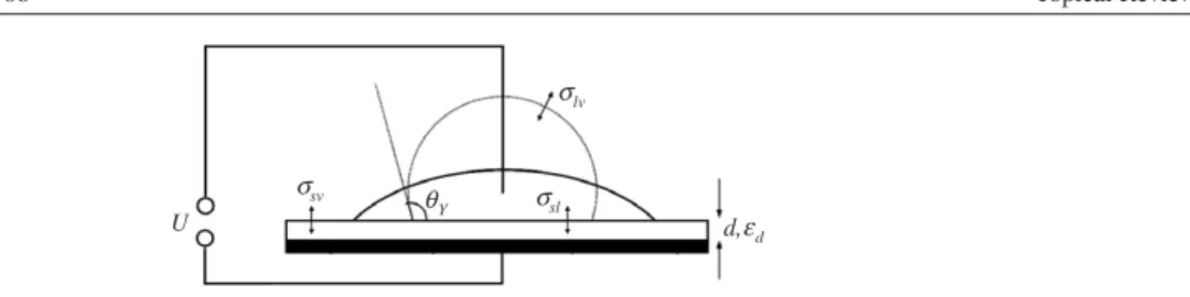
σlv εd σsl σsv θ Y U d,
Figure 1. Generic electrowetting set-up. Partially wetting liquid droplet at zero voltage (dashed) and at high voltage (solid). See the text for details.
problem of electrolysis. This is the concept that has also become known as electrowetting on dielectric (EWOD).
In the present review, we are going to give an overview of the recent developments in electrowetting, touching only briefly on some of the early activities that were already described in a short review by Quilliet and Berge [25]. The article is organized as follows. In section2 we discuss the theoretical background of electrowetting, comparing different fundamental approaches, and present some extensions of the classical models. Section 3 is devoted to materials issues. In section4, we discuss the phenomenon of contact angle saturation, which has probably been the most fundamental challenge in electrowetting for some time. Section5 is devoted to the fundamental principles of electrowetting on complex surfaces, which is the basis for most applications. Section6deals with some aspects of dynamic electrowetting, and finally, before concluding, a variety of current applications ranging from lab-on-a-chip to lens systems and display technology are presented in section7.
2. Theoretical background
Electrowetting has been studied by researchers from various fields, such as applied physics, physical chemistry, electrochemistry, and electrical engineering. Given the various backgrounds, different approaches were used to describe the electrowetting phenomenon, i.e. to determine the dependence of the contact angle on the applied voltage. In this section, we will— after a few introductory remarks about wetting in section2.1—discuss the main approaches of electrowetting theory (section2.2): the classical thermodynamic approach (2.2.1), the energy minimization approach (2.2.2), and the electromechanical approach (2.2.3). In section2.3, we will describe some extensions of the basic theories that give more insight into the microscopic surface profile near the three-phase contact line (2.3.1), the distribution of charge carriers near the interface (2.3.2), and the behaviour at finite frequencies (2.3.3).
2.1. Basic aspects of wetting
In electrowetting, one is generically dealing with droplets of partially wetting liquids on planar solid substrates (see figure1). In most applications of interest, the droplets are aqueous salt solutions with a typical size of the order of 1 mm or less. The ambient medium can be either air or another immiscible liquid, frequently an oil. Under these conditions, the Bond number Bo=gρR2/σlv, which measures the strength of gravity with respect to surface tension, is smaller than unity. Therefore we neglect gravity throughout the rest of this paper. In the absence of external electric fields, the behaviour of the droplets is then determined by surface tension alone. The free energyFof a droplet is a functional of the droplet shape. Its value is given by the sum of the areasAiof the interfaces between three phases, the solid substrate (s),
σlv
σsl σsv
θY
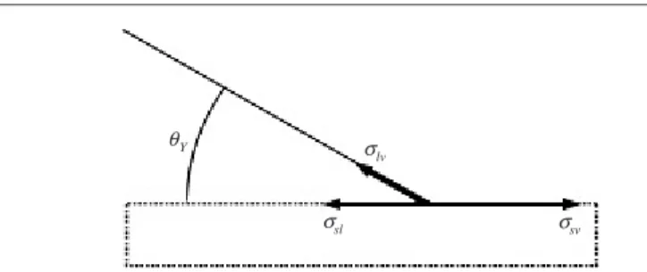
Figure 2. Force balance at the contact line (forθYapproximately 30◦).
the liquid droplet (l), and the ambient phase, which we will denote as vapour (v) for simplicity5,
weighted by the respective interfacial energiesσi, i.e.σsv (solid–vapour),σsl (solid–liquid), andσlv(liquid–vapour):
F=Fif =
i
Aiσi−λV. (1)
Here, λ is a Lagrangian variable present to enforce the constant volume constraint. λ is equal to the pressure droppacross the liquid–vapour interface. Variational minimization of equation (1) leads to the two well-known necessary conditions that any equilibrium liquid morphology has to fulfil [11,12]: the first one is the Laplace equation, stating thatp is a constant, independent of the position on the interface:
p=σlv 1 r1 + 1 r2 =σlv·κ. (2)
Here,r1andr2are the two—in general position dependent—principal radii of curvature of the surface, andκ is the constant mean curvature. For homogeneous substrates, this means that droplets adopt a spherical cap shape in mechanical equilibrium. The second condition is given by Young’s equation
cosθY=σsv−σsl
σlv
, (3)
which relates Young’s equilibrium contact angleθYto the interfacial energies6. Alternatively to this energetic derivation, the interfacial energiesσi can also be interpreted as interfacial tensions, i.e. as forces pulling on the three-phase contact line. Within this picture, equation (3) is obtained by balancing the horizontal component of the forces acting on the three-phase contact line (TCL); see figure2.7
Note that both derivations are approximations intended for mesoscopic scales. On the molecular scale, equilibrium surface profiles deviate from the wedge shape in the vicinity of the TCL [26,27]. Within the range of molecular forces, i.e. typically a few nanometres from the surface, the equilibrium surface profiles are determined by the local force balance (at the surface) between the Laplace pressure and the disjoining pressure, in which the molecular forces are subsumed. Despite the complexity of the profiles that arise, these details are not relevant if one is only interested in the apparent contact angle at the mesoscopic scale. On that latter scale, the contact line can be considered as a one-dimensional object on which the interfacial tensions are pulling. As we will see below, a comparable situation arises in electrowetting.
5 Note that the ambient phase can be another liquid, immiscible with the droplet, instead of vapour.
6 Note that these conditions are only necessary and not sufficient. In addition, the second variation ofF must be
positive. In the presence of complex surfaces, some morphologies may indeed be unstable although both necessary conditions are fulfilled [13].
2.2. Electrowetting theory for homogeneous substrates
2.2.1. The thermodynamic and electrochemical approach. Lippmann’s classical derivation of the electrowetting or electrocapillarity equation is based on general Gibbsian interfacial thermodynamics [28]. Unlike in the recent applications of electrowetting where the liquid is separated from the electrode by an insulating layer, Lippmann’s original experiments dealt with direct metal (in particular mercury)–electrolyte interfaces (see the appendix and [23]). For mercury, several tenths of a volt can be applied between the metal and the electrolyte without any current flowing. Upon applying a voltage dU, an electric double layer builds up spontaneously at the solid–liquid interface consisting of charges on the metal surface on the one hand and of a cloud of oppositely charged counter-ions on the liquid side of the interface. Since the accumulation is a spontaneous process, for instance the adsorption of surfactant molecules at an air–water interface, it leads to a reduction of the (effective) interfacial tension
σeff sl :
dσsleff = −ρsldU (4)
(ρsl=ρsl(U)is the surface charge density of the counter-ions8.) (Our reasons for denoting the voltage dependent tension as ‘effective’ will become clear below.) The voltage dependence of
σeff
sl is calculated by integrating equation (4). In general, this integral requires additional knowledge about the voltage dependent distribution of counter-ions near the interface. Section2.3.2describes such a calculation on the basis of the Poisson–Boltzmann distribution. For now, we make the simplifying assumption that the counter-ions are all located at a fixed distancedH(of the order of a few nanometres) from the surface (Helmholtz model). In this case, the double layer has a fixed capacitance per unit area,cH = ε0εl/dH, whereεl is the dielectric constant of the liquid. We obtain [29,30]
σeff sl (U)=σsl− U Upzc ρsldU˜ =σsl− U Upzc cHU˜ dU˜ =σsl− ε0εl 2dH( U−Upzc)2. (5)
Here,Upzcis the potential (difference) of zero charge. (Note that mercury surfaces—like those of most other materials—acquire a spontaneous charge when immersed into electrolyte solutions at zero voltage. The voltage required to compensate for this spontaneous charging isUPZC; see also figureA.4in the appendix.) The chemical contributionσslto the interfacial energy, which appeared previously in Young’s equation (equation (3)), is assumed to be independent of the applied voltage. To obtain the response of the contact angle, equation (5) is inserted into Young’s equation (equation (3)). For an electrolyte droplet placed directly on an electrode surface we find
cosθ =cosθY+ ε0εl 2dHσlv
(U−Upzc)2. (6)
For typical values ofdH(2 nm),εl (81), andσlv(0.072 mJ m−2)we find that the ratio on the rhs of equation (6) is on the order of 1 V−2. The contact angle thus decreases rapidly upon the application of a voltage. It should be noted, however, that equation (6) is only applicable within a voltage range below the onset of electrolytic processes, i.e. typically up to a few hundred millivolts. As mentioned already in the introduction, modern applications of electrowetting usually circumvent this problem by introducing a thin dielectric film, which insulates the droplet from the electrode; see (1). In this EWOD configuration, the electric double layer builds up at the insulator–droplet interface. Since the insulator thicknessd is usually much larger thandH, the total capacitance of the system is reduced tremendously. The system may be described as two capacitors in series [29,30], namely the double at the
0 100 200 300 400 -1.0 -0.5 0.0 0.5 1.0 0 100 200 300 400 -1.0 -0.5 0.0 0.5 1.0 U [V] cos θ
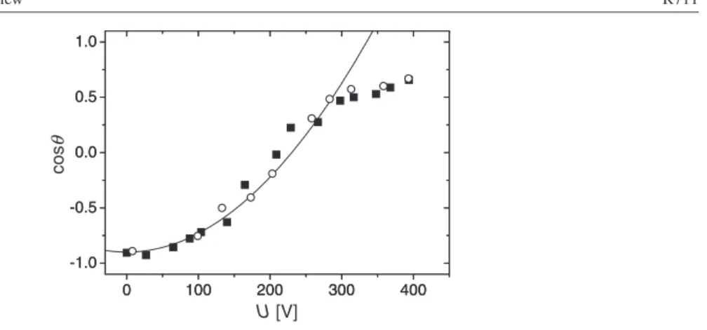
Figure 3. Contact angle versus applied (RMS) voltage for a glycerol–salt (NaCl) water droplet (conductivity: 3 mS cm−1; AC frequency: 10 kHz) with silicone oil as the ambient medium.
Insulator: Teflon AF 1601 (d ≈ 5µm). Note thatθY is almost 180◦ for this system. Filled
(open) symbols: increasing (decreasing) voltage. Solid line: parabolic fit according to equation (8) (reproduced from [52]).
solid–insulator interface (capacitancecH) and the dielectric layer withcd=ε0εd/d (εdis the dielectric constant of the insulator). SincecdcH, the total capacitance per unit areac≈cd. With this approximation, we neglect the finite penetration of the electric field into the liquid, i.e. we treat the latter as a perfect conductor. As a result, we find that the voltage drop occurs within the dielectric layer, and equation (5) is replaced by
σeff
sl (U)=σsl−ε0εd 2d U
2. (7)
(Here and in the following, we assume that the surface of the insulating layer does not give rise to spontaneous adsorption of charge in the absence of an applied voltage, i.e. we set Upzc=0.) In this equation the entire dielectric layer is considered part of one effective solid– liquid interface [30] with a thickness of the order ofd, i.e. in practice typically O(1µm). In that sense, the interfacial energy in equation (7) is clearly an ‘effective’ quantity. Combining equation (7) with equation (3), we obtain the basic equation for EWOD:
cosθ =cosθY+ ε0εd 2dσlv
U2=cosθY+η. (8)
Here, we have introduced the dimensionless electrowetting numberη=ε0εrU2/(2dσlv), which measures the strength of the electrostatic energy compared to surface tension. The ratio in the middle part of equation (8) is typically four to six orders of magnitude smaller than that in equation (6), depending on the properties of the insulating layer. Consequently, the voltage required to achieve a substantial contact angle decrease in EWOD is much higher.
Figure 3 shows a typical experimental example. As in many other experiments, equation (8) is found to hold as long as the voltage is not too high. Beyond a certain system dependent threshold voltage, however, the contact angle has always been found to become independent of the applied voltage [31–37]. This so-called contact angle saturation phenomenon will be discussed in detail in section4.
2.2.2. Energy minimization method. For EWOD, equation (8) was first derived by Berge [24]. His derivation, however, was based on energy minimization rather than interfacial thermodynamics: the free energy F of a droplet in an EWOD configuration (figure 1) is
composed of two contributions—in addition to the interfacial energy contribution Fif that appeared already in equation (1), there is an electrostatic contributionFel:
Fel=12
E(r)· D(r)dV. (9)
E(r)andD(r)=ε0ε(r)E(r)denote the electric field and the electric displacement atr·ε(r) is the dielectric constant of the medium at the locationr. The volume integral extends over the entire system. As in the previous section, the liquid is considered a perfect conductor; hence surface charges screen the electric fields completely from the interior of the liquid and the integral vanishes inside the droplet.
Before performing the minimization of the free energy, we have to identify the correct thermodynamic potential for electrowetting. In electrical problems, there are two limiting constraints: constant charge and constant voltage. The corresponding thermodynamic potentials are related by a Legendre transformation [38]. In electrowetting, the voltage is controlled. The thermodynamic potential corresponding to this situation is given by
F=Fif −Fel= i Aiσi−pV −12 E(r)· D(r)dV. (10) Before computing the contact angle decrease, one usually introduces another simplification: the electrostatic energy may be split into two parts. The first part arises from the parallel plate capacitor formed by the droplet and the electrode, withC = cdAsl. The second part is due to the stray capacitance along the edge of the droplet. The fringe fields are mainly localized within a small range around the contact line. Therefore, their contribution to the total energy is negligible for sufficiently large droplets. (In section2.3.1, we will consider the effect of fringe fields in more detail.) Hence, we findFel≈CU2/2=ε0εdU2Asl/(2d).
Apart from this formal explanation, the negative sign in equation (10) can also be understood intuitively by considering the entire system consisting of both the droplet and the power supply (the ‘battery’) required to apply the voltage. Upon connecting the initially uncharged droplet to the battery, the chargeδQflows from the battery(δQb = −δQ)to the droplet (and to the electrode). The work done on the droplet–electrode capacitor is given by δW = U(Q)δQ = Q/CδQ, with U(Q)being the charge dependent voltage on the capacitor. The electrostatic energy stored in the droplet in the final state isEdrop =
δW = Q2/(2C)=CU2
b/2. The work done on the battery isδWb=UbδQb= −UbδQ. In contrast toU(Q), the battery voltageUb is constant, such that we obtain a release of electrostatic energy ofEbatt = δWb = UbδQb = −
UbδQ = −CUb2. Hence the net electrostatic contribution to the free energy is−CU2
b/2. Electrowetting is thus driven by the energy gain upon redistributing charge from the battery to the droplet. The contact angle decreases because this increasesCand thus allows for the redistribution of even more charge.
For homogeneous electrodes, the free energy thus reads F=Alvσlv+Asvσsv+ Asl σsl−ε 0εdU2 2d −pV. (11)
Equation (11) has the same structure as the free energy in the absence of electric fields (equation (1)). On comparing the coefficients, the electrowetting equation (8) is rediscovered. As in the previous section, this derivation is based on the assumptions that (i) theσiare voltage independent, (ii) the liquid is perfectly conductive, and (iii) contributions from the region around the contact line (due to fringe fields) can be neglected. An important additional insight from this derivation is the fact that the energy gain in electrowetting is actually taking place in the battery, i.e. quite remotely from the droplet itself. This illustrates again the effective character of the definition in (equation (7)).
2.2.3. Electromechanical approach. Both methods discussed so far predict the same contact angle reduction. However, they do not provide a physical picture of how the contact angle reduction is achieved in mechanical terms. Such a picture can be obtained by considering the forces exerted on the liquid by the electric field. These forces contain contributions due to the response of the free electric charge densityρfand the polarization density in the presence of electric field gradients. This approach was introduced to the field of electrowetting by Joneset al[34,39] and recently reviewed by Zeng and Korsmeyer [4]. In the case of simple liquids, one of the most frequently used formulations is the Korteweg–Helmholtz body force density [38] fk =ρfE− ε0 2 E 2∇ε+∇ ε 0 2 E 2∂ε ∂ρρ (12) whereρandεare the mass density and the dielectric constant of the liquid, respectively. The last term in equation (12) describes electrostriction and can be neglected in the present context. The net force acting on a volume element dV of the fluid is obtained by a volume integration over equation (12). As a fundamental consequence of momentum conservation, the same force can also be obtained by an integration along the surface of dV over the momentum flux density of the electric fields, i.e. the Maxwell stress tensor. It seems particularly appropriate because in the perfect conductor limit of electrowetting the entire ‘body’ force actually acts at the surface: ρf is zero within the bulk, and free surface charges screen the electric field from the interior. The second term on the rhs of equation (12), the so-called ponderomotive force density,∝∇ε, vanishes everywhere except at the surface. Neglecting electrostriction, the Maxwell stress tensor consistent with equation (12) is [38]
Tik =ε0ε(EiEk−12δikE2). (13)
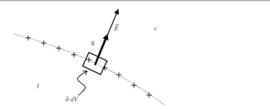
Here,δik is the Kronecker delta function, andi,k =x,y,z. Let us now consider a volume element dV at the liquid–air interface of a perfectly conductive liquid droplet (see figure4). The tangential component of the electric field at the surface vanishes and the normal component is related to the local surface charge density byρs =ε0E· n, wherenis the (outward) unit normal vector. Furthermore,Evanishes within the liquid. To obtain the net force acting on the liquid volume element, we calculate
Fi =
TiknkdA (14)
using the Einstein summation convention. We find that the only non-vanishing contribution is a force per unit surface area dAdirected along the outward surface normaln:
F/dA=Peln= ε0 2 E 2n= ρs 2 E (15)
where we have introduced the electrostatic pressurePel=ε0E2/2 acting on the liquid surface. Pelis thus a negative contribution to the total pressure within the liquid.
How does this local pressure at the surface affect the contact angle of a sessile droplet? The solution of the problem requires a calculation of the field (and charge) distribution along the surface of the droplet. Far away from the contact line, the charge density at the solid–liquid interface isρsl=ε0εdU/dand the liquid–vapour surface charge density vanishes. As the three-phase contact line is approached, both charge densities increase due to sharp edge effects, as first pointed out in [31]. The force arising from the charges at the solid–liquid interface leads to a normal stress on the insulator surface, which is balanced by the elastic stress. The forces at the liquid–vapour interface, however, contain both a vertical and a horizontal component pulling on the liquid. Kang [40] assumed that the droplet remains wedge shaped and calculated the net horizontal force acting on the liquid by integrating the horizontal component of equation (15)
l
∂ dV n
v E
Figure 4. Force acting on a volume element dVat the liquid–vapour interface with surface charges (‘+’). Solid box: area for surface integral.
along the liquid–vapour interface9. The field and charge distribution are found by solving the Laplace equation for an electrostatic potentialφwith appropriate boundary conditions. For the wedge geometry, an analytic solution can be obtained using conformal mapping as first described by Valletet al[31] in the context of electrowetting. Both the field and charge distribution are found to diverge algebraically upon approaching the contact line. The resulting Maxwell stress is thus maximal at the contact line and decays to a practically negligible value at a distance of a fewdfrom the TCL [40]. Integrating the horizontal component of the Maxwell stress, we obtain the net force acting on the droplet. For the horizontal component, the result reads Fx = ε0εd 2d U 2=σ lvη. (16)
Given the rapid decay of the Maxwell stress, this force can be considered as localized at the contact line, in a coarse grained sense—on a length scale much larger thand. Expression (16) can thus be used in the force balance at the contact line in the spirit of Young. As a result, we rediscover equation (8) for the third time. All three methods are thus equivalent.
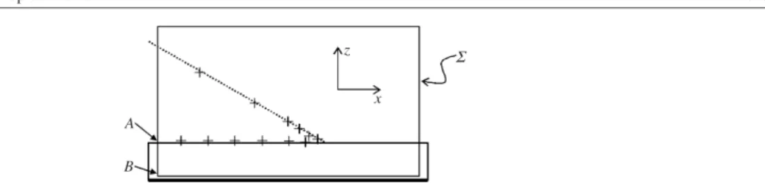
It is worth pointing out that the result in equation (16) can be obtained much more easily if we presuppose that the forceislocalized close to the contact line, as we did implicitly in the previous section when we neglected the contribution of fringe fields. Adapting the ideas of Joneset al[34,35,39,41], we can calculate the net force by choosing a sufficiently large box around the contact line (see figure5) that the electric field vanishes along most sections of the closed area. For such a box, only the section along A–B (in figure5) contributes to the integral in equation (14). As a result, we obtain exactly the same expression as equation (16). This means in particular that the net force pulling on the contact line is independent of the droplet shape. The result also implies that the edge of any non-deformable, perfectly conductive body would experience exactly the same force [4]. This is in fact not surprising since the net force calculated by integrating the Maxwell stress tensor must be the same as the one obtained by minimizing the energy: the gain in electrostatic energy upon moving the contact line in figure5by dxis given by the increment in the solid–liquid interfacial area. The contribution of the fringe fields remains constant—independent of the surface profile. (A derivation of the electrowetting equation that makes use of this argument was given in [32].) This shape independence of the force also implies that the contact angle reduction and the force should be regarded as independent phenomena [42].
9 We will see in section2.3.1[43] that this assumption is not correct. However, the main conclusion with respect to
A B
z x
Σ
Figure 5. Integration box for the calculation of the net force acting on the contact line.
2.3. Extensions of the classical electrowetting theory
2.3.1. Fine structure of the triple line. In the previous section, we discussed the response of the liquid on a mesoscopic scale. The impact of the fringe fields on the liquid surface in the vicinity of the TCL was ignored. If we look at the surface profile within that range, the liquid surface is expected to be deformed, as first noted by Valletet al [31]. In order to calculate the equilibrium surface profile, Buehrleet al[43] proceeded in analogy with conventional wetting theory in the presence of molecular forces ([26]; see also section2.1): in mechanical equilibrium, the pressurep across the liquid–vapour interface must be independent of the position on the surface. Therefore any electrostatic pressurePel(r)=ε0E(r)2/2 close to the TCL must be balanced by an additional curvature of the surface such that
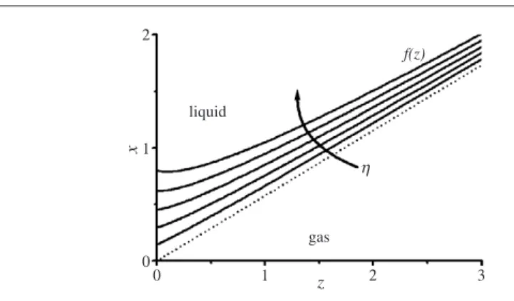
σlvκ(r)−Pel(r)=p=const. (17) Compared to conventional wetting theory, there is one major difference: while the disjoining pressure at a given positionrdepends only on the film thickness at that position [26], the electric field and thusPel(r)depends on the global shape of the droplet. Thus the droplet shape and the field distribution have to be determined self-consistently. Buehrleet al[43] addressed this question for the case of droplets of infinite radius. They chose an iterative numerical procedure, which involved a finite element calculation of the field distribution for a trial surface profile followed by a numerical integration of equation (17) to obtain a refined surface profile. The calculation was a two-dimensional one, i.e. possible modulations of the profile along the contact line were not included. The procedure was found to converge to an equilibrium profile after a few iteration steps. The following main results were found. (i) The surface profiles are indeed curved, as sketched in figure6. The curvature of the surface profiles and thus the electric field diverges algebraically at the TCL, as in [40] (with a different exponent, however). (ii) The asymptotic slope of the profile at the substrate remains finite and corresponds toθY, independently of the applied voltage. This is only possible because the divergence of the curvature is very weak. In fact, Buehrleet al[43] confirmed analytically thatPel∝rνwith an exponent−1< ν <0. (iii) The apparent contact angleθis in agreement with the electrowetting equation (equation (8)) up to the highest values of η investigated (corresponding toθ = 5◦). In view of the discussion in the previous section, this result is not unexpected. It also implies that contact angle saturation does not occur within a two-dimensional electromechanical model—in contrast to some arguments in the literature [40]. Recently, Papathanasiou and Boudouvis repeated the same calculation for droplets of finite size using a slightly different numerical scheme [36]. Except for small deviations from the electrowetting equation, which may be due to the finite size of their system, they reproduced most of the results presented in [43].
Despite the striking difference between the apparent contact angle and the local one at the contact line, the calculations showed that the surface distortions are significant only within a rather small region of O(d)around the TCL. From an applied point of view, this allows for
2 1 0 0 1 z 2 3 x gas liquid f(z) η
Figure 6. Equilibrium surface profiles (θ=60◦;η=0.2,0.4, . . . ,1.0;εd=1). Reprinted with
permission from Buehrleet al[43]. Copyright 2003 by the American Physical Society. the comforting conclusion that the simple models, as described in section2.2, are sufficient as long as the phenomena of interest occur on a length scale larger thand.
2.3.2. Electrolyte properties. Typical liquids used in electrowetting are aqueous salt solutions. They are conventionally described as perfect conductors with surface charges perfectly screening any external electric field. Microscopically, however, external fields are screened by an inhomogeneous distribution of ions close to the electrolyte surface. For typical ion concentrations, the penetration depth of the electric field is of the order of a few nanometres, given by the Debye lengthκ−1, withκ = (nb
iqi2)/ε0εlkBT. (The sum runs over all the
ionic speciesi, withnb
i andqi being the bulk concentration and the charge of theith species. kBis the Boltzmann constant andT is the temperature.) The local ion concentration and the electrostatic potentialφare coupled via the Poisson–Boltzmann equation [28]
∇2φ= −
i qinbi ε0εl
exp(−qiφ/kBT). (18)
Within this framework, the osmotic pressure
=nbikBT(exp(−qiφ/kBT)−1) (19)
of the ions has to be taken into account as an extra contribution to the free energy, such that the last term in equation (10) is replaced by [44]
Fel= 1 2ED+ dV = ε0εl 2 (∇φ) 2+ dV. (20)
In order to calculateFel, a solution of the Poisson–Boltzmann equation is required. For two specific situations the relation betweenandφcan be simplified considerably: when qφ/kBT 1, the Poisson–Boltzmann equation (as well as the expression for) can be linearized. In this case, one obtains=ε0εlκ2φ2/2. One should note thatkBT/e≈25 mV (e: elementary charge) at room temperature. Hence the applicability of the linearized Poisson– Boltzmann equation is limited to situations where the potential dropwithin the liquidis rather small. (While this is usually fulfilled in the centre of the droplet, deviations should be expected close to the TCL, where the electric field strength diverges (see the preceding section).) The second simple situation corresponds to having monovalent salt solutions withq1= −q2=z e (z: valency) andnb1=nb2. In this case, hyperbolic sine and cosine terms appear in equation (18) and in the expression for, respectively.
If we consider only the contributions of these terms to the energy per unit area of the solid– liquid interface (i.e. neglecting fringe field contributions), the problem is a one-dimensional one. Using appropriate boundary conditions (fixed potentials on the electrode and in the bulk liquid), analytic expressions for bothφandFel/Aslcan be obtained. The latter is a correction to the electrostatic contribution in equation (11), which ultimately leads to a correction to the electrowetting numberηin the electrowetting equation (8). More specifically, one obtains for the linearized Poisson–Boltzmann equation [45]
ηlin=η· 1 1 +εdλ/εld
(21) whereλ=κ−1. In the case of monovalent salts, the result is
ηmv =η· (1−φ0)2+ 16κd ν2 εl εd sinh2(νφ0/4) (22) whereν = eU/kBT. φ0 is the potential (in units ofU) at the solid–liquid interface. It is given by the solution of the equation 1−φ0−(2εlκd)/(εrν)·sinh(νφ0/2) = 0 (constant potential boundary conditions [45]). Withλdin typical experiments, it is obvious that the correction in equation (21) is small. Numerical solutions forφ0show that the same is true for the correction in equation (22). As already indicated in section2.2.1, corrections due to the double layer thus have a rather weak effect on the apparent contact angle.
Kanget al[46,47] as well as Chou [48] went one step beyond the above calculation and analysed specifically the contribution arising from the vicinity of the TCL. They calculated the electrostatic contribution to the line tension τe, i.e. to the excess free energy per unit length on the contact line. This excess energy arises from the overlap of the double layers originating from the solid–liquid and from the liquid–vapour interfaces. In [46], analytical results forτewere obtained for wedge-shaped surface profiles within the linear approximation of the Poisson–Boltzmann equation.τewas found to be of the same order of magnitude as the molecular line tension, i.e. 10−12−10−10 J m−1. Numerical solutions for the full non-linear Poisson–Boltzmann equation produced similar results. Like the line tension of molecular origin, the impact of this electrostatic line tension will hence be negligible for droplets with a diameter of, for example, a hundred nanometres or more. This conclusion is supported by numerical calculations of equilibrium surface profiles based on the full Poisson–Boltzmann equation in analogy to the discussion in section2.3.1[45].
2.3.3. AC electric fields. The theoretical treatment of electrowetting as discussed so far was based on static considerations. In the case of slow variations of the applied voltage, the contact angle and droplet shape can follow adiabatically the momentary equilibrium values. If the AC frequency exceeds the hydrodynamic response time of the droplet (for typical millimetre-sized droplets at frequencies exceeding a few hundred hertz), the liquid response depends only on the time average of the applied voltage, i.e. the RMS value has to be used in equation (8). This statement is correct as long as the basic assumptions in the derivation of the Lippmann equation are not violated: one of them, the assumption that the liquid can be treated as a perfect conductor, however, breaks down upon increasing the frequency. While the dissolved ions can follow the applied field at moderate frequencies and thus screen the electric field from the interior of the liquid, they are not able to do so beyond a certain critical frequencyωc. Far belowωc, the liquid behaves as a perfect conductor; far above it behaves as a dielectric. (Electric field-induced actuation of liquids beyondωcis still possible. However, the forces in that range are dielectric body forces. For a review on dielectrophoresis; see [10].) For homogeneous bulk
l, ε1, σ1
d, εd, σd
Figure 7. Capillary bridge between bare and insulator-covered electrode (see the text for details).
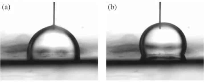
(a) (b)
Figure 8. Frequency dependence of contact angle (insulator: 1µm thermally grown Si oxide, hydrophobized with a monolayer of octadecyltetrachlorosiloxane). Droplet: salt (NaCl) water; conductivity: 0.2 mS cm−1; diameter: approximately 2 mm; ambient medium: silicone oil; URMS=50 V. (a) f =1 kHz. (b)f =20 kHz (reproduced from [83]).
liquids, the critical frequency for which ohmic and displacement currents are equal is given by [49]
ωc=
σl
εlε0
(23) whereσl andεl are the conductivity and the dielectric constant of the liquid, respectively. For an aqueous salt (NaCl) solution with a conductivity of 0.1 S m−1(≈10−4 mol l−1), we haveωc = O(108s−1). For demineralized water(σ = 4×10⁻⁶ S m−1) ωc is as low as 4×10³s−1. The relevant critical frequency in electrowetting, however, depends not only on the intrinsic properties of the liquid but also on the geometric and electric properties of the insulating layer. For instance, the characteristic time constantτcfor charge relaxation in the configuration sketched in figure7is given by10
τc=ε0
εd+εldl σd+σldl
. (24)
Using, for instance,d =1µm,l=1 mm,εd =2,εl=81,σd =0, andσl =0.1 S m−1 (as above), we obtain 2π/τ−1
c ≈ 4×10⁷ s−1, whereas for demineralized water, we have 2π/τ−1
c ≈1.6×10³s−1.
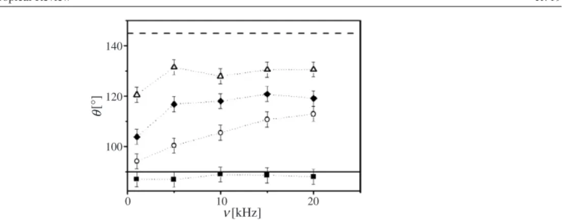
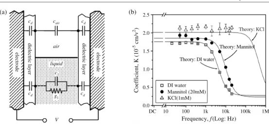
Figure8illustrates this breakdown of electrowetting at high frequency for a millimetre-sized droplet of demineralized water. At high frequency, a substantial fraction of the voltage that is applied to the wire drops within the droplet. Therefore, both the voltage at the contact line and thus the energy gain upon moving the latter are reduced. The continuous nature of the transition from conductive to dielectric behaviour as a function of frequency is illustrated in figure9for various salt concentrations.
The details of the contact angle response to the electric field are rather complex and geometry dependent when the field penetrates substantially into the liquid. The transition
10This equation can be derived using the boundary conditions for the electric and displacement fields at the solid–
liquid interface in combination with the continuity equation [49]. An alternative derivation based on equivalent circuit diagrams was described by Joneset al(e.g. [34]) for the specific caseδd=0.
140 120 100 0 10 20 [kHz] [ ° ] θ ν
Figure 9. Contact angleθversus frequency (see figure8for experimental details). Conductivity: 1850µS cm−1 (squares), 197 µS cm−1 (circles), 91µS cm−1 (diamonds), and 42 µS cm−1 (triangles). θY andθ are shown as dashed and solid lines, respectively. Reprinted from [50].
from low frequency electrowetting behaviour to high frequency dielectrophoretic behaviour is much better illustrated in experiments that measure the forces exerted by the electric fields. Jones et al performed a series of experiments in which they studied the rise of liquid in capillaries formed by two parallel electrodes at a distanceD, each covered with an insulator (figure10(a)) [35,41]. (Other examples where finite conductivity effects play a role will be discussed in sections5.3to5.5.) The authors modelled the liquid as a capacitor in parallel with an ohmic resistor; see figure10(a). The electric fields within the different materials can be calculated from elementary electrostatics. Using either the Maxwell stress tensor or the derivative of the total electrostatic energy with respect to the height of the liquid, a frequency dependent expression for the electric force pulling the liquid upwards is obtained. Balancing this force with gravity, Joneset al[35] obtained an expressionh =K(ω)U2with an analytical functionK(ω). The low and high frequency limits are given by
h = εdε0 4ρlgd D U2; ωωc (εl−1)ε0 2ρlg D2 U2; ωωc (25)
whereρl is the density of the liquid and g is the gravitational acceleration. The critical frequencyωc =2σ/(D·(2cl+cd))involves the capacitances per unit areaclandcd of the liquid and of the insulating layer, respectively. Figure10(b) shows K(ω) determined from a series of experimental height of rise versus voltage curves. Good agreement was achieved with model calculations based on independently measured liquid properties.
In addition to this frequency dependent reduction of the rise height, Joneset al[35] also observed a deviation from the predicted parabolic voltage dependence at high voltage. This observation is in qualitative agreement with earlier experiments [30], in which electrowetting-induced capillary rise was investigated using DC voltage. According to those authors, the deviation from parabolic behaviour inh(U)coincided with the onset of contact angle saturation on a planar substrate made of the same material.
3. Materials properties
In classical electrowetting theory, the liquid is treated as a perfect conductor. For aqueous salt solutions this corresponds to the limit of either high salt concentration or low frequency, as
cd cair cd c1 g1 cd cd air liquid V electrode
dielectric layer dielectric layer
electrode 2.5 2.0 1.5 1.0 0.5 0.0 DC 10 100 1k 10k 100k 1M Coefficient, K (10 -5 cm/v 2 ) (b) (a) Frequency, f(Log: Hz) DI water Mannitol (20mM) KCl(1mM) Theory: DI water Theory: Mannitol Theory: KCl
Figure 10. Pellat experiment: electrowetting-induced capillary rise. (a) Schematic set-up and electric equivalent circuit. (b) Frequency dependence ofK(w)for DI water, mannitol, and KCl. Reprinted with permission from [35].
discussed in the preceding section. The requirements regarding the concentration and nature of charge carriers are not very stringent. At low frequency (f <1 kHz), even demineralized water displays substantial electrowetting [35,50] (see also figures8 and10). Frequently, experiments are performed with salt concentrations of the order of 0.01–1 mol l−1. Most authors report no significant influence due to the type or concentration of the salt (see for instance [24,32]). However, Quinnet al[51] found systematic pH dependent deviations from equation (8), which they attributed to specific adsorption of hydroxyl ions to the insulator surfaces. Electrowetting was also observed for mixtures of salt solutions with other species (e.g. glycerol [52–54], ethanol [31,55]) without deterioration of electrowetting performance. In particular, electrowetting also occurs in the presence of biomolecules such as DNA or proteins [5,21,56,57] and has even been demonstrated for physiological fluids [5]. One complication with biological fluids is, however, that the performance can be affected by unspecific adsorption of biomolecules to the surfaces [56]. Adsorbed biomolecules generally reduceθYand increase contact angle hysteresis. Room temperature ionic liquids [55] were also shown to display electrowetting. Electrowetting is thus a rather robust phenomenon that depends only weakly on the liquid properties.
In contrast, the properties of the insulating layers are much more critical. Substantial activities have been aimed at optimizing the properties of these layers in order to minimize the voltage required for contact angle reduction. At the same time, the materials used should be chemically inert and stable in order to ensure reproducibility and a long lifetime. Two main criteria can be derived immediately from equation (8): first, the contact angle at zero voltage should be as large as possible, in order to achieve a large tuning range and, second, the dielectric layer should be as thin as possible. The first choice can be met by either using an intrinsically hydrophobic insulator, such as many polymer materials, or by covering hydrophilic insulators with a thin hydrophobic top coating. One possible top coating is self-assembled monolayers (e.g. silanes on glass or SiOx) [54]. More frequently, however, thin layers of amorphous
fluoropolymer (Teflon AF or Cytop) are used. These materials can be deposited by spin coating or by dip coating. Depending on the solution concentration and on the deposition parameters, layers with a thickness ranging from a few tens of nanometres to several micrometres [58] can be produced. Apart from being hydrophobic, Teflon-like layers can be prepared as very smooth
200 150 100 50 0 0 2 4 6 8 10 required EW voltage UBD d [µm] U [V]
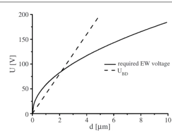
Figure 11. Electrowetting and dielectric breakdown voltage versus insulator thickness. Solid line: voltage required for a contact angle decrease from 120◦ (0 V) to 70◦ (forεd =2;σlv=
0.072 J m−2). Dashed line: critical voltage for dielectric breakdown (for EBD=40 Vµm−1).
with very small contact angle hysteresis (<10◦for water in air). The material is chemically inert and resists both acids and bases. Seyrat and Hayes [58] developed a preparation protocol that leads to very homogeneous Teflon AF layers with high dielectric strength(≈200 Vµm−1). Furthermore, amorphous fluoropolymer has become very popular, not only as a top coating but also as an insulating layer [19,20,51,53,58–60].
The critical materials parameter for the insulator is its dielectric strength, or the breakdown field strength EBD. This number limits the minimum thickness of the insulating layer: the voltage required to achieve a desired variation of the contact anglecosθis given by [58]
U(cosθ)=(dσlvcosθ/ε0εr)1/2. (26)
Dielectric breakdown occurs atUBD = Ecd. The competition between the two effects is illustrated in figure11. The intersection between the square root function and the straight line determines the minimum insulator thickness required to obtain a certaincosθ for a given dielectric strength—implying a corresponding minimum voltage. The latter can only be reduced by improving the dielectric strength or by using a different material. There are two limitations to this procedure: (i) in view of the diverging electric fields close to the contact line, the breakdown voltage may be exceeded locally, althoughU/d is still smaller thanEBD; and (ii) the dielectric strength of thin layers may differ from the corresponding bulk values [58].
Popular inorganic insulator materials include SiO2[34,56,61–64] and SiN [61,65,66]. Thin layers with a high dielectric strength can be produced using standard vacuum deposition or growth techniques. In combination with a hydrophobic top coating, they perform well as electrowetting substrates. Compared to Teflon AF (as an insulator), they also offer the advantage of a higher dielectric constant, which contributes to reducing the operating voltage further (see equation (26)). The dependence on the dielectric constant prompted Moonet al [61] to study thin layers of a ferroelectric insulator (barium strontium titanate (BST)) with a specifically high dielectric constant ofεd =180. For a 70 nm BST layer covered by 20 nm Teflon AF, they achieved a contact angle reduction of 40◦with an applied voltage of 15 V.
Polymer materials that were used in previous electrowetting studies include parylene-N and parylene-C [22, 30, 32, 35, 37, 41, 67], conventional Teflon films [31, 67, 68], polydimethylsiloxane (PDMS) [69,70], as well as various other commercial polymer foils of variable surface quality [31,69,71,72]. Parylene films are deposited from a vapour phase of monomers, which polymerize upon adsorption onto the substrate. The surfaces are known to be chemically inert and robust and display a high dielectric strength (200 Vµm−1; [30]).
In electrowetting, Parylene is almost exclusively used in combination with hydrophobic top coatings. One important advantage of the Parylene coatings is that the vapour deposition process allows for uniform conformal coatings on topographically patterned substrates, including the interior of capillaries [22].
Recently, Chiou et al [73] presented an interesting new approach making use of a photoconductive material, which allowed them to switch the electrowetting behaviour optically—a process the authors termed ‘optoelectrowetting’. The advantage of this approach is that individual addressing of electrodes in a digital microfluidic chip does not require individual electrical connections to all electrodes (20 000 in [73]). Electrode activation is achieved by directing a laser beam onto the desired electrode.
4. Contact angle saturation
The parabolic relation between the observed contact angle and the applied voltage (equation (8)) was shown experimentally to hold at low voltage. At high voltage, however, the contact angle has always been found to saturate. In particular, no voltage-induced transition from partial to complete wetting has ever been observed. (On the basis of equation (8), such a transition would be expected to occur atUspread =(2σlvd(1−cosθY)/(ε0εd)). Instead,θ adopts a saturation valueθsat varying between 30◦ and 80◦, depending on the system [24,30–33,37,61,71]; see also figure3.) It has now become clear that the linear electrowetting models described in section2cannot explain the phenomenon of contact angle saturation [36,43]. However, the latter studies showed that the electric field strength diverges close to the TCL. Although the divergence is cut off at small length scales (κ−1, i.e. a few nanometres), the field strength is expected to reach very high values—several tens or hundreds of volts per micrometre. So far, no consistent picture of contact angle saturation has emerged. Nevertheless, a number of mechanisms have been proposed to explain various observations:
(i) Verheijen and Prins [32] found indications that the insulator surfaces were charged after driving a droplet to contact angle saturation. They suggested that charge carriers are injected into the insulators, as sketched in (figure12). These immobilized charge carriers then partially screen the applied electric field. In order to quantify the effect, they assumed that the immobile charges are located at a fixed depth within the insulating layer and that their density
σTis homogeneous within a certain range(≈d)on both sides of the contact line11. With these assumptions, they derived a modified version of equation (8):
cosθ =cosθY+ ε0εd 2dσlv
(U−UT)2, (27)
whereUTis the potential of the trapped charge layer outside the droplet, i.e.σT =ε0εdUT/d.
σTand, thus, alsoUT are unknown functions of the applied voltage that depend on the (non-linear) response of the insulator material. The authors determined these functions by fitting equation (27) to their experimental data. The result was self-consistent, but it was not possible to establish a correlation between this threshold behaviour and other known material parameters or a microscopic process that could be responsible for the charge trapping. Papathanasiou and Boudouvis [36] tried to establish such a correlation by comparing numerically computed values for the electric field strength at the contact line (averaged over a certain area) with the dielectric strength of a variety of dielectric materials used in electrowetting experiments. The authors reported good agreement with published experimental saturation contact angles. However, it
11These assumptions seem somewhat artificial for homogeneous dielectric layers. However, it should be recalled
(see section3) that many electrowetting experiments—including that of Verheijen and Prins [32]—are performed on composite substrates made of a thicker main insulating layer and a thin hydrophobic top coating.
vapour dA cos θ liquid V V insulator dA d dσL dσM σM σL θ vapour trapped charge dA cos θ liquid insulator dA d d1 d2 dσL dσM σM σT σT σL θ (a) (b) V σ M L
Figure 12. (a) Schematic picture of the virtual displacement of the contact line in the presence of a potential across the insulator. An infinitesimal increase in base area dAat fixed voltageV
changes the free energy of the droplet, as a result of a change in interface area and the placement of additional charge dσLand image charge dσM. (b) The virtual displacement of the contact line in
the presence of a sheet of trapped charge. Now, the infinitesimal increase dAalters the free energy not only via the charge distribution between the electrode and the liquid but also via the charge distribution below the vapour phase. Reprinted with permission from [32].
should be noted that the agreement is sensitive to the size of the box used to average the electric field. The specific choice of 100 nm in [36] is not obviously related to any physical length scale of the system (such asκ−1).
(ii) Valletet al[31] observed two other phenomena that can coincide with contact angle saturation. They found that the contact line of salt solution droplets luminesces at high voltage. Light was found to be emitted in a series of short pulses with durations of less than 100 ns. The wavelength of the emitted light was verified to correspond to known emission characteristics of several ambient gas atmospheres. Simultaneously with the optical observation, the authors measured the current in the system: a series of spikes occurred at the same time as the optical emission pulses, indicating discrete discharge events. Within reasonable error bars, the onset voltage for both processes agreed with the contact angle saturation voltage. Both effects were attributed to the diverging electric field strength close to the contact line.
(iii) In the same publication, Vallet et al [31] also reported another phenomenon that occurred only for low conductivity liquids (deionized water and water–ethanol mixtures). For
Figure 13. Contact line instability and emitted satellite droplets at high voltage. (Deionized water on silanized glass; droplet diameter:≈3 mm.) Note the liquid necks between the satellites and the large droplet (inset).
these liquids, the contact line was found to become unstable at high voltage leading to the ejection of small satellite droplets from the edge of the main droplet with a characteristic lateral spacing. This observation was later reproduced by Mugele and Herminghaus [54] for mixtures of water and glycerol (see figure 13). Qualitatively, this instability is due to the mutual repulsion of like charges at the contact line. Beyond a certain threshold voltage, surface tension can no longer balance the electrostatic repulsion and the emission of satellites sets in. Valletet alperformed a linear stability analysis of the contact line. For a sinusoidal perturbation of wavevectorq(deduced from the experimental spacing of the satellite droplets) they balanced the electrostatic energy per unit length of the contact line with the additional cost in surface energy. With some simplifying approximations, they found a stability limit that reproduced the experimentally observed onset of the instability. While the model seems to capture the essential physics, it leaves other aspects unresolved, such as the fact that the instability disappears upon the addition of salt [31] (or at least, the threshold voltage increases substantially [74]).
Finally, there are two other proposed mechanisms that do not refer to the field strength at the contact line: (iv) Peykovet al [37] suggested that equation (8) should fail whenσeff sl (see equation (7)) approaches zero. The idea is that the energy of the interface between two phases must always be positive for an interface to remain stable. However, this model has not received broad acceptance because it is not clear whether this criterion is applicable for the effectivesolid–liquid interfacial energy in electrowetting12.
(v) Contact angle saturation can also occur when either the assumption of a perfectly conductive liquid or a perfectly insulating dielectric or both are violated. In section2.3.3we saw already that finite conductivity effects reduce the impact of an applied AC voltage on the contact angle: when the voltage partially drops within the bulk of the droplet, the net force acting on the TCL is reduced. The same effect can occur for DC voltage if the dielectric layer is not perfectly insulating. Shapiro et al [33] analysed the field distribution within
12Recall that the electrostatic energy gain, which is responsible for the negative term in equation (11), takes place in
and around a spherical cap-shaped droplet assuming a finite resistivity ratio A=ρdd/(ρlR) (ρd, ρl: resistivity of the dielectric and the liquid; R: droplet radius). Their calculations showed that the potential drop within the droplet increases with decreasing contact angle, which causes saturation. Overall, the results seem to compare favourably to some published experimental data. However, the general relevance of the approach—in particular for large resistivity ratios—has yet to be demonstrated.
The diversity of explanations indicates that contact angle saturation is still not well understood. Most probably, there may be no unique explanation. It seems clear that diverging electric fields at the contact line can induce several distinct non-linear effects, each of which may independently cause saturation. Which effect dominates depends on the specific conditions of each experiment and identifying these conditions requires more work in the future.
5. Complex surfaces and droplet morphologies 5.1. Morphological transitions on structured surfaces
Classical electrowetting theory was developed for planar substrates with homogeneous electrodes. Applications in microfluidics, however, demand the use of structured substrates (see section7). In most cases, the substrates are planar and homogeneous but the electrodes are patterned. Sometimes, the surfaces are chemically patterned in addition and in some cases topographical structuring is also used [55,62,75]. In most applications one is interested in the behaviour of the liquid on a scale that is large compared to the insulator thickness. Hence, effects related to the field distribution close to the contact line can be ignored (as discussed in section2.3.1). The effect of electrowetting is then reduced to a variation of the surface wettability on top of the activated electrode(s). The handiness of equation (7) now becomes apparent: with this equation, electrowetting on patterned substrates is mapped onto conventional wetting of chemically (and/or topographically) patterned substrates. The free energyFof the system is simply given by [16]
F[A]=σlv Alv− cosθ(r)dAsl . (28)
Here, cosθ(r)=cosθY+η(r)withη(r)depending on the voltage applied to the electrode at the positionr. (As in section2, equation (28) has to be supplemented with a constraint of constant volume.) The equilibrium morphology of droplets in electrowetting can thus be calculated by the same methods as the morphology of droplets wetting structured surfaces in the absence of electric fields. The latter subject has attracted considerable attention in recent years both from an experimental and from a theoretical point of view. The presence of either chemical or topographical patterns on surfaces gives rise to complex liquid morphologies. Under favourable conditions, several morphologies may be (meta)stable simultaneously. Abrupt morphological transitions between such competing morphologies can be induced by varying the surface wettability (or some other external control parameter [13,16,18,19,76]). From an applied perspective, the richness of phenomena gives rise to new opportunities for controlling and manipulating the behaviour of liquids on surfaces. Fundamentally, these phenomena arise from the fact that the prescription of the surface pattern and the liquid volume alone leave substantial freedom for the system to adapt its shape. In particular, the contact angle can assume any value betweenθAandθB, when the contact line is pinned along the edge between two domains A and B with the respective contact angles [77].
Except for a few simple geometries, the morphologies of liquid droplets on patterned surfaces have to be computed numerically by minimizing the functional in equation (28)
Figure 14. Electrostatic repulsion between adjacent droplets. A voltage applied to the central stripe electrode (width 20µm) produces a protrusion at moderate voltage (91 V; left image). At high voltage (210 V; right image) the protrusions approach each other and flatten. Droplet coalescence is suppressed by electrostatic repulsion. Reproduced from [52].
(under the constraint of constant volume). A popular numerical tool is the public domain software package Surface Evolver [78]. Application of the Surface Evolver to electrowetting problems has been demonstrated by several groups [19,52,53,68].
There is one notable exception to the analogy between conventional wetting and electrowetting with patterned substrates: changes of the topology of the liquid are affected by long range electrostatic attraction or repulsion at the contact line. For instance, the coalescence of neighbouring droplets can be suppressed by electrostatic repulsion [25]. Figure 14 illustrates this effect for two adjacent droplets with a specific electrode geometry [52]. For opposing voltages, electrostatic attraction facilitates coalescence (and can even lead to spark generation [53]).
5.2. Patterned electrodes
The simplest patterned substrate on which droplets display a morphological transition is a hydrophobic surface (e.g.θ =180◦) with a stripe of variable wettability(θs). For moderate wettability contrasts, there is only one stable morphology, which is a droplet slightly stretched along the stripe. For stronger wettability contrasts (i.e. θs < θc, with θc being a volume dependent critical angle), a second morphology appears, namely a section of a cylinder with the contact line pinned along the edges of the stripe. Brinkmann and Lipowsky [18,76] determined a complete morphological diagram describing the stability of both morphologies as a function of the reduced liquid volume (in units of the cube of the stripe width) andθs (see figure15). Klingner and Mugele [19] verified this prediction experimentally using an electrowetting set-up with a stripe electrode. In order to reduce contact angle hysteresis and to achieve a high contact angle at zero voltage as in [18], they used a system of two immiscible liquids (droplets of salt water in silicone oil). The experiments confirmed the theoretical prediction rather well (see figure15).
Similar experiments using multilayer substrates with various patterned electrodes separated by dielectric layers were performed by Bienia et al [68]. For the geometrical conditions of those experiments no morphological transitions occurred. However, the authors proposed an approximate method for incorporating corrections due to field enhancement close to the edges of the electrodes into equation (28). Continuous morphological changes were also observed for droplets confined between two parallel electrodes at a distance D,