Exploration of Variable Importance and Variable selection techniques in presence of correlated variables

(1)

Rochester Institute of Technology

RIT Scholar Works

Theses

12-18-2019

Exploration of Variable Importance and Variable selection

techniques in presence of correlated variables

Sailee Rumao

[email protected]

Follow this and additional works at: https://scholarworks.rit.edu/theses

Recommended Citation

Rumao, Sailee, "Exploration of Variable Importance and Variable selection techniques in presence of correlated variables" (2019). Thesis. Rochester Institute of Technology. Accessed from

This Thesis is brought to you for free and open access by RIT Scholar Works. It has been accepted for inclusion in Theses by an authorized administrator of RIT Scholar Works. For more information, please contact

(2)

Rochester Institute of Technology

College Of Science

Department of Mathematical Sciences

Exploration of Variable Importance and

Variable selection techniques in presence of

correlated variables

Author:

Sailee Rumao

Supervisor:

Prof. Ernest Fokoue

A thesis submitted for the degree of

MS Applied Statistics

(3)

Abstract

Variable selection is of utmost importance in aviation safety where the data contains a large number of highly correlated predictors and flight safety has to be accurately predicted. Variable selection methods were not encouraged in medical research where the subject-matter knowledge is limited. For this reason, Genell, Anna Nemes, Szilard Steineck, Gunnar Dickman, Paul W. (2010) conducted simulated study to compare Bayesian Model Averaging and stepwise regression to motivate medical researchers to conduct automatic variable selection on their regression models and encourage them to take advantage of it. In this era of data science and Machine Learning, we have extended this comparative study by considering Machine learning algorithms. Various studies have shown that the Recursive feature elimination (RFE) algorithm reduces the effect of correlation on the variable importance measure and results in minimal prediction error. In this study, we compare RFE-RF, RFE-SVM and Bayesian Model Averaging (BMA) for simulated data in the presence of correlation by varying sample sizes (30,300) for 45 variables considering both cases n<p and n>p. Our results show that the percentage of selecting true predictors is highest for the RFE-RF model of all the three models. However, though the overall percentage of selecting true predictors is highest for RFE-RF, the estimated probability of selecting correlated true predictors is better for the Bayes in comparison to the other methods.comparison to the other methods.

(4)

Acknowledgements

I want to thank my advisor Dr. Ernest Fokoue for his constant motivation and support through-out my thesis research. I also want to thank Dr. Carol Marchetti and Dr. Robert Parody for being on my thesis committee and for their valuable time and feedback on my work. I want to extend special thanks to Shawna Hayes and all the staff members of the Statistics Department for prepar-ing me to complete this endeavor and makprepar-ing my journey at Rochester Institute of Technology a memorable one. Last but not the least, I want to thank my parents and my entire family for their love and support towards my aspiration to get the masters degree.

(5)

Signature Page

APPROVAL SHEET

Signed by the Thesis committee

Name Signature Date

Dr.Ernest Fokoue (Supervisor) Dr.Robert Parody (Committee member) Dr.Carol Marchetti (Committee member)

(6)

“Essentially, all models are wrong, but some are useful”

(7)

List of Figures

1.1 Various Variable selection methods that follow either of the three definitions are

reviewed in the paper(Wei, P., Lu, Z., Song, J. (2015)) . . . 10

1.2 Reprint from "Variable selection – A review and recommendations for the practicing statistician" by,Heinze,Georg Wallisch, ChristineDunkler, Daniela,(2018) . . . 13

2.1 Gregorutti, Baptiste ,Michel, Bertrand, Saint-Pierre, Philippe,(2017) . . . 16

3.1 Rodriguez-Galiano et al.,(2015) . . . 26

3.2 Basak Debasish,Pal Srimanta,Patranabis Dipak Chandra (2007) . . . 28

3.3 One-Dimension Linear SVR Source:Awad, Mariette Khanna, Rahul (2015) . . . 29

3.4 Susan Gardner,(2017) . . . 33

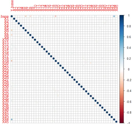
4.1 Correlation plot of the Baseline design, n= 300 . . . 36

4.2 Correlation plot of the Baseline design, n= 30 . . . 36

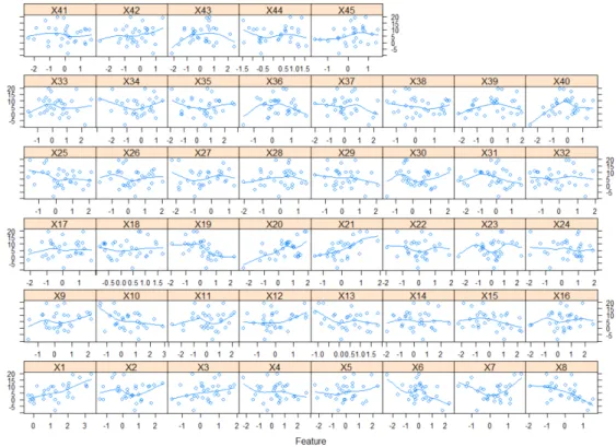
4.3 Scatter plot of the Independent variables with the dependent variables for the base dataset . . . 37

4.4 Scatter plot of the Independent variables with the dependent variables for the base dataset . . . 37

4.5 Correlation plot of the Block Covariance Matrix,n=300 . . . 40

4.6 Correlation plot of the Data Matrix generated from the block covariance matrix,n=300 40 4.7 Correlation plot of the Data Matrix generated from the block covariance matrix, n=30 41 4.8 Scatter plot of the Independent variables with the dependent variables for correlated data . . . 41

4.9 Scatter plot of the Independent variables with the dependent variables for correlated data . . . 42

4.10 R-square Adjusted . . . 43

5.1 Residual plot to examine gaussian distribution of errors of the simulated data . . . 47

(10)

5.3 Comparative Boxplots (n=30) . . . 49

A.1 Lasso Variable Importance . . . 52

A.2 Ridge Variable Importance . . . 53

A.3 Elastic net Variable Importance . . . 53

A.4 Random Forest Variable Importance . . . 54

A.5 BMA . . . 54

A.6 BMS Model Ranking . . . 55

(11)

List of Tables

4.1 Summary of Data Processes . . . 44

4.2 Method Comparison for Selecting True Predictors (n=300) . . . 45

4.3 Method Comparison for Selecting True Predictors (n=30) . . . 45

4.4 Probability of true predictors selected by correlation level (n=300) . . . 46

(12)

Chapter 1

Introduction

1.1

Motivation

This paper is motivated by the importance of variable selection in presence of highly correlated pre-dictors in the real-life problem of aviation safety that has been studied and published (Gregorutti, Baptiste, Michel, Bertrand, Saint-Pierre, Philippe,2017). It is a very sensitive issue to assure flight safety. This has to be done by evaluating all possible risks by studying the flight data parameters extremely minutely and faultlessly. The problem here is that the flight data recorders provide a large amount of raw data which contains a large amount of highly correlated variables. For this reason, it is of utmost importance to select the most important variables in order to get accurate predictions of any hazardous or unexpected events (Gregorutti, Baptiste, Michel, Bertrand, Saint-Pierre, Philippe,2017). Variable Importance Analysis and selection techniques were developed and studied independently in the fields of Statistics and Machine learning. The variable selection has a common problem of effect due to correlation which has also been studied independently. There has been extensive work done previously about the variable selection in the presence of highly corre-lated predictors. In this paper, I have explored and reviewed some of these works done previously and have re-addressed the issue of effect due to correlated predictors on variable importance. To the best of my knowledge, there has been no study to compare the effect of correlation on variable importance measured by the methods I have considered for the study. Our goal in this paper is to explore and compare the effect of correlation on different variable importance techniques to find if any of these methods give better results or is superior over other methods under any respective conditions. In part 1 of this paper, I have briefly discussed the theory of correlation and previ-ous work in variable importance analysis and variable selection. Further, I have talked about the theory of the methods chosen for this study and how variable selection is conducted using these methods. In the next part, I have conducted a simulation-based comparative study to understand

(13)

the effect of correlation on variable selection under different settings such as number of parameters (p), number of rows (n), correlation level and the level of signal-noise ratio (SNR) in the model output for each model that is built using the chosen Methods/techniques. This experiment is con-ducted using both Statistical and Modern Machine Learning techniques. The models are studied for their ability to select the true predictors in the presence and absence of correlation. The model performances are evaluated based on the root mean square error and visualized using boxplots.

1.2

Background

The modeling process is efficient and well-established if the variables are small, fixed and uncorre-lated or mildly correuncorre-lated. Variable importance analysis is conducted for feature selection to get precise reliable modeling results.

Let’s try to understand basics of variable importance by understanding the answers to following questions:

• What is Variable Importance?

• How is Variable Importance Defined?

• What are the different types of Variable importance measures or what are the different techniques used for variables selection?

• Why is variable selection important? In what fields does it play a significant role?

• What does variable importance affect?

Variable selection is done for multiple reasons and can be useful in different ways. Some of these are listed below in section 1.2.1. The goal of any data related project is to extract information or knowledge from the available data and to deduce significant inferences. Some practical applications of this might be to find a cure for a disease, to find loan defaulters, improvise web-search methods, for insurance modeling, to make strategic business decisions or any other real-life problem associated with data depending on the field of study and the purpose of the project. But the solution to a problem is never straightforward. Many applications have a large number of variables with only a few significant variables having relevant information required for the prediction or study of the project. There are numerous varying reasons for these non-contributing variables. However, in such cases, it is of utmost importance to consider only the important variables to complete the task efficiently and get a reliable outcome.

(14)

1.2.1

Reasons to use variable selection

• Variable selection has a significant advantage in a fast-paced world where this process enables the machine learning algorithm to train faster leading to decreased time required for training the model.

• Fewer variables contribute to less storage required in the system. Storage and fast processing time lead to significantly decreased costs involved in the process.

• It makes the model easily interpretable by making it less complex and giving the advantage of conducting meaningful data visualization to gain and showcase insights to the audience. • It plays a pivotal role in refining and boosting the performance of a model by choosing the

most significant variables contributing to the predictive accuracy of the model under study. • It helps to reduce over-fitting by eliminating redundant and irrelevant variables from the

model.

• Variable selection also increases model generalization.

• By keeping only the significant variables in the model, it makes the analysis more under-standable to gain knowledge about the process and help make important decisions quickly and confidently.

1.2.2

Definitions of Variable Importance

The variable selection process can be understood as the process of selecting a subset of most important variables which optimizes the objective function and minimizes the risk.

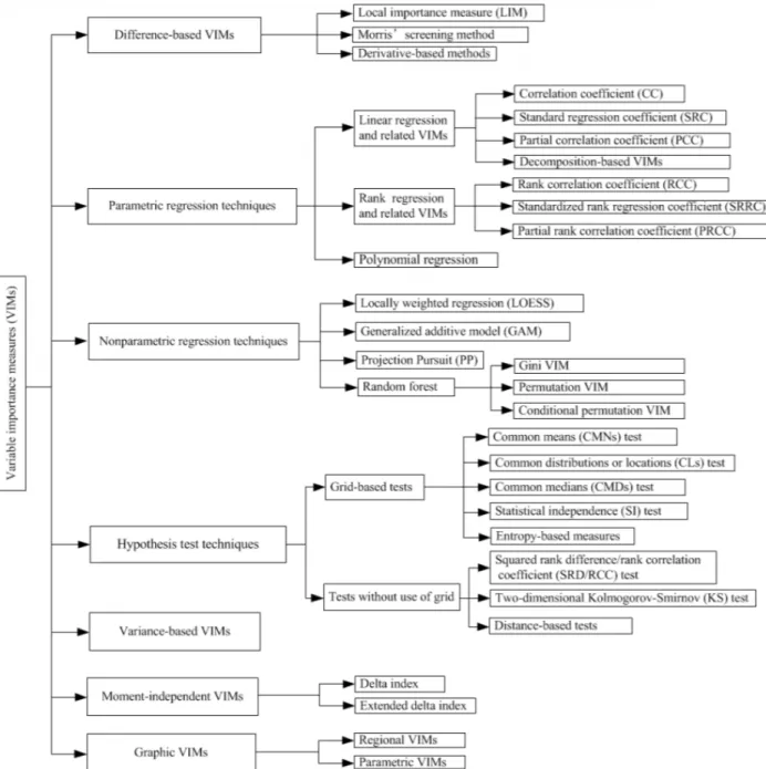
Variable Importance does not have a single consolidated definition. As these techniques were developed independently in multiple fields, it has been defined in different ways by these methods. In the review paper by Wei, P., Lu, Z., Song, J. (2015), they have classified all the Variable Importance measures into three categories and have defined it as follows:

• A calculated or estimated quantity that measures the change in the model performance with respect to the change in the predictor variables given to the model.

• A value that quantifies the variability contributed by one or more predictor variables to the variability of the model.

• A value that quantifies the intensity of association between the model outcome and the predictor variable individually or as a set.

(15)

Figure 1.1: Various Variable selection methods that follow either of the three definitions are re-viewed in the paper(Wei, P., Lu, Z., Song, J. (2015))

(16)

1.2.3

Types of Variable selection Methods

With the on-going research in the past, there have been numerous methods developed in this area to solve problems with different conditions. As discussed in the introduction, methods have been developed independently in statistics, machine learning and different fields of study. These methods can be broadly grouped and classified in the section below. Studying each of these methods in depth is out of the scope of this study. I have listed the approaches that researchers have utilized to tackle this problem so far.

Supervised Methods: 1. Filter Method

This method is based on calculating a particular statistical measure for a variable and scoring it to rank the variables. Considering a particular threshold for the measure computed, those variables that are greater than or less than the threshold are then selected or eliminated based on these scores. Here it is assumed that the feature that is greater than the threshold contains more infor-mation and is more relevant in comparison to others. The only drawback of this method is that the measure computed for a particular variable does not take into consideration its association with output variables for the ranking purpose and is independent of the output variables or the model output change. This method is usually statistically univariate and measures intrinsic properties of the variable, unlike the wrapper method which selects those variable as important which optimizes the objective function and improve the model performance.

Some examples of filter method are as follows:1. Information gain 2. Chi-square test 3. Fischer score 4. Correlation coefficient 5. variance threshold 6. PCA 2. Wrapper Method

This method behaves like a search problem. In this method, every single possible combination of all the available variables is tried to compute the predictive model performance. Each of the models is scored based on the model accuracy and compared to choose the best model with the best model performance built with the optimal subset of variables. The wrapper algorithm takes into account the association between the variable subset search and model selection based on the

(17)

model performance metric. It also has the potential to effectively deal with the correlated variables. (Sanz Hector,Valim Clarissa ,Vegas Esteban,Oller Josep M., Reverter Ferran (2018)).

The drawback of this method is that it has a higher risk of overfitting. Also, there might be a need to train and conduct cross-validation for each subset of variables to compare the model performance which is time-consuming and cost-expensive. Thus, the Filter method has an advantage over the wrapper method with regard to this aspect. This method can be methodological, stochastic or heuristic.

Some Examples of Wrapper Method are: 1. Forward selection method

2. Backward Elimination method 3. Stepwise Selection Method 4. Sequential Feature selection 5. Recursive Feature elimination

3. Embedded Method

This method works similarly to the wrapper method. However, embedded variable selection meth-ods incorporate model learning using the performance measure in the process of variable selection. This method includes calculation of the change in the objective function along with the search for the best variable for each iteration in the modeling execution. It selects the variables which minimize the fitting error along with the modeling procedure.

Some examples of embedded method are:1.LASSO (L1 Regularization) 2.Ridge

3.Elastic Net

4.Decision Trees (ID3, C4.5, and CART) 5.Random Forest

Unsupervised Methods:

1. Matrix Factorization 2. Clustering

(18)

1.2.4

Problems associated with Variable selection

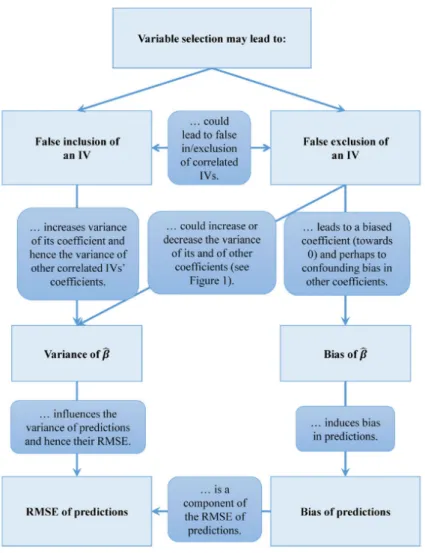
In addition to the benefits of variable importance analysis and variable selection discussed in section 1.2.1, there could be complications arising due to variable selection. These problems are statistically studied and are discussed in (Heinze, George Wallisch, ChristineDunkler, Daniela,2018). Refer to Figure 1.2. In this paper, they have also suggested possible solutions to these problems. They have mentioned some of these problems arising due to correlated predictors which are the center of our work.

Figure 1.2: Reprint from "Variable selection – A review and recommendations for the practicing statistician" by,Heinze,Georg Wallisch, ChristineDunkler, Daniela,(2018)

Some studies have also shown that sometimes the variable selection is not necessary and might not make a significant difference. Thus, before actually conducting variable selection, it is very im-portant to answer questions like"Should Variable selection be applied?" "Will it make a significant difference?" "Could there be any bad repercussions". Even after conducting variable importance analysis, it is crucial to conduct performance analysis, study Model sensitivity and test model sta-bility to see if things have improved or had they worsened, in order to avoid hazardous implications

(19)

of variable selection.

1.3

Thesis Scope

The scope of this study is limited to the linear regression framework for the two cases n<p and n>p where n is the number of observations and p is the number of variables. The number of observations for the case n<p is 30 and the number of observations for the case n>p is 300 and is fixed throughout the study. A crucial component of this research is to explore and analyze the behavior of the wrapper algorithms - Random forest and Support vector regression in the presence of correlation. Here the Pearson correlation coefficient is taken into consideration for the study and the correlation levels in the simulated data are set to three levels - uncorrelated variables, mildly correlated and highly correlated variables. Also, the experiments are conducted for a fixed low signal-noise ratio. Cross-validation to train the models under study is out of the scope of this study.

1.4

Organization

This thesis is organized in the following way. In Chapter 2, I have reviewed previous studies related to this area and introduced correlation and its types. In chapter 3, I have described the theory and mathematical concepts of all the models I have used in this study for comparison. In chapter 4, I have explained the simulation design procedure and have presented the results obtained from the experiments. In chapter 5, I have illustrated the choice of model performance metric and evaluated the results based on this metric. Finally, In chapter6, I have made conclusions from the study and made some remarks on the future scope for the experimentation.

1.5

Contributions

Although various studies have compared different variable importance measures and variable selec-tion methods, there is no research work to particularly compare the wrapper algorithms against the Bayesian method of variable selection for a linear regression framework. In this study, in addition to exploring various variable selection techniques, I have comprehensively analyzed these methods and provided an assessment of their ability to conduct variable selection. I have primarily studied the models for their ability to choose the true predictors effectively. I have evaluated the model performance of these methods using a common metric root mean square (RMSE) which would be an appropriate metric in this simulated study. The study has paved the scope for more research in this direction further for classification and for non-linear cases.

(20)

Chapter 2

Literature Review

2.1

Previous Work

Various importance analysis has been widely conducted considering different constraints and its behavior has been studied under different problems of which variable selection in high dimensional data had taken a lot of attention in this era. It includes popular research on the high-dimensional Microarray gene data where the challenge is to gain accurate disease-related information from the data that contains an enormous number of genes as variables and noise. The variable selection has also been studied in other disciplines to study specific problems of univariate constraints, re-dundancy, categorical/nominal variables, supervised /unsupervised classification and/or regression machine performances. Here in this paper, our focus is to study the effect of correlation on Variable importance analysis and compare variable selection methods RF-RFE, SVM-RFE and Bayesian Model averaging. But before we dive into it, let’s review some research papers to understand other work done in this area.

2.1.1

Synopsis of Variable importance and variable selection

Guyon, Isabelle De, Andre (2003) have discussed various methods of calculating variable impor-tance measures and criteria for variable ranking. These Methods include statistical techniques like mutual information, correlation co-efficient, variable subset selection methods (forward and back-ward selection), Clustering and Matrix Factorization. They have also briefly discussed validation methods like Statistical t-tests. They have mentioned the issue with regard to the choice of data proportions for training purposes and for validation purposes.Further, they have also brought up statistical issues like variance, multi-class problems. They have also mentioned that the results of sophisticated embedded or wrapper methods are not always significant especially in high di-mensional data sets. However, with decades of research work under these constraints, things have

(21)

improved and models like random forests have given significant results. They have concluded the paper by setting a layout for further work to create a unified benchmark for different settings in variable selection and by conducting performance evaluation by comparison with respect to a baseline model. In this paper, we have addressed the issue of the effect of correlation on variable selection by conducting an experiment on simulated data and comparing the variable selection with the baseline models.

Correlation and VIM in random forest

Gregorutti, Baptiste Michel, Bertrand Saint-Pierre, Philippe (2017) have studied variable im-portance using the random forest in the presence of correlation combined with recursive feature elimination and compared it with Non-recursive feature elimination (NRFE).In their study, they have shown that recursive feature elimination (RFE) with Random forest performs better than NRFE. The following figure Figure 2.1 represents the first ten variables selected by RFE and NRFE algorithms from the Landstad dataset over 100 runs.

(22)

The four colors in the figure represent four blocks of correlated variables. The horizontal line represents the block of variables selected and the vertical line represents the 100 iterations. From this study, they have concluded that the RFE algorithm is more consistent in selecting true predictors in comparison to the NRFE algorithm. These conclusions have motivated me to choose this model (Random forest - RFE) as one of the models for this comparative study for variable importance and variable selection.

Model selection in Medical Research: A simulation study comparing Bayesian Model Averaging and Stepwise Regression

Genell, Anna Nemes, Szilard Steineck, Gunnar Dickman, Paul W. (2010) have studied Bayesian Model averaging and stepwise regression for regression models both in the presence and absence of correlation. They have concluded that Bayesian Model averaging (BMA) performs better in selecting true predictors in comparison to the stepwise regression.

Numerous studies have been conducted to study variable importance using SVM-RFE for clas-sification. Ishak, A Ben, inspired from the SVM-RFE algorithm has introduced a new norm which is a tweak to the existing SVM-based metric for variable selection and found that this SVM norm performs well in variable selection even for models with small n and large p and has also shown that it is computationally faster. Sanz, Hector Valim, Clarissa Vegas, Esteban Oller, Josep M. Reverter, Ferran (2018) have studied SVM-RFE for non-linear kernals. Limiting to the scope of this study, I wanted to experiment and analyze the behavior of the SVM-RFE algorithm for the regression problem framework under consideration.

(23)

2.2

Correlation and Variable Importance Analysis

Correlation is the change between two variables that go along with each other. In other words, if with the change in one variable, the other variable also changes concurrently then the two variables are said to be correlated. This proclivity of variation between the two variables at the same time is called a correlation and indicates some kind of relationship between them. This relationship can go in the same direction or opposite direction. If so, the variables are termed as positively correlated or negatively correlated respectively. If there is no relationship between the two variables then the variables are said to have a neutral correlation.

Correlation between two variables is quantitatively estimated which informs us of the level of connection or association among the two variables. There are different methods to compute this numeric index. These methods are abstracted below:

2.2.1

Correlation and its types

• • • • • • • • • • • • • • • •

1. Pearson correlation coefficient (r):

This is the most widely used metric to gauge correlation in statistics. This index is practiced to measure the correlation strength also known as the effect size, between two continuous and linear variables. It can also be used for dichotomous categorical variables that are encoded in binary format. It is not a suitable index for categorical variables with more than two levels. For this index, the random error of the data should be equally spread over all the variables (Homoscadesticity).

The pearson correlation coefficient r is computed as follows:

rxz = n P xizi−P xiP zi p nP_x i2−(Pxi)2 p nP_z i2−(Pzi)2 (2.1) where,

rxz = Pearson correlation coefficient r between x and z

n= Total number of observations.

xi = ith observation of variable x.

zi = ith observation of variable z. −1≤rxz≤1

2. Kendall’s correlation coefficient (τ):

This index is used to measure the ordinal relationship between two variables. Thus it is the measure of the rank correlation of two variables. It is used as statistics for non-parametric tests to study if the two variables are dependent or independent.

(24)

τ= nc_n(n−nd −1) 2

(2.2)

where,

nc=number of concordant pairs nd=number of discordant pairs

3. Spearman’s Rank correlation coefficient (ρ):

This index is similar to the Kendall’s correlation coefficient and is suitable for the ordinal data. It is calculated as follows: ρ= 1− 6 P_d i2 n(n2₋₁₎ (2.3) Where,

ρ=Spearman’s rank correlation coefficient

di=The difference between the ranks for each observation between the two variables. n=Total number of observations.

Since the scope of our study is limited to the continuous and linear dataset, we have used Pearson’s correlation coefficient for this study.

Nicodemus, Kristin K. Malley, James D. (2009) have shown that the Random forest Gini in-dex is biased towards correlated variables and permutation-based variable importance measures are mildly impaired by correlation. Degenhardt, Frauke Seifert, Stephan Szymczak, Silke (2019) have inferred that recomputing variable importance recursively as in the RFE algorithm results in better results for correlated variables. They have also declared that the random forest vari-able importance measure Mean decrease in Gini Index is biased and that permutation varivari-able importance is not influenced by correlation. In addition to the above, Gregorutti, Baptiste Michel, Bertrand Saint-Pierre, Philippe (2017) have theoretically attested that permutation importance measure in the random forest is susceptible to correlation and should be recomputed after each variable is eliminated using the RFE algorithm. Therefore I have Incremental MSE (%IncMse) which is a permutation-based variable importance measure for the experimental study using the RFE algorithm.

(25)

Chapter 3

Methodology

3.1

Recursive Feature Elimination

Recursive feature elimination (RFE) and Non-Recursive feature elimination (NRFE) are types of Wrapper algorithms. Wrapper algorithms are succinctly described in section 1.2.3. These algorithms are computationally expensive but they do a full-scaled inspection with all possible combinations of the variables. This algorithm ranks variables according to the criteria and then traverses the best model based on it. The distinction in these techniques depends on two things:

• Computation of Variable importance measure.

• Computation of Predictive performance.

The differentiation between the two algorithms can be seen from the working of the two respec-tive algorithms paraphrased below:

Algorithm 1Non-Recursive Feature Elimination (NRFE)

1: Train the Model using all the variables

2: Rank the Variables using the variable importance measure

3: Calculate the Model Performance metric

4: Eliminate the least important variable

5: forall the remaining variablesdo

6: Train the Model again

8: Continue until convergence or no variables left

9: end for

10: Calculate Model performance metric for each Variable subsetVi

11: Choose the subset with best Model Performance as best subset of variables.

• Note in this algorithm that the rank is not re-calculated or updated each time a variable is eliminated and the model is re-built.This is the primary difference between NRFE and RFE.

(26)

Algorithm 2Recursive Feature Elimination (RFE)

1: Train the Model using all the variables

2: Calculate the Model Performance metric (MSE)

3: Calculate the Variable importance measure

6: Train the Model again

7: Calculate the Variable importance measure

10: end for

3.1.1

Recursive Feature elimination (RFE) vs Non-Recursive Feature

elimination (NRFE)

NRFE and RFE are compared in (Svetnik et al. ,(2004)) for real data sets where NRFE performs better. In (Gregorutti, Baptiste Michel, Bertrand Saint-Pierre, Philippe,2017) NRFE and RFE for Random forest are analyzed for simulated data in the presence of correlation. The results for this research show that RFE based on random forest performs more reliable than NRFE in the ubiquity of correlated predictors.

RFE algorithm updates the variable importance measure at each step of the backward elimina-tion approach iteratively.RFE warrants that the ranking of variables is consistent throughout each of the models by re-calculating it in each of the iterations. (Gregorutti, Baptiste Michel, Bertrand Saint-Pierre, Philippe,2017). In this study, I am eliminating one feature at a time. The stop-ping criteria are until there are two variables left which would be regarded as the most important variables.

The variable selection has a very prevalent issue of model instability. This issue can be best administered by the usage of bootstrap samples. In their paper, Gregorutti, Baptiste Michel, Bertrand Saint-Pierre, Philippe,2017, they demonstrate that RFE performs better than NRFE for simulated data. Therefore we have adopted the RFE over NRFE to conduct this experiment to examine different methods of variable selection.

(27)

3.2

Random Forest

Introduction

Random Forest is an ensemble learning algorithm. Ensemble learning models strive to reduce the model prediction errors as a result of the Bias Variance decomposition, by aggregating the performance of say, k models. There are two types of ensemble learning algorithms: Bagging and Boosting. Random Forest operates on the mechanism of the Bagging method.

Consider D =

n

Z1,Z2,· · · ,Zn

o

where Zi = (Xi, Yi) to be a learning data set where Xi = (Xi1,· · ·Xip)is the p-dimensional input vector andY = (Y1,Y2,· · ·Yn)is the response vector.

We know that the true prediction errorRis not known in reality. For this reason, we estimate this errorR using the sampleDas

R= 1 |D| P (Xi,Yi)∈D(Yi− ˆ f(Xi))2

And we would have M different estimators off,f1ˆ(·),· · ·fmˆ (·) wherem= 1,2,· · ·M computed from the k samples ofD

Here eachfmˆ (·)is called the Base learner.

Our goal is to find an estimator off with the smallest prediction error.

Assumef : function that models relationship betweenX andY ˆ f1(·),fˆ2(·),· · · ,fˆm(·) : M different estimators off Mathematically, ˆ f(agg)(·) = M X m=1 αmfmˆ (·) i= 1,2,· · ·M (3.1) Where,

(28)

Working:

Before we jump into the working of Random forest, Lets understand the Out of Bag Error (OOBE)

Out of Bag Error

Considerz∈_Dbe a random pair drawn fromDand

Consider bootstraped sample_D(m) _{of size n , then,} P r(z∈_D(m)₎_{= Proportion of observations from}

Dpresent in _D(m)=1−(1−1 n)

n _...(*) P r(z∈/_D(m)₎_{= Proportion of observations from}

Dnot present in_D(m)=(1−1 n)

n ₌_{P r}_[_On_]

...(**)

Asn→ ∞ , P r[On]→e−1 = 0.37

This implies that approximately one third of the training set is not used to build mth boot-straped base learner. This proportion is used to calculate the out of bag error.(used in random forest to estimate variable importance.)

Now letfˆ(m)₍_.₎_{be the base learner from}

D(m)_.

Then the out of bag error offˆ(m)_(·)_{is ,}

errO O B( ˆf(m)(·)) = Pn i=11(zi∈/D(m))`(yi,fˆ(m)(xi)) Pn i=11(zi∈/ D(m)) (3.2) where, 1(·) :Indicator function `(·,·) :Loss function

Thus, the OOB error for the ensemble is,

errO O B( ˆf(agg)(·)) = 1 M M X m=1 errO O B( ˆf(m)(·)) (3.3)

(29)

Random forest works on the foundation of bagging as described in the steps below:

The CART (decision tree for classification and regression) are known to be unstable for predictions subject to the training sample and may also tend to overfit the models. For these acumens, (Breiman,2001) developed the random forest as a significant improvement over the decision trees. The aggregation for the random forest is based on the predictions by all the trees built on all the bootstrap samples. The best split variable is determined based on the variable importance measure calculated for each variable in each bootstrap sample. The variable with optimal variable importance measure is chosen to be the split. This working can be well conceded from the steps below:

1. Bagging process

(a) Subset the datasetDn such that it has d variables from the original p-variables (Xj1, Xj2· · ·, Xj d): Subset of variables (where d < p).

Note that hereXj k are chosen without replacement

D(m) _{is an nxd matrix. Note that here m stands for the number of trees grown in the}

process.

(b) Pick bootstrap sample from _D(m)_{(This is done with replacement).}

(c) Construct base learner for_D(m)

2. Decide and compute for the Variable Importance Measure for_D(m)

(a) Set aside the bag of sample of size S =e−1n

(b) After fˆ(m)(·) is built which is the estimate for the mth tree of the total ntrees to be grown, calculate out of bag error i.e_EˆO O B (raw)

(c) For k=1 to d,

i. Perform permutation of column jk in OOB sample (shuffle the entries in column

jk)

ii. ComputeEˆ(k)O O B

iii. ComputeEˆO O B −Eˆ

(k)

O O B

3. To comprehend the outcome based on all the Base learners, the algorithm employs the majority vote for classification. For regression, the average value is utilized.

(30)

Random forest algorithm Variable importance measure

There are numerous variable importance measures like Gini-index, entropy, information gain, etc. For this research, I have used the package randomForest which computes these two variable importance measures IncMSE and IncNodePurity.Several studies have explicated that measures based on Gini-index are biased. (Degenhardt, Frauke Seifert, Stephan Szymczak, Silke (2019)) %IncMSE also known as the Mean decrease in Accuracy is said to be a very informative measure of importance. Thus, in this study, I have used IncMSE for this simulation study and correspondence.

• %IncM SE

This metric measures the increase in MSE of predictions when a variable j is permuted.It is also know as Mean decrease accuracy for classification problems.

The algorithm works computes IncMse in the following steps: 1. Grow regression forest.

2. Compute OOB-mse and call it mse0.

3. for 1 to j variables: permute values of variable j, Make predictions under this condition and compute OOB-mse(j)

IncMSE of j’th is (mse(j)-mse0)/mse0 * 100

Random Forest RFE algorithm

Many times in the case of correlated variables, models with a small subset of variables give good prediction performance. Since RFE recalculates the variable importance measure at each step, it takes into consideration the magnetism of correlated variables and picks the subset of variables most efficient in prediction. (Gregorutti Baptiste, Michel Bertrand, Saint-Pierre, Philippe (2017)) Now let us understand the implementation of the Random forest algorithm in the Recursive feature elimination mechanism from the steps in the algorithm outlined below.

(31)

Algorithm 3Random Forest -Recursive Feature Elimination (RF-RFE)

1: Train the Model using the Random forest algorithm described above for all the variables

3: Calculate the Variable importance measure %IncMse

4: Eliminate the least important variable based on the variable importance measure.

6: Train the Model again as in step 1.

7: Calculate the Variable importance measure IncMse

10: end for

11: Calculate Model performance metric (MSE) for each Variable subsetVi

In this algorithm, I am eliminating one variable which is least significant at a time. Then train the model repeatedly for the remaining variables and the variable importance measure is re-computed. I use the test data to make predictions every time and store the resulting root mean square error (RMSE) for each subset of the variable. For this experiment, I ran this algorithm 100 times and averaged the root mean squared error (RMSE) over these 100 iterations for each of the two data processes - Baseline and correlated.

(32)

3.3

Support Vector Regression (SVR)

Introduction

Support vector machines were introduced by Vapnik (1963). The two categories of SVM are Support vector classification(SVC) and Support vector regression (SVR). Since the extent of this study is confined to the regression framework with a continuous-valued response variable, we will only look at Support vector regression. A support vector machine is the generalization of the well-known portrait algorithm. This algorithm allows the machine to learn and generalize the data that it has not seen ahead. Statistics is the establishment of support vector machines and they operate on quadratic constraints to minimize the objective function which incorporates the cost function and the regularization function. The difference between regression and Support vector regression is that unlike regression support vector regression intends to minimize the generalization error which is a combination of training error and the regularization term. The regularization function is a term that controls the complexity of the hyperplane. (Basak Debasish, Pal Srimanta, Patranabis Dipak Chandra,(2007)) Support vector machines are known to apportion well with sparse data and are also apprehended to handle the overfitting of the models.

Working

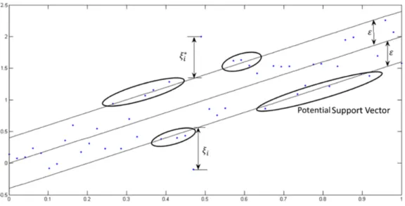
Support vector machines for classification are extended to support vector regression by adding an

−insensitive region encompassing the optimization function which is called the−tube. The goal is to find thetube such that it maximizes the number of data points in this tube and minimizes theinsensitive loss function.

(33)

Figure 3.2: Basak Debasish,Pal Srimanta,Patranabis Dipak Chandra (2007)

Just like the SVM for classification, in SVR we reach the hyperplanes by using a complex algorithm to depreciate the errors and maximize the margins.

The optimization function to be approximated is mathematically reproduced as follows,

y=f(x) =< w, x >+b=

M

X

j=1

wjxj+b y, b∈R,x,w∈RM (3.4)

The preceding equation is for one-dimensional data. If we have multi-dimensional data X then we can augment X with 1 and the mathematical equation of multivariate regression in equation 3.4 can be rendered as,

f(x) =    w b    >   x 1   =w >_x₊_b _x_,_w_∈_RM _(3.5)

The goal of support vector regression to minimize the loss function. The constraint here is to minimize the error between the predicted values of the function and the actual values. This commences to the minimization of the objective function beneath:

minw 1 2kwk

2

(34)

Figure 3.3: One-Dimension Linear SVR Source:Awad, Mariette Khanna, Rahul (2015)

In the Equation (3.6),

kwkMagnitude of the vector to the plane that is being approximated. ωis also called as the weight vector.

SVR uses theloss function to penalize the data points that are beyondfrom the coveted output. The value ofcircumscribes the width of the tube. Lower width ofindicates low error tolerance and a higher number of support vectors while a higher width ofindicated vice-versa. The choice of the loss function depends on the antecedent information concerning the data, signal to noise ratio and training complexity. In this instance, I have acknowledged the linear loss function also known as the L1 hinge loss which is defined as follows:

L(y, f(x, w)) =        0, |y−f(x, w)| ≤; |y−f(x, w)| −;, otherwise;. (3.7)

According to a few studies, asymmetrical loss function assists decrease the number of support vectors. As in the case of SVM, in order to take precaution against the outliers, slack variables (ξi+ξi∗)can be supplemented by the following the soft margin approach. Furthermore, a

regular-ization term C is added to the optimregular-ization function 3.6, Then the equation shifts to asymmetrical loss function that can be represented as follows:

minw 1 2kwk 2 +C n X i=1 (ξi+ξi∗) (3.8)

(35)

Under the following constraints,

yi−w>xi−b≤+ξi i= 1,2,· · ·n (3.9)

w>xi−b−yi≤+ξi∗ i= 1,2,· · ·n (3.10)

ξi, ξi∗≥0 i= 1,2,· · ·n (3.11)

Based on all the constraints, the optimization function is modified as follows:

L(w, ξi, ξ∗_i, λ, λ∗, α, α∗)=minw 1 2kwk 2 +C n X i=1 (ξi+ξi∗) + n X i=1 α∗i(yi−w>xi−b−−ξi)+ n X i=1 αi(−yi−w>xi−b−−ξi) + n X i=1 (λiξi+λ∗iξi∗) (3.12)

λi, λ∗_i, αi, α∗_i are non-zero real valued Langrange multipliers. (Awad, Mariette Khanna, Rahul,(2015)) Since the experimental data in this study is linearly separable, I am using linear kernal for this study such that,

f(x) =

n

X

i=1

(α∗_i −αi)k(xi,x) +b (3.13)

Where,k(xi,x) =φ(xi).φ(x)is the dot product denoting linear kernal.

SVM Variable importance measure

Variable selection in Support vector machines works on the principles of wrapper algorithm where it searches through all the subset of variables for training the dataset to find the best subset based on the accuracy of the model. In our study, we further extend this by computing the model per-formance on the test dataset using the RFE algorithm.

In Support vector machines the weight vectors represent the hyperplane. These vectors are orthog-onal to the hyperplane. The weight vectors are calculated using the dot product of the variable coefficients and the support vectors of the fitted model.

We have adopted these weight vectors to compute the variable importance measure for the support vector regression model in this research.

(36)

The SVM model is fit using the e1071 package in R Software. In this model, the epsilon is set to 0.9 and because our data is linearly separable, I have applied Linear Kernel.

SVM RFE algorithm

The SVM-RFE algorithm was proposed by Guyon et al. (2000) for selecting genes that are relevant for a cancer classification problem. The working of SVM-RFE is similar to that of RF-RFE and it contrasts in calculating the variable importance measure in addition to the model itself. It is illustrated in the subsequent steps below:

Algorithm 4Support Vector Machines- Recursive Feature Elimination (SVM - RFE)

1: Train the SVM Model using all the variables

3: Calculate the Variable importance measure support vector weights

4: Eliminate the least important variable with the minimum weight.

5: forall the remaining variablesdo 6: Train the Model again as in step 1.

7: Calculate the Variable importance measure support vector weights

10: end for

This algorithm also operates in an analogous way to that of RFE-Rf. The root means squared error (RMSE) is averaged over 100 iterations and plotted in the boxplots in the chapter for both the sample sizes (n=30,n=300) and both the data processes - baseline and correlated datasets. The minimum RMSE estimated in the process for each leave-one-out variable in the recursive feature elimination process additionally denotes the best variable subset size.

(37)

3.4

Bayesian Model Averaging

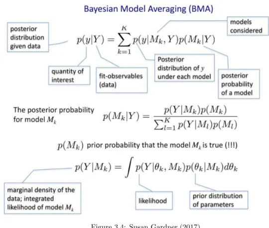
Bayesian Model Averaging follows undeviatingly from the Bayes Theorem. Bayesian Model Aver-aging (BMA) deals with Model skepticism. It scrutinizes all possible combinations of models in the model spaceM. From Bayesian Model, we know that we need to describe the prior probability to get the posterior probability. In this case, we need to define the prior distribution on the model spaceMto get the posterior distribution P(Mj|y)of each modelMj in the Model spaceM

From the posterior model probabilities, the best model is determined.It is the one with highest posterior probability. Choosing one best model based on this criteria and despising all other model can give fallacious predictions. Thus,Bayesian model averaging (BMA) deems for the posterior probability of the models as weights and builds a model by averaging posterior results from all the individual models in the model spaceM. (Steel, Mark F J (2011))

In other words, BMA resolves the predicament of Model uncertainty by estimating models for all possible combinations of the input variables X and by constructing a weighted average across all of them. For example,if X contains K input variables, then we would have2k_{variable combinations}

to be estimated.This accounts for a total of 2K _{models. The model weights for this process are}

obtained from the posterior model probabilities.

To make inference using BMA,a non- model specific quantity ∆is calculated by averaging all the models. This can be mathematically manifested as follows:

p∆|y= J

X

j=1

p∆|y,Mjp(Mj|y) (3.14)

In the above equation,pMj|y)is computed using bayes theorem and is as follows:

p(Mj|y) =py(Mj)p(θ|Mj) (3.15)

py(Mj): the Marginal likelihood ofMj together with the prior probability ofMj dentoted as

p(θj|Mj)

And thus, the marginal likelihood is defined as follows:

py(Mj) =

Z

p(y|θj, Mj)p(θj, Mj)dθj (3.16)

Let2K =J. Since the total number of modelJ(j = 1,2· · · J)can be very large and conse-quently it can be computational exhaustive to average over all the models, BMA performs sim-ulations using Monte Carlo Markov Chains sampler to deal with the Model spaceM There are other sampler methods like coin-flip importance sampling algorithm, branch, and bound method,

(38)

Bayesian Adaptive sampling approach (Steel, Mark F J(2011)) which are not used for our study.

Bayesian Variable importance measure

• For this research, I have adopted posterior inclusion probability (PIP) which is obtained by averaging across all the possible individual models.PIP is a measure that BMA calculates to indicate how likely it is for a variable to be included in the true model. Posterior inclusion probability is the mean of the posterior probabilities. This value calculated by the Monte Carlo Markov chain sampler in BMA.This measure gives us a reliable understanding of how well the data accommodates a particular variable and how much the variable is contributing to the response variable.

The Bayesian Model averaging (BMA) is concisely summarized in the following image.

Figure 3.4: Susan Gardner,(2017)

This algorithm is independent of the recursive feature elimination concept (RFE). It is replicated over 100 iterations just like the other two methods and the appearance of the important variables in each instance is recorded. The important variables are selected from the ranked features by the posterior inclusion probability above a threshold of 0.5.

(39)

Algorithm 5Bayesian Model Averaging

1: Compute Marginal Likelihood of each model.

2: Set the Model before distribution for each model.

3: Train the Bayesian model for each model and compute the posterior probability.

4: Perform MCMC simulations to sample the models with non-negligible posterior probability.

5: Fit the BMA model and Compute the posterior probability averaged over all the models.

6: Calculate the Model Performance metric (MSE).

7: Calculate the Variable importance measure posterior inclusion probability (PIP) that is ob-tained by averaging over all these models.

8: Eliminate the least important variable based on the posterior inclusion probability (PIP) by setting a threshold.

R package bms

• Used the default number of models: 500 to store the results from the best models and the default mcmc sampler in the package to experiment.

(40)

Chapter 4

Experimental Design and Analysis of

Different Methods

In this chapter, I have explained the simulation process on the methods described in Chapter 3.I begin by explaining the Simulation design.Further I have explained the experimental data generating process for each method.

4.1

Simulation Design

In this experiment we simulate two data sets for the purpose of comparison as suggested in the conclusion of (Guyon, Isabelle De, André Elisseeff,(2003)):the Baseline design which has the or-thogonal variables and the Correlated design which comprises of correlated variables.

A. Baseline data set

We simulate n=300 n=30 , p=45 i.i.d random normal and orthogonal variables from a multivariate Gaussian distribution

X ∼ N(µ,Σ(0)).

Here,

(41)

Figure 4.1: Correlation plot of the Baseline design, n= 300

(42)

Figure 4.3: Scatter plot of the Independent variables with the dependent variables for the base dataset

Figure 4.4: Scatter plot of the Independent variables with the dependent variables for the base dataset

(43)

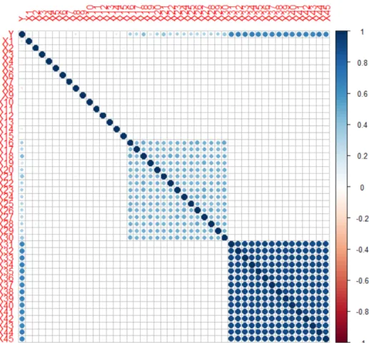
B. Baseline data set with correlation inducedSimilarly for this Data set, I have simulate n=300,p=45 i.i.d random normal variates from a multivariate Gaussian distribution

X ∼ N(µ,Σ).

Where,Σ =Block Covariance Matrix

such that the correlation levels are divided into three groups:

1. Orthogonal variables(X1(0), X2(0), X3(0),· · ·Xp1(0))∼N (µ,Σ(0))withρ= 0andp1= 15

Σ(0)=                 1 0 0 · · · 0 0 1 0 · · · 0 0 0 1 · · · 0 .. . . .. .. . . .. 0 0 0 · · · 1                 (4.1)

2. Mildly correlated variables(X1(0.5), X2(0.5), X3(0.5),· · ·Xp2(0.5))∼N (µ,Σ(0.5))withρ= 0.5 andp2= 15 Σ(0.5)=                 1 0.5 0.5 · · · 0.5 0.5 1 0.5 · · · 0.5 0.5 0.5 1 · · · 0.5 .. . . .. .. . . .. 0.5 0.5 0.5 · · · 1                 (4.2)

(44)

3. Strongly correlated variables(X1(0.9), X2(0.9), X3(0.9),· · ·Xp3(0.9))∼N (µ,Σ(0.9)₎ _with_ρ ₌ 0.9 andp3= 15 Σ(0.9)=                 1 0.9 0.9 · · · 0.9 0.9 1 0.9 · · · 0.9 0.9 0.9 1 · · · 0.9 .. . . .. .. . . .. 0.9 0.9 0.9 · · · 1                 (4.3) N ote:p1+p2+p3=p= 45 ThenX ∈_R∼N(µ,Σ)

Where,Σis the Block-Covariance Matrix and is represented as follows:

Σ =       Σ(0) ₀ ₀ 0 Σ(0.5) ₀ 0 0 Σ(0.9)       (4.4) Case: Regression

Based on the data matrix, the Response variable Y for the Model is generated as follows:

Y = 1 + 2∗X1−2∗X8+ 7/8∗X12+ 2/5∗X13+X14+X16+ 2∗X18−3.0∗X19+X20+ 2∗ X21+X23+X29+ 1.5∗X30−X31+X32+X33+ 2∗X34−0.25∗X35+ 0.85∗X36+ 4∗X44+

Where ∼ N(0, σ2₎ _{is the random gaussian noise with Homoscadestic constant variance and}

(45)

Figure 4.5: Correlation plot of the Block Covariance Matrix,n=300

(46)

Figure 4.7: Correlation plot of the Data Matrix generated from the block covariance matrix, n=30

Figure 4.8: Scatter plot of the Independent variables with the dependent variables for correlated data

(47)

Figure 4.9: Scatter plot of the Independent variables with the dependent variables for correlated data

(48)

4.1.1

Signal to Noise Ratio

The signal to noise ratio is the ratio of the power of signal in data to the power of random noise.

Mathematically, For our Model

Y =f(x) + (4.5)

Signal-noise ratio (SNR)= V(f(x))

V() (4.6)

Here,

V(f(x))= Variance of the data

V()= Variance of the noise

For the experiment, V(f(x)) is randomly pre-defined as 3 to achieve a low signal-noise ratio (SNR).V()is obtained from a normal distribution such that∈N(0, σ2).

This furnishes us with a low SNR that is verified from the R-square of the linear model.R-square reveals the proportion of total variability in the model due to the model predictors. For our model, we confirmed to have a high R-square which implies a low Signal noise ratio. Thus, our model predictors contribute profoundly to the response variable. The impact of random noise on the model is controlled to be low on the response variable.

Figure 4.10: R-square Adjusted

4.1.2

Experimental Data generating process

Using the simulation design described in the section above. I experimented to generate two datasets for both the Baseline and correlated design on the following two conditions:

1. Data process 1 :p»»>n i.e The dataset consists of 30 observations and 45 variables.This dataset was generated to understand the performance of the algorithms to the curse of dimensionality (Where the number of variables is less than the number of observations).

(49)

2. Data process 2 :p««<n i.e The dataset consists of 300 observations and 45 variables.

The experiment was conducted and studied for each of the variables. Selection methods on 4 different data processes that are compiled in the table below: Note that the number of variables in the entire experiment is 45 and is fixed.

Table 4.1: Summary of Data Processes

Data Process 1 Data Process 2

Correlated n = 30 n = 300

Baseline n = 30 n = 300

Variables used to generate the response variables are defined as the true predictors for the model.

Experimental Design for RFE-RF and RFE-SVM

1. The data is split into train and test data.

2. Model is built using the RFE algorithm described in section 3.2 and 3.3 for each of the algorithms Random forest and Support Vector Regression respectively.

3. I used the IncMse in Random forest and the weight vectors in the Support vector machine respectively to remove the variable with the lowest value from the model.

4. Predictions are made on the test dataset and test error is recorded for each instance. 5. The algorithm in the first three steps in repeated over 100 iterations and the data is generated

each time for all the 100 iterations.

6. The test error for model boxplot comparison calculated by averaging over these 100 iterations.

Experimental Design for Bayesian Model Averaging

The experimental design of this model is substantially similar to the one for RF and RFE-SVM. But, since the Bayesian Model averaging experiment was conducted independent of Recursive feature elimination, the modeling task was performed along with the 100 iterations.

1. The data is split into train and test data. 2. Model is built using the BMS package.

3. I used the posterior Inclusion Probability with a threshold of 0.5 to choose the variables to be kept in the final model.

(50)

4. Predictions are performed on the test dataset and test error is recorded for each instance.

5. These steps are repeated over all the 100 iterations.

6. The test error for model boxplot comparison is calculated by averaging over 100 iterations.

4.2

Results

The methods are being compared using probability in terms of selecting true predictors by each of the methods. The probability of true predictors is calculated as the proportion of selecting true predictors across all the selections made. The results are enumerated as percentages in the table below.

4.2.1

Percentage of selecting True predictors

Dataset with n = 300

Table 4.2: Method Comparison for Selecting True Predictors (n=300) Percentage (%) of selecting True predictors

Bayes correlated 53 % Bayes base 57 % RF correlated 92 % RF base 99 % SVM correlated 47 % SVM base 47 % Dataset with n=30

Table 4.3: Method Comparison for Selecting True Predictors (n=30) Percentage (%) of selecting True predictors

Bayes correlated 47 % Bayes base 46.57 % RF correlated 62 % RF base 61 % SVM correlated 47 % SVM base 46.70 % Observations:

The Bayesian model averaging with a threshold of 95 % on the posterior inclusion probability performed very poorly in selecting the true predictors in this case. So it is not acknowledged for comparative research. We can see that the Random forest performs admirably in selecting the true predictors and is somewhat affected in the presence of correlation. The same applied for Bayesian

(51)

Model averaging where it is slightly affected by correlation. However, SVM does not show any impression due to correlation as can also be seen in table 2 in section 3.2.

The proportion of variables selected other than the true predictors as registered in this table are redundant variables. Thus, we can see that the proportion of SVM selecting redundant variables is more distinguished in comparison to both other methods under study.

4.2.2

Examination of correlated True Predictors

The results are tabulated based on the data generating process 2 (Correlated Dataset).

Dataset with n=300

Table 4.4: Probability of true predictors selected by correlation level (n=300) Uncorrelated Mildly correlated Highly correlated

RFE Random Forest 0.84 0.00 0.07

RFE SVM 0.16 0.16 0.16

Bayes 0.16 0.10 0.28

Dataset with n=30

Table 4.5: Probability of true predictors selected by correlation level (n=30) Uncorrelated Mildly correlated Highly correlated

RFE Random Forest 0.3741 0.1223 0.1244

RFE SVM 0.1556 0.1556 0.1556

Bayes 0.1510 0.1582 0.17

4.3

Discussion

Observations:

Bayes model is slightly affected by correlation, particularly by the highly correlated variables. The probability of Random forest choosing uncorrelated true predictors is very high in comparison to other correlation levels.

A striking observation here is that the Random forest performs remarkably poorly in selecting the mildly correlated true predictors.

(52)

Chapter 5

Evaluation

5.1

Prediction and Test Error results

Performance evaluation is a significant component of any experimentation and plays a vital role in comparing different models.RMSE is a very popular performance error metric. There have been arguments that RMSE is inappropriate for comparing model performance for time series data (Armstrong and Collopy (1992)) and that it is an unreliable error measure to evaluate model performance (Willmott, Matsuura, and Robeson (2009)). However, (Chai, T. Draxler, R. R.(2014)) have shown that the RMSE is a more suitable measure to use when the error distribution is gaussian. They have also stated that root mean squared error has an edge over mean absolute error since it does not exercise the absolute value of the measure considering it is undesirable in mathematical calculations. As you can perceive in Figure (5.1) the simulated data used for experimentation in this study has errors following the normal distribution.

(53)

Therefore, to evaluate the models, I have used the Root mean squared error (RMSE). RMSE is the quadratic metric that measures the error of model predictions. It is the average of the squared difference between the predicted and actual data points. It is mathematically delivered as follows:

RM SE= v u u t 1 n n X i=1 (yi−yiˆ)2 _(5.1) Where,

yi = Actual data point (observation)

ˆ

yi = predicted data point (observation).

n= Total number of data points in the test data set.

RMSE is susceptible to outliers and this is one principal concern about this evaluation metric. But because our data is simulated, there are no outliers in the data. Thus, RMSE adequately evaluates our models. For real data sets, the outliers can be simply discarded to use this metric. Also, (Chai, T. Draxler, R. R.(2014)) has designated that for larger sample sizes, the distribution of the errors can be easily reconstructed. Also, note that since RMSE is a squared value, so it gives larger weights by penalizing the higher errors in comparison to the other performance error metrics. As (Chai, T. Draxler, R. R.(2014)) has stated, cost function to be minimized is often the squared term just like the RMSE. Therefore, penalty to the higher errors functions as the regularization for the incorrect predictions. Thus, RMSE is an accurate measure to compare the model performances and consequently spotlights the variations.

For the methods with recursive feature elimination, the RMSE is computed on test data set each time by fitting the model after eliminating each variable in the iteration. Thus we get a total of 45 RMSE values for each iteration denoting the error on the test data set in the absence of each of the variables one by one. I have repeated this process and computed the RMSE values as illustrated above each time for the test data set for all the 100 iterations of the experiment. To be more translucent, the 45 RMSE values obtained by the leave-one-out process in the recursive feature elimination methodology are averaged over 100 iterations. As mentioned above in the description of the methodology, the minimum RMSE also indicates the best subset size of variables. Note that lower RMSE denotes a more reliable performance of the model.

The two boxplots in Figure 5.2 and Figure 5.3 represent the distribution of root mean square errors on the test dataset for each of the models for the two sample size n = 30 and n=300 respectively.

(54)

5.1.1

Model Comparison n = 300

Figure 5.2: Comparative Boxplots (n=300)

5.1.2

Model Comparison n = 30

(55)

In the figures above,the model name are abbreviated as follows: • RF Base - Random forest baseline model

• SVM Base - Support Vector Machine (regression) baseline model

• BMA Base - Bayesian Model Averaging basleline model

• RF Cor - Random Forest correlated model

• SVM Cor - Support vector machine (regression) correlated model.

• BMA Cor - Bayesian Model Averaging correlated model.

5.1.3

Discussion

As we can see in both the figures above, the random forest model for the correlated data set has the minimum test error. This indicates that it is the best model of all models. This also reinforces our results in Table 4.2 and Table 4.3 indicating a higher percentage to choose true predictors of all the other models. One intriguing observation here is that, the test error for the random forest baseline model increase for larger sample size n = 300 in comparison to the smaller sample size n=30. Also, the variation in the test error for the support vector machine (regression) with a sample size n=30 is quite high in comparison to n=300. This could indicate model instability in SVM for a smaller sample size.

(56)

Chapter 6

Conclusion & Future Work

6.1

Conclusion

In this study, I investigated how variable importance measures in Random forest and SVM can be combined with recursive elimination and compared it with Bayesian Model Averaging. The effect of correlation on the predictors is on-going research for several years and is of great interest. Thus, I crammed variable importance and variable selection using these methods in the presence of correlation. Since a lot of research already exists on real data sets, I experimented on experimental data by simulating correlated data and modulating the signal-noise-ratio. The results betoken that the Recursive feature elimination with the Random forest method outperforms the other two methods. Also, the models perform better for n>p corresponding to n<p.

6.2

Future Work

This study is restricted to the linear regression framework only. Thus, this study can be ex-tended considerably in quite assorted areas. This can also be inquired for non-linear regression problems.Besides,it can be repeated for classification problems using correlation types like kendall or spearman’s correlation. Several other variable importance and variable selection methods like Lasso Ridge can also be incorporated in the study.Generalizing this idea of using the recursive feature elimination under different frameworks might entail thorough thought process and deep comprehension of all the conjectures. It would likewise be fascinating to compare the predic-tive performance metric RMSE with additional remarkable metrics like Mean Absolute error etc. (Botchkarev, Alexei,(2018))

(57)

Appendix A

First Appendix

I had conducted a preliminary Study to understand Variable importance measure on different methods:

Figure A.1,A.2,A.3 represents variable selection in Lasso,Ridge and Elastic net using the R package glmnet. Studies have found that in presence of correlation,the penalized shrinkage methods select only one variable and disregards all the other variables.(Bühlmann, P., Rütimann, P., van de Geer, S., Zhang, C.-H (2013)).For this reason, I did not choose the shrinkage methods for this comparative study.But it would be interesting to combine the shrinkage methods with recursive feature elimination and then analyse the variable selection in the presence of correlation.

(58)

Figure A.2: Ridge Variable Importance

(59)

Figure A.4 represents variable selection in Random forest using R package RandomForest.

Figure A.4: Random Forest Variable Importance

Figure A.5 presents the results from a bayesian model averaging. Here the column PIP denotes the posterior inclusion probability(PIP). PIP has been used for variable selection in our study.

(60)

Figure