Adjusting to Capital Account Liberalization

ISSN 2042-2695

CEP Discussion Paper No 1014

October 2010

Adjusting to Capital Account Liberalization

Abstract

We study theoretically how the adjustment to liberalization of international financial transaction depends upon the degree of domestic financial development. Using a model with domestic and international borrowing constraints, we show that, when the domestic financial system is underdeveloped, capital account liberalization is not necessarily beneficial because TFP stagnates in the long-run or employment decreases in the short-run. Government policy, including allowing foreign direct investment, can mitigate the possible loss of employment, but cannot eliminate it unless the domestic financial system is improved.

Keywords: credit frictions, capital account liberalization JEL Classifications: F32

This paper was produced as part of the Centre’s Globalisation Programme. The Centre for Economic Performance is financed by the Economic and Social Research Council.

Acknowledgements

This research is part of the grant RES-062-23-2114 -"Macroeconomics of Capital Account Liberalization". We thank Philippe Bacchetta, Alex Berentsen, Fernando Broner, Vasco Curdia, Andrei Levchenko, Omar Licandro, Paolo Pesenti, Lard Svensson and various seminar and conferences participants for their comments.

Kosuke Aoki is an Associate of the Centre for Economic Performance and Lecturer in the Department of Economics, London School of Economics. Gianluca Benigno is an Associate of the Globalisation Programme, CEP and Lecturer in the Department of Economics, LSE. Nobuhiro Kiyotaki is Professor of Economics, Princeton University, USA.

Published by

Centre for Economic Performance

London School of Economics and Political Science Houghton Street

London WC2A 2AE

All rights reserved. No part of this publication may be reproduced, stored in a retrieval system or transmitted in any form or by any means without the prior permission in writing of the publisher nor be issued to the public or circulated in any form other than that in which it is published.

Requests for permission to reproduce any article or part of the Working Paper should be sent to the editor at the above address.

1

Introduction

"Capital account liberalization, it is fair to say, remains one of the most controversial and least understood policies of our day". (Eichengreen, 2002)

This paper is a theoretical study into how an economy adjusts to the liberaliza-tion of internaliberaliza-tional …nancial transacliberaliza-tion – capital account liberalizaliberaliza-tion. Although most economists agree that trade liberalization generally improves e¢ ciency of resource allocation, they are sharply divided on the costs and bene…ts of capital account lib-eralization. According to standard microeconomic theory, the international …nancial transaction is international trade of goods in di¤erent dates (possibly contingent on the states of nature), and thus capital account liberalization should have similar bene…ts with trade liberalization. Why do economists disagree? We think that the intertempo-ral exchange of present goods and claims to future goods is fundamentally di¤erent from intra-temporal exchange of di¤erent goods at least in one respect: the intertemporal exchange requires the commitment that agents will provide goods (or their purchasing power) in the future, while intra-temporal exchange does not require such commitment.1

If people’s ability to keep their promises is limited, then the equivalence of intertempo-ral trade and intra-tempointertempo-ral trade no longer holds, and thus we need to investigate the e¤ects of capital account liberalization taking into account the limitation of commitment. In this paper, we consider an economy in which the debtor does not keep his promise to repay unless debt is secured by collateralizable assets –assets he looses if he defaults. Then, the creditor limits her loan to the debtor so that the debt repayment does not exceed the value of collateral. Moreover, we consider the case in which the amount of

1_{Of course, international trade requires some commitment because the order, delivery, payment and}

consumption of goods are not simultaneous. But, the degree of commitment is usually more demanding for international borrowing than trade.

collateralizable assets for foreign credits is more restricted than for domestic credits, because foreign creditors have more di¢ culty in taking over control and utilizing the collateral assets in a di¤erent country. The extent of assets usable for collateral depends upon both technology and quality of institution of the economy which a¤ects the devel-opment of …nancial system. The extent of collateralizable assets for domestic borrowing a¤ects the overall …nancial depth of the economy. The gap between collateralizable assets for international borrowing and domestic borrowing – the relative tightness of international borrowing –a¤ects how much the home economy is …nancially integrated into the international …nancial market. Our aim is to examine how the adjustment of the home economy to capital account liberalization depends upon the parameters of …nancial depth of the domestic economy and the relative tightness of the international borrowing constraint.

For this purpose, we construct a dynamic model of a small open economy with entre-preneurs and workers. At each date, some entreentre-preneurs are productive and others are not. Entrepreneurs hire workers to produce output in the following period, and they can borrow domestically against a fraction of future output. The fraction they can borrow from foreigners is smaller. When domestic …nancial system is underdeveloped, it fails to transfer enough purchasing power from savers (typically unproductive entrepreneurs) to investing agents (productive entrepreneurs), so that the unproductive entrepreneurs end up hiring workers. The productive entrepreneurs are credit constrained, the domestic interest rate to the savers remains low (symptom of interest rate suppression), and the total factor productivity (TFP) is low, which leads to low a wage rate (symptom of wage suppression).2

2_{Kiyotaki and Moore (1997), Kiyotaki (1998), Aghion, Banerjee and Piketty (1999), and Aghion and}

The way the economy adjusts to capital account liberalization depends upon the relative strength of wage suppression versus interest rate suppression. If the wage-suppression e¤ect dominates the interest rate wage-suppression, then even unproductive en-trepreneurs may enjoy a higher rate of return on production than the foreign real interest rate before liberalization. Following capital account liberalization, both productive and unproductive entrepreneurs borrow from foreigners, causing capital in‡ow, which pushes up the wage rate. But the size and duration of the capital in‡ow are limited due to the poor domestic …nancial system, and TFP may deteriorate after liberalization.

If the interest rate suppression e¤ect dominates the wage-suppression, then the do-mestic real interest rate faced by the savers (unproductive entrepreneurs) under …nancial autarky is lower than the foreign interest rate. Following capital account liberalization, they start lending abroad and reduce their production. With capital out‡ows, workers su¤er from wage reduction and loss of employment until unproductive entrepreneurs stop producing. Here, capital account liberalization serves as a catalyst to reduce ine¢ cient production by providing an alternative means of saving, improving TFP over time.

If domestic …nancial system is more advanced than the rest of the world, the produc-tive entrepreneurial sector has enough borrowing capacity to absorb the domestic saving so that the domestic interest rate under autarky is higher than the world interest rate. After liberalization, the productive domestic entrepreneurs will attract foreign funds, causing capital in‡ow and higher investment. With a superior …nancial institution, the domestic economy can take advantage of cheaper funds possibly induced by …nancial suppression of the rest of the world.

What emerges from our analysis is that the adjustment of home economy to capital account liberalization depends not only on the absolute level of development of home …nancial system, but also on the relative level of development of home institutions

com-pared to the rest of the world.

Since capital account liberalization under poor domestic …nancial system leads to a costly adjustment for workers under …nancial suppression, a natural step would be to examine the role of government policy. When agents’commitment is limited, tax liability a¤ects their capacity to borrow. For the economy under …nancial suppression, a subsidy to production of unproductive entrepreneurs mitigates the loss of the workers following capital liberalization at the cost of prolonging the transition to e¢ cient production. Allowing foreign direct investment (FDI), which is considered as a more stable source of employment compared with private …nancial in‡ows, cannot eliminate workers’loss unless it helps to improve domestic technology and …nancial institutions.

There is an extensive literature that examines theoretically the relationship between domestic …nancial development and capital account liberalization. Aghion, Bacchetta and Banerjee (2004) show that an economy with an intermediate level of …nancial de-velopment may become unstable following capital account liberalization. Caballero and Krishnamurthy (2004) emphasize the interaction between domestic and international …nancial constraints in explaining the vulnerability of an economy to a …nancial crisis. Kim (2001) develops a two-country model of adoption of vintages of technologies, and shows that, following capital liberalization, the country with better domestic …nancial system specializes in adopting more recent technology, while the country with poor …-nancial system ends up with adopting older technologies, leading to a substantial gap in the TFP between the two.

Concerning the direction of capital ‡ows, Gertler and Rogo¤ (1990) propose a frame-work in which capital can ‡ow from the poor South to the richer North in a context of a model of international lending under moral hazard. Recent contributions by Ca-ballero, Fahri and Gourinchas (2006) emphasize the di¤erent …nancial development and

di¤erent supply of means of saving, while Mendoza, Quadrini and Rios-Rull (2007) focus on the di¤erent precautionary saving as determinants for the current pattern of global imbalances across countries.3_,4

While our analysis shares some of the aforementioned features, our distinctive con-tribution to the literature is to investigate the implications of limited commitment of private agents against both domestic and foreign creditors, for the entire adjustment process of the economy following capital account liberalization. In particular we em-phasize the endogenous adjustment of TFP, pointing out to the existence of a certain threshold in terms of domestic …nancial development above which a country could bene…t from a process of capital account liberalization.

3_{There is a vast empirical literature that has examined the e¤ects of capital account liberalization.}

For an example, Obstfeld and Taylor (2004) analyzes the evolution of international …nancial integration from the late 19th century. Kose, Prasad, Rogo¤ and Wei (2008) summarizes previous studies of post WWII. experiences to conclude that there is no robust relationship between capital account liberalization and economics growth.

In a subsequent work Kose, Prasad and Taylor (2009) …nd evidence of threshold e¤ects of capital account liberalization on growth in terms of domestic …nancial developement. By using the ratio of private credit to GDP as a proxy for …nancial depth, they …nd that greater …nancial depth leads to an improvement in the growth e¤ects of …nancial liberalization but only up to a certain level of …nancial depth.

Also, Kose, Prasad and Terrones (2008) provide a comprehensive empirical analysis on the link between …nancial integration and TFP (see also Bon…glioli (2008) on this). Interestingly they …nd that the composition of the underlying capital ‡ows is crucial for understanding the link between …nancial integration and TFP growth. Indeed liberalization of FDI and equity tends to improve TFP while that of external debt liabilities does not (at least for poorly developed domestic …nancial system).

4_{In a di¤erent strand of literature, Kehoe and Perri (2001, 2004) consider implications of enforcement}

constraint between sovereign nations while abstracting from that between private agents. Jeske (2006) and Wright (2006) examine the problem of resident default risk and the implication for government intervention on capital ‡ows.

2

Model

2.1

Framework

We consider a small open economy with one homogeneous goods and two types of con-tinua of in…nitely-lived agents: entrepreneurs and workers. Entrepreneurs hire workers to produce goods. Workers do not have production technology, simply supplying homo-geneous labor in order to consume.

The preference of the entrepreneur is described by the expected discounted utility

Et " ₁ X s=t s t_logc s # ; 0< <1; (1)

where cs is the consumption at date s; and Et is the expectations conditional on in-formation at date t. The entrepreneurs have a constant returns to scale production technology

yt+1 =atlt; (2)

where yt+1 is output at date t+ 1, lt is labor input at date t, and at is a productivity parameter which is known at date t. At each date some entrepreneurs are produc-tive (at = ); and the others are unproductive (at = 2 (0; )). Each entrepreneur shifts stochastically between productive and unproductive states following a Markov process. Speci…cally, if an entrepreneur is productive in this period he/she may become unproductive in the next period with probability ; an unproductive entrepreneur in this period may become productive in the next period with probability n : The shifts of the productivity are exogenous and independent across entrepreneurs and over time. This transition matrix implies that the fraction of productive entrepreneurs is stationary over time and equal to n=(1 +n), given that the economy starts with such population

distribution. We assume that the probability of the productivity shifts is not too large:

+n <1: (3)

This assumption implies that the productivity of each agent is positively serially corre-lated.

We assume that the production technology is speci…c to the entrepreneur, and that only the entrepreneur who started the production has the necessary skill to obtain full amount described by the production function. We also assume that the entrepreneur cannot precommit to work, always having freedom to withdraw her/his labor. (The entrepreneur’s human capital is inalienable, following Hart and Moore (1994)). Besides the entrepreneur, a lead creditor who has been monitoring the production throughout has a speci…c skill to obtain (<1) fraction of full amount of output, if she takes over the entrepreneur’s production. Although production is divisible, we assume that there is only one lead creditor for each segment of production, and that only a home resident can be a lead creditor. All the other (non-lead) outside creditors, home or foreign, can obtain only fraction of full output, where ₂ [0;1). Knowing this possibility in advance, the foreign lenders restrict their loan of this period so that the repayment (b_t+1) does not exceed fraction of output in the next period5:

5 _{Here, we apply Hart and Moore (1994) and Aghion, Hart and Moore (1992) on default and}

renegotiation between private parties. We assume the outside creditors have weak bargaining power against the producer and the lead creditor in the renegotiation, (even though the outside creditors are made to be senior creditors in order to maximize borrowing from them). Unlike Bronner-Martin-Ventura (2006) in which there are many domestic creditors who can correct a large fraction of returns, we have only one monopolistic domestic lead creditor for each project. Then the lead creditor pays the outside creditors fraction of full output in order to acquire the outside creditors’ right to the project as senior creditors. When the lead creditor and the producer-debtor negotiate after the outside creditors leave, we assume the producer has all the bargaining power. Then, after the producer pays fraction of maximum output to the lead creditor, the producer is allowed to complete the production to obtain1 fraction of maximum output. The resource allocation is e¢ cient ex post. But the ex ante resource allocation may not be e¢ cient because of the credit constraint which arises from the possibility

b_t+1 yt+1: (4)

Also, the domestic lead creditor restricts her loan (bt+1) so that the total sum of loans

does not exceed fraction of output:

bt+1+bt+1 yt+1: (5)

We take both and as exogenous parameters to represent the degrees of devel-opment of the country’s …nancial institution. We consider the size of as a domestic collateral factor, representing the overall …nancial depth of the home economy. The gap between and re‡ects the di¤erence between the outside creditors and the lead cred-itor in their skills of production and bargaining (being in‡uenced by legal protection of the outside creditors6).

The ‡ow-of-funds constraint of the entrepreneur is given by

ct+wtlt=yt bt bt +

bt+1

rt

+ bt+1

r ; (6)

wherewt is the real wage rate,rtis the domestic real gross interest rate, r is the foreign real gross interest rate, andbt andbt are domestic and foreign borrowing. Consumption ct and investment on the wage bill wtlt in the left-hand side (LHS) of this equation are …nanced by the net worth yt bt bt and the domestic and foreign new borrowing in the right hand side (RHS). The entrepreneur chooses consumption, labor input, output and domestic and foreign borrowing ct; lt; yt+1; bt+1; bt+1 to maximize utility subject to of the default and negotiation. We assume there is no reputation to enforce debts, because there is no record keeping of the past defaults.

the constraints of production technology, the ‡ow-of-funds, and the international and domestic borrowing constraints.

We now turn to workers. Unlike the entrepreneurs, the workers do not have produc-tion technology, nor any collateralizable asset in order to borrow either domestically or internationally. They choose consumption ct, labor supply lt, and domestic and foreign net borrowings (bt+1 and bt+1) to maximize the expected discounted utility,

Et " ₁ X s=t s t_u(c s v(lt)) # ;

subject to the ‡ow of funds constraint

ct=wtlt bt bt +

bt+1

rt

+ bt+1

r ;

and the borrowing constraints, bt+1 0 and bt+1 0. We make the standard

assump-tions u0_{(c v)> 0; u"(c v) <0; and v(0) = 0; v}0_{(l) >0; v"(l) >0: We normalize the} population size of workers to be unity.

We …nally assume that there is no constraint on domestic agent’s lending to the foreigners and that the foreign interest rate r is exogenous being strictly less than the time preference rate7

r <1= : (7)

2.2

Equilibrium

We now derive the general properties of the competitive equilibrium. If the domestic interest rate were strictly lower than the foreign interest rate, the domestic savers would

7_{The underlying assumption is that the rest of the world is also subject to credit frictions described}

lend to foreigners instead of lending to domestic borrowers while there would be many agents who want to borrow. This contradicts the market equilibrium. Therefore we obtain

rt r : (8)

The entrepreneur has a few choices of accumulating net worth. Let Rt(at) be the maximum rate of return on the net worth from date t to datet+ 1for the entrepreneur with productivityat: Then, it is the maximum of all the options as:

Rt(at) =M ax rt; at wt ; at(1 ) wt (at =r ) ; at(1 ) wt (at =r ) [at(1 ) =rt] : (9)

The …rst term in the brackets of RHS is the rate of return on domestic loan. The second term is the rate of return on production without borrowing. The third term is the rate of return on production with maximum foreign borrowing. By borrowing from foreigners secured by fraction of output, the entrepreneur can …nance externallyat =r amount of unit labor cost. Thus the denominator is the required net worth (downpayment) for the unit labor input, and the numerator is the output after repaying the debt. The last term is the rate of return on production with maximum borrowing from both foreigners and the domestic lead creditor. The denominator is downpayment for hiring unit labor, when the entrepreneur …nances at =r of unit labor cost by borrowing from foreigners, and …nances at(1 ) =rt by borrowing additionally from the domestic lead creditor at interest rate rt: Note that the entrepreneur prefers to borrow maximum …rst from foreigners at a lower interest rate.

In the expression of maximum rate of return on net worth (9); each of the last three rates are strictly higher for the productive entrepreneur than the unproductive entrepreneur, while the rate of return on domestic loan is the same for both. Thus,

in equilibrium the unproductive entrepreneurs lend to productive entrepreneurs, and produce if and only if their rate of return on production is equal to the domestic interest rate - otherwise, they specialize in providing loan.8 _{Therefore the domestic interest rate}

and employment of unproductive entrepreneur satisfy9

Rt( ) = rt (1 ) wt ( =r ) and 0 = lt rt (1 ) wt ( =r ) : (10)

The productive entrepreneur always borrows to produce, and their rate of return is given by

Rt( ) =

(1 )

wt ( =r ) [ (1 ) =rt]

rt:

Given the optimal choice of accumulating net worth, the ‡ow-of-funds constraint(6)

can be written as

zt+1 =Rt(at)(zt ct);

where zt yt bt bt denotes the net worth of the entrepreneur at date t. When the entrepreneur chooses consumption to maximize his logarithmic utility subject to this ‡ow-of-fund constraint, the …rst order condition is given by the Euler equation:

1

ct = Rt(at)Et

1

ct+1 . Then we have the explicit consumption function as

ct = (1 )zt= (1 )(yt bt bt): (11)

The productive agents produce with their domestic and international borrowing con-straints binding if the rate of return on production with maximum leverage exceeds the

8_{Later, we will show that the workers will not lend nor borrow in the equilibrium.} 9_{We note here that as long asr}

t r , the rate of return on production with maximum borrowing

domestic interest rate. Thus, from (4)(5)(6); and (11), their employment is given by

lt

zt

wt ( =r ) [ (1 ) =rt]

; (12)

and equality holds if Rt( )> rt.

Regarding the workers, their labor supply ls

t is given by wt=v0(lst);or

ls_t =Ls(wt); where Ls(w) = v0 1(w):

Thus dLs_=dw

t > 0: They will decumulate their asset until the borrowing constraint becomes binding, if the domestic real interest rate is strictly less than the time preference rate:

rt<1= : (13)

We will later verify this inequality holds in the neighborhood of the steady state equi-librium. Therefore, the aggregate consumption of the workers is equal to the aggregate wages10

bt=bt = 0; and ct =wtLs(wt): (14)

Now let us de…ne aggregate variables. Denote aggregate quantities of the productive entrepreneurs, the unproductive entrepreneurs, and workers of a generic quantity yt by Yt; Yt0; and Ytw. De…ne Bt as the aggregate net debt of all the home entrepreneurs against foreigners matured at date t. Then, aggregate net worth of all the entrepreneurs,

10_{The workers do not save, not because the workers are impatient relative to the entrepreneurs, but}

because the real interest rate is lower than the time preference rate in equilibrium. The entrepreneurs nonetheless save because their rate of return on net worth exceeds the time preference rate when they are productive. If the workers expect sharp decline of wage in future, then they may save despite of the interest rate being lower than the time preference rate. Throughout the paper we do not consider such expectations.

denoted by Zt, is given by

Zt=Yt+Yt0 Bt Bt0 Bt: (15)

Furthermore, letstbe the share of net worth of all the productive entrepreneurs, so that stZt is the aggregate net worth of the productive entrepreneurs. Then, because of the linearity of (12), we derive the aggregate employment of the productive entrepreneurs as

Lt

stZt

wt ( =r ) [ (1 ) =rt]

; (16)

and the equality holds ifRt( )> rt. The aggregation of (10) and (14) respectively yields

0 = L0_t rt

(1 )

wt ( =r )

; (17)

andCw

t =wtLs(wt). The market clearing condition for labor, goods, and domestic credit are written as Lt+L0t =Ls(wt); (18) Ct+Ct0+C w t =Yt+Yt0+ B_t+1 r Bt ; (19) Bt+1+Bt0+1 = 0: (20)

The term in the bracket of the RHS of equation (19) are the net supply of goods by the foreigners to domestic agents. In equation(20), the domestic borrowing and lending should be net out in aggregate, even though the total debts of the domestic agents need not because of the international borrowing and lending.

The competitive equilibrium is de…ned as a set of prices(rt; wt)and quantities(yt,lt, ct, bt+1, bt+1, Yt, Yt0, Lt, L0t, Ct, Ct0, Ctw, Bt+1, Bt0+1, Bt+1), which is consistent with the

choice of all the individual entrepreneurs and workers as well as the clearing conditions of markets for labor, goods and domestic credit. Because there is no shocks except for the idiosyncratic shock to the productivity of each entrepreneur, the agents have perfect foresight of future prices and aggregate quantities in the equilibrium.

By aggregating the consumption of the entrepreneurs (11) and using (15), market clearing condition(19) can be written as

wtLs(wt) = Zt+

B_t+1

r : (21)

The LHS is gross investment on wage bill by the entrepreneurs, and the RHS is the sum of gross saving and foreign borrowing of the entrepreneurs. The foreign borrowing satis…es the international borrowing constraints:

B_t+1 (Yt+1+Y

0

t+1) = ( Lt+ L

0

t); (22)

where the equality holds if rt> r .

We take the aggregate net worth of the entrepreneurs (Zt) and the share of the productive entrepreneurs’net worth (st) as the state variables of the economy at date t. The law of motion of aggregate wealth is given by

Zt+1 = (1 +xt)rt stZt+rt (1 st)Zt (23) = (1 +stxt)rt Zt: where xt Rt( ) Rt( ) Rt( ) = wtrt+ rt r r wtrt rt_rr : (24)

is the extra rate of return of the productive entrepreneur over the unproductive entre-preneur. Here, the accumulation of wealth depends upon not only the interest rate and saving rate but also the distribution of wealth, because the saving of the productive entrepreneurs earns the extra rate of returns. We can also derive the law of motion of the share of productive entrepreneurs’net worth as

st+1 = (1 )(1 +xt)rt stZt+n rt (1 st)Zt (1 +stxt)rt Zt (25) = (1 )st(1 +xt) +n (1 st) 1 +stxt :

The denominator of RHS of the …rst equation is the aggregate net worth in the next period. The numerator is the aggregate net worth of productive agents in the next period, which is the sum of the net worth of those who continue to be productive,

(1 )(1+xt)rt stZt;and those who shift from unproductive to be productive,n rt (1 st)Zt. The evolution of the economy is characterized by the recursive equilibrium:

Zt+1; st+1; xt; rt; wt; Lt; L

0

t; Bt+1 that satis…es (16 - 18), and (21 - 25) as functions of

the state variables (st; Zt):

Finally, in the subsequent analysis it would be of interest to see the total factor productivity (TFP) of the economy. Since labor is the only input, the TFP is de…ned as the average productivity of labor

At= Lt+ L0t Ls t = ( )Lt Ls t + : (26)

The property that the TFP is an increasing function of the fraction of labor employed by productive entrepreneurs is a unique feature of our credit constrained economy.

3

Steady State under Financial Autarky

Before looking into how the economy adjusts to capital account liberalization, it is useful to analyze the steady state of the economy before liberalization - the economy which has no …nancial transaction with foreigners ( = 0). Since goods are homogeneous and labor is not mobile across the border, the economy becomes autarky. In the steady state, all the endogenous variables are constant. Let us de…ne X =sx; the product of the share of net worth and the extra rate of return of productive agents –the importance of extra return of the productive entrepreneurs. Then, the equilibrium conditions can be written as r w; and L 0_(r w) = 0; (27) L X

( =r) w Z; and the equality holds if r > r: (28)

L+L0 =Ls(w); (29) wLs(w) = Z; (30) x= ( =r) w w ( =r); (31) 1 = (1 +X)r; (32) F(X; x) = X2+ [ (1 +n) (1 )x]X n x= 0; and X 0: (33)

In the steady state equilibrium of the autarky economy, these seven equilibrium condi-tions determine (r; w; x; X; L; L0; Z) endogenously. Then, we have the following propo-sition in which upper script a represents variables under autarky. (Proofs of all the Propositions are in Appendix).

…nancial depth of the economy as: 1. If <

+(1+n) ; the unproductive entrepreneurs produce in equilibrium, and the productive entrepreneurs are credit constrained with Aa( ); wa( ) being an increasing function of while ra_{( ) being decreasing in .}

2. If ₂[ ;₁₊1_n);the unproductive entrepreneurs do not produce, while the productive entrepreneurs are credit constrained with Aa_{( ) = , w}a_{( ) = and r}a_{( ) being}

an increasing function of .

3. If > ₁₊1_n; no entrepreneurs are credit constrained with Aa_{( ) = ; w}a_{( ) =}

and ra( ) = 1:

Figure 1 illustrates Proposition 1. In the …rst region where is below the threshold , the allocation of labor is ine¢ cient because the unproductive entrepreneurs employ workers. Intuitively, if the domestic …nancial system is underdeveloped, then it fails to transfer enough purchasing power from the unproductive entrepreneurs (savers) to the productive entrepreneurs (investors), so that the unproductive entrepreneurs end up employing workers. Since production allocation is ine¢ cient, the aggregate wealth and the wage rate remain low.11 _{Furthermore, both TFP and the wage rate are increasing}

functions of . Intuitively, the better the domestic …nancial system is with a higher , the larger is the share of workers employed by the productive entrepreneurs, the higher are TFP and wage rate.12 The interest rate is an decreasing function of below the

11_{Note that is an increasing function of the exit rate and an decreasing function of the productivity}

gap between productive and unproductive entrepreneurs ( )= . Thus for a given …nancial depth , the economy is more likely to be ine¢ cient in production if the exit rate is high or the productivity gap is small so that the share of net worth of the productive entrepreneurs is limited.

12_{Kiyotaki (1998) and Caselli and Gennaioli (2003) made similar observation on why TFP depends}

threshold , because the interest rate is equal to the rate of returns on production for the unproductive entrepreneurs (which is a decreasing function of wage rate and ).

In the second region, ₂ [ ;₁₊1_n), all the savings are transferred to the productive entrepreneurs so that aggregate output is at the maximum for a given total employment. It does not mean the allocation is the …rst best, because individual consumption is not smooth as the credit constraint is binding for productive entrepreneurs. Since the TFP is given by , the wage is given by . In this region, the interest rate is increasing in because a higher simply means a larger demand for domestic credit relative to supply.13

In the third region ₁₊1_n where the domestic …nancial system is so well developed that none is credit constrained. Both the productive and unproductive entrepreneurs enjoy the same rate of return on saving, behaving similarly, and thus the entrepreneurs as a whole behave like the representative entrepreneur. The economy achieves the …rst best allocation.

The autarky interest rate is lower than the time preference rate for < 1=(1 +n). This veri…es our conjecture(13).14 _{Another property of the autarky steady state is that}

the interest rate is not monotone with respect to . It is decreasing in when < and is increasing when between and1=(1 +n). As is analyzed below, this non-monotonicity has important implications for the e¤ects of the capital account liberalization.

13_{In Figure 1, autarky net real interest rate could be negative in the neighborhood of : For those}

values of ; there exists another equilibrium in which intrinsecally useless …at money circulates with value and the net real interest rate becomes zero. As long as the net foreign interest rate is positive the existence of this equilibrium will not change the qualitative features of our analysis of capital account liberalization.

14_{Because(13)no longer holds for 1=(1 +n), workers may not be credit constrained. Also, since}

x= 0(X= 0) we must use(16)instead of (28)in order to characterize the equilibrium. If we rede…ne

Z as the total wealth of the economy, instead of the aggregate net worth of the entrepreneurs, then the remaining equilibrium conditions are unchanged.

4

Adjusting to Capital Account Liberalization

We now study how the economy is going to adjust to the liberalization of …nancial transactions with foreigners, starting from the steady state autarky equilibrium towards a new steady state. Because the interest rate under autarky steady state ra_{( ) is a} decreasing function of for < , and is an increasing function of for ₂[ ;₁₊1_n) by Proposition1, let us assume that

ra(0) > r ; ra( ) = < r : (34)

and let us de…ne two critical values of , 1 2 0; and 2 2 ;₁₊1_n ; at which the

foreign interest rate schedule intersects the domestic autarky interest rate (see Figure 2). The second inequality in (34) implies that the foreign interest rate is higher than the minimum value of the domestic interest rate in the steady state under autarky.15

Figure 2 shows that ra_{( ) > r for}

2 [0; 1), ra( ) < r for 2 ( 1; 2), and

ra_{( ) > r for >}

2. Note that ine¢ ciency of the production due to credit frictions

a¤ects the domestic interest ratera( )through the two channels: while smaller borrowing capacity of the productive entrepreneurs lowers ra( ), lower wage pushes up ra( ). In

2 [0; 1), the wage e¤ect dominates and therefore ra( ) is higher than r , which will

lead to capital in‡ow following the liberalization. We call this region ‘wage suppression’. In ₂ ( 1; 2), the e¤ect of smaller borrowing capacity dominates that of lower wage.

We call this region ‘interest rate suppression’16_{. Sincer}a_{( ) is lower thanr , the country} will experience capital out‡ow after liberalization. Finally, when > 2, home economy

15_{If the foreign economy has the same environment as the home economy except for , then this}

assumption holds except for the exceptional case that foreign is exactly equal to .

16_{Shaw (1973) and McKinnon (1973) consider …nancial suppression as an outcome of government}

low interest rate policy to the savers. Because our …nancial suppression comes from the limitation of commitment and borrowing capacity, we call it as "interest rate suppression" hereafter.

has more advanced …nancial system than the rest of the world so that ra_{( ) is higher} thanr , causing capital in‡ow. We refer to this region as the ‘advanced …nancial system’. Thus the direction of capital ‡ow crucially depends on the degree of domestic …nancial development relative to the rest of the world.

While some analytical results are available, it is easier to illustrate transition dynam-ics based on numerical examples. Given that our model is highly stylized, we do not intend to calibrate the model to match a particular country. The purpose is the quali-tative analysis of how a country’s adjustment to liberalization depends on its degree of …nancial development relative to that of the rest of the world. The parameter values used in the numerical examples are explained in Appendix E.

4.1

Wage Suppression

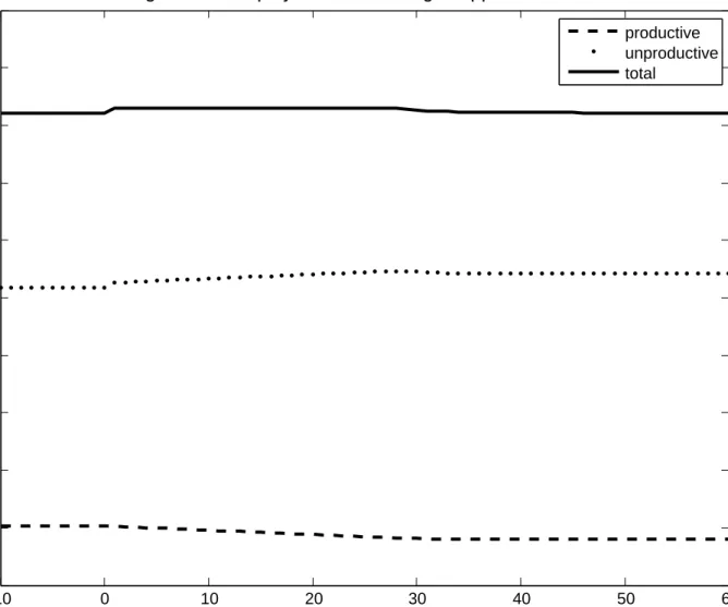
Figures 3.1 and 3.2 show the dynamics of the economy under wage suppression for a low level of domestic …nancial development = 0:15< 1. Under wage suppression, the wage

rate is so low that even the unproductive entrepreneurs enjoy a higher rate of return on production under autarky than the foreign interest rate. Thus both unproductive and productive entrepreneurs borrow from abroad. However, since the borrowing capacity is small, capital in‡ow is limited. The productive entrepreneurs also borrow from the unproductive entrepreneurs who become their lead creditors in the domestic credit mar-ket. Here, the unproductive entrepreneurs serve as …nancial intermediary: they borrow from the foreigners secured by the fraction of their output at the world interest rate

r , and, at the same time, extend loan to the productive entrepreneurs in the domestic credit market as the lead creditors at the domestic interest rate rt. The fact that the unproductive entrepreneurs act as …nancial intermediary stems from the fact that

in-ternational borrowing constraint is tighter than the domestic borrowing constraint (i.e.,

0< <1).17

The dynamics of the wage suppression economy is characterized by a temporary boom followed by stagnation. Immediately after the liberalization, the unproductive entrepreneurs expands production by borrowing from abroad at a cheaper interest rate. The total employment increases with capital in‡ow, which pushes up the wages. The expansion, however, is short-lived. Because the employment by the productive entrepre-neurs is crowded out with a higher wage, TFP keeps decreasing from autarky level. After the international borrowing constraint becomes binding, output and wage rate start de-creasing until the economy converges to its new steady state. The long-run e¤ect on output is marginal.

4.2

Interest Rate Suppression

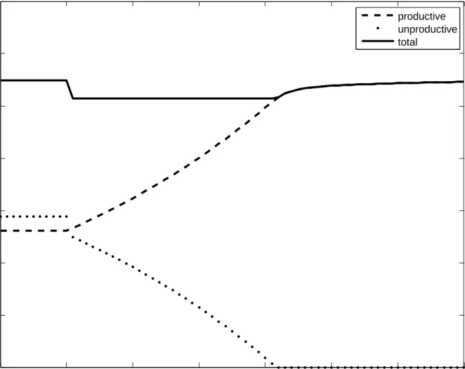
Figures 4.1 and 4.2 show the dynamics of the economy under the interest rate suppression for a medium level of domestic …nancial development = 0:3₂[ 1; 2]. The adjustment

process under the interest rate suppression is characterized by temporary drop in wages and employment followed by gradual expansion. Because the unproductive entrepre-neurs start lending abroad and reduce employment, wage and total employment drop immediately after liberalization. While total employment and employment of unpro-ductive entrepreneurs fall, employment of prounpro-ductive entrepreneurs rise due to cheap wage rate and borrowing rate. As a result, TFP improves. Over time, employment of productive entrepreneurs increases together with their accumulation of net worth, until

17_{During the rapid economic growth era after the World War II, Japanese general trading companies}

played a role of …nancial intermediary, borrowing from abroad against their international collateral and lending to domestic businesses. Possibly, countries like India and China (at least in the early stage) may experience this type of adjustment. Caballero and Krishnamurty (2001) has a similar feature.

it absorbs the entire employment. Thereafter, the wage rate and employment start re-covering. Intuitively the international capital market has a catalyst e¤ect by eliminating the ine¢ ciency in production in the long run through accumulation of net worth.18

4.3

Advanced Domestic Financial System

When domestic …nancial system is more advanced than the rest of the world, autarky interest rate is higher than the world interest rate due to large borrowing capacity of the productive entrepreneurs. After liberalization, the productive domestic entrepreneurs will attract foreign fund, causing capital in‡ow. The unproductive entrepreneurs con-tinue to specialize in lending. Figures 5.1 and 5.2 show the dynamics of the economy under advanced domestic …nancial system = 0:8> 2. The total employment (which

is equal to employment of the productive entrepreneurs) expands at the beginning and then stays roughly constant.19

Similar to the analysis by Caballero et al. (2006) and Mendoza et al. (2007) our framework suggests the existence of “equilibrium imbalances” in which countries with more developed …nancial system experience capital in‡ows as they integrate with less …nancially developed economies. Intuitively, the home economy can take advantage of the relatively low interest rate (and the saving glut) of the rest of the world. A distinguishing feature of our work is that capital in‡ow needs not be the result of superior domestic …nancial system, because it can be a result of wage suppression. But the key di¤erence among these two types of capital in‡ow is that TFP stays high with capital in‡ow induced by a superior …nancial system, while the TFP deteriorates and the boom is

18_{Perhaps, some Latin American countries experience this type of adjustment, which is characterized}

by capital out‡ow and the loss of employment of the unproductive sector, which may cultivate the anti-globalization sentiment.

19_{This depends on the elasticity of labour with respect to wage. If labour supply is elastic enough,}

temporary when capital in‡ow is caused by the wage suppression with an underdeveloped domestic …nancial system.

4.4

Steady State after Liberalization

The new steady state after capital account liberalization depends upon therelativelevel of domestic …nancial development to the rest of the world as:

Proposition 2 Letr( ) andw( ) be the domestic interest rate and the wage rate in the steady state equilibrium after liberalization with …nancial depth .

1. Wage suppression, < 1: Unproductive entrepreneurs produce and the home interest rate stays above the foreign interest rate: r < r( )< ra( ),w( ) > wa( ),

r0_{( ) <0 and w}0_{( )>0:}

2. Interest rate suppression, ₂[ 1; 2]: Unproductive entrepreneurs do not produce, and the home and foreign interest rates are equalized: ra_{( ) r( ) = r , A( ) =}

Aa_{( ), and w}0_{( )>0:}

3. Advanced domestic …nancial system, > 2: Unproductive entrepreneurs do not

produce. The home and foreign interest rates are equalized if 2 < e

+ [n +(1= r ) 1]

(1+n) +(1= r ) 1 2 ( 2;1): The home interest rate stays above the foreign interest rate if > e. In both cases, ra_{( ) > r( ), w( ) > w}a_{( ); A( ) = = A}a_{( ),}

r0_{( ) 0 and w}0_{( )>0:}

Note that unproductive entrepreneurs do not produce if the …nancial depth is at least as high as 1:Thus the economy is more likely to achieve e¢ ciency in production for the

account liberalization does not necessarily leads to the complete …nancial integration of the home economy with the rest of the world. If the …nancial depth of the economy is very di¤erent from the rest of the world, either extremely low < 1 or extremely high

>~; the domestic interest rate stays higher than the foreign interest rate because the international borrowing constraint is binding. From Proposition 2, we learn wage rate and total employment are increasing functions of the …nancial depth of the economy for the entire range of .

5

Welfare and Government Policies

5.1

Welfare Analysis

From the analysis of the previous section, we learn that the capital account liberalization is not necessarily bene…cial, especially when the domestic …nancial system is underdevel-oped. If the wage suppression is pronounced under …nancial autarky, the liberalization does not improve the TFP and thus the boom is temporary. If the interest rate sup-pression is signi…cant, the liberalization causes capital out‡ow and decline in wages and employment during the transition, even though the TFP will improve in the long-run. A natural question is to what extent capital account liberalization is bene…cial for the country, and how the costs and bene…ts are distributed among di¤erent groups. To answer this question, we examine the welfare e¤ects on workers and productive and un-productive entrepreneurs separately. (We do not use Pareto e¢ ciency criteria of whether everyone can be better o¤ with suitable redistribution, because it is di¢ cult to enforce redistribution with limited collateral).

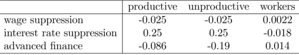
per-productive unproductive workers

wage suppression -0.025 -0.025 0.0022

interest rate suppression 0.25 0.25 -0.018

advanced …nance -0.086 -0.19 0.014

Table 1: Welfare analysis

centage change of steady state autarky consumption that is required to make an agent indi¤erent between liberalizing capital account and staying in autarky. In computing this measure, we take into account the e¤ects of the transition dynamics from autarky to the post-liberalization steady state. Formally, for each entrepreneursi, we de…ne this measure of welfare change - called the consumption equivalent i - as

E0 1 X t=0 t_{log c}i t = 1 1 log (1 + i_)cia ₍₃₅₎ whereci

tis datetconsumption of entrepreneuriafter the liberalization at date0, starting from the autarky steady state at date 1, and cia _{is his consumption under autarky} steady state.

The welfare measure of workers is de…ned in a similar way. Assume that the utility of the workers is logarithmic: u(c v(l)) = log(c v(l))and that the disutility of labor is constantly elastic: v(l) = 1 1+(1= )l 1+(1= )_{. De…ne} w _as 1 X t=0 t_{log (c} t v(lt)) = 1 1 [logc a_{(1 +} w_{) v(l}a_{)]; (36)}

where w is consumption equivalent for the workers. Here ca and la respectively denote consumption and labor supply under autarky.

Table 1 reports the welfare e¤ect of capital account liberalization for the cases corre-sponding to wage suppression, interest rate suppression and advanced domestic …nancial

system, using the numerical example of the previous section. The headline of ‘produc-tive’ implies the group of entrepreneurs who are productive and ‘unproduc‘produc-tive’ is the group who is unproductive at the time of liberalization. Under wage suppression, capital in‡ow is limited and boom is temporary because the borrowing constraint is tight and as a result the welfare e¤ects of liberalization are small compared to the other two cases. The workers gain only modestly from the temporary boom and the entrepreneurs lose modestly from the lower expected rates of return.

Under interest-rate suppression, the economy experiences an initial recession before improving the TFP in the long-run. The workers tend to lose since the loss from the lower wages during the initial recession is large compared to the possible long-run gains in a distant future. The entrepreneurs gain substantially because their rate of return become higher. The unproductive (savers) obtain better saving opportunities abroad at the higher world interest rate, and the productive entrepreneurs achieve higher rate of return due to lower wages. The welfare e¤ects on the entrepreneurs are much larger than those on workers since changes in the rate of return have compound e¤ects on their consumption through wealth accumulation.

Finally, in the case of advanced …nancial system, the workers gain due to perma-nently higher wages. The entrepreneurs lose because they face lower rate of return. In particular, unproductive entrepreneurs loose substantially because they are savers at the time of liberalization and their rate of return on saving drops to the world interest rate. In contrast, productive entrepreneurs do not loose as much because they can expand production by borrowing at a cheaper world interest rate even though the wage rate is higher.

From these analysis, we learn that there tends to be con‡icts of interests between workers and entrepreneurs towards the capital account liberalization. The welfare of the

workers tend to be more in‡uenced by the short-run movement of the aggregate economy immediately after the liberalization, because the workers do not smooth consumption due to the binding borrowing constraint. In contrast, the entrepreneurs tend to care more about the subsequent rates of return which depends upon the long-run performance of the economy.

From a policy maker’s point of view, the case of interest-rate suppression would be of particular interest. This is because capital account liberalization of private capital ‡ows can eventually eliminate the ine¢ ciency of production, but such process can be painful to the workers who su¤er from lower wage and employment. Can the government mitigate the loss of workers during the adjustment to the capital liberalization? One possibility is redistribution, but the government may face a limited enforcement problem similar to that of the private agents as long as the domestic …nancial and legal systems are not developed enough. Therefore, in the next two Sections we consider two di¤erent types of policy intervention. The …rst one is a simple tax and subsidy policy under balanced budget constraint, while the second one is to allow foreign direct investment (FDI) ‡ows along with private capital ‡ows in the process of capital account liberalization.

5.2

Tax and Subsidy under Interest Rate Suppression

The reason for which wages drop temporarily under interest-rate suppression is that the unproductive entrepreneurs lend abroad and shrink their production. In order to mitigate the drop in wages, we consider a production subsidy to unproductive agents by imposing taxes on the productive agents. We assume balanced budget, so the budget constraint of the government sector is given by

where t represents subsidy rate and t represents tax rate.20

Limited commitment and shortage of collateral have implications for both private …nance and public …nance. Because the tax liability to the government is considered to be the most senior debt of the entrepreneur, it a¤ects his domestic and international borrowing constraints as

tyt+1+bt+1 yt+1; (38)

tyt+1+bt+1+bt+1 yt+1: (39)

The …rst constraint implies that the foreign creditors will limit their loans so that the sum of the tax liability and the foreign debt repayment does not exceed the value of collateral for the outside creditors. The second constraint says the domestic lead creditor restricts her loan so that the sum of all liabilities of the entrepreneur does not exceed the collateral value of the project to the lead creditor. In what follows, we assume that the tax liability of the entrepreneur does not exceed the collateral value for the outside creditors: tyt+1 yt+1.21 The ‡ow-of-fund constraint of the productive entrepreneur

becomes ct+wtlt= (1 t 1)yt bt bt + bt+1 rt + bt+1 r (40)

The unproductive entrepreneur’s ‡ow-of-fund constraint is similar to (40), term t 1

being replaced by t 1.22 In Appendix D we describe the set of equilibrium conditions.

20_{The role of public debt as liquidity in an economy under credit constraint is an interesting question.}

For example, Woodford (1990) considers a model with heterogeneous entrepreneurs who cannot borrow, in order to argue that government can issue public debt to absorb the saving of the unproductive entrepreneurs and improve the e¢ ciency. See, also, Holmstrom and Tirole (1997). However, a systematic analysis of public debt under credit-constrained economy is beyond the scope of this paper and is left for future research.

21_{This constraint can be an outcome of limited power of government who cannot enforce tax liability}

more than the outside creditors.

22_{We assume that the unproductive entrepreneur who receive production subsidy cannot borrow}

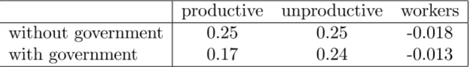
productive unproductive workers without government 0.25 0.25 -0.018

with government 0.17 0.24 -0.013

Table 2: Welfare with government under interest-rate suppression

F igure 6 shows the dynamics of the economy with government under interest-rate

suppression. Here, subsidy is chosen to set the wage immediately after liberalization as

wt= wa+ (1 )wtl;

where wa _{is wage under autarky steady state and w}l

t =r is wage immediately after liberalization without government policy. Here is set 0.3. There is a trade-o¤ for our government policy. On one hand, the unproductive entrepreneurs who receive sub-sidy employ more workers than the laissez faire economy during transition. As a result employment is larger with the government policy. On the other hand, taxation on the productive entrepreneurs decrease their capacity of private borrowing. As a result their accumulation of net worth and expansion of employment are slower. Thus the transition to the equilibrium with e¢ cient production takes longer than the laissez faire econ-omy.23 _{Eventually, the unproductive entrepreneurs stop producing, and thereafter the}

adjustment is identical to the laissez faire economy. Table 2 shows welfare consequences of the government policy. Not surprisingly, workers’loss is mitigated. The productive entrepreneur’s gain from liberalization shrinks by the taxation. The unproductive en-trepreneur’s gain does not change much, because their rate of return is still given by the foreign interest rate despite of receiving the production subsidy.

the production subsidy from the government.

23_{If subsidy is large enough to maintain the autarky wage, the employment of the productive}

entrepre-neurs starts shrinking as their net worth deccumulates. Then the tax rate on output of the productive agents have to be higher in order to balance the budget, which leads to further deccumulation of their net worth. Thus, the large subsidy program is not sustainable in the long run.

5.3

Foreign Direct Investment

Another policy intervention which has become increasingly more important is to allow foreign direct investment (FDI) along with …nancial capital ‡ows.24 Allowing FDI might imply smaller distortion than the tax and subsidy policy of the previous section. Also, it has been argued that FDI tends to be the least volatile type of capital ‡ows because it involves relatively irreversible types of investment (physical capital, human capital, managerial resources)25_{. Therefore allowing FDI may make countries less vulnerable to}

capital out‡ow. In this section we are interested in examining whether the FDI is able to mitigate the losses of workers in the interest rate suppression region.26

We assume that foreign …rms have a similar production technology as domestic en-trepreneurs:

yt+1 = lt; (41)

where yt+1 is output of goods at date t+ 1, lt is the labor input at date t, and is constant productivity of foreign …rms. Here we assume that foreign productivity is at least as big as the productivity level of the productive entrepreneurs, . Since we consider a small open economy, when foreigners make their decisions about FDI they

24_{As documented recently in Prasad and Rajan (2008), the share of foreign direct investment ‡ows}

has now become far more important than that of debt in gross private capital ‡ows to nonindustrial countries. The share of foreign direct investment in total gross in‡ows to emerging markets and other developing countries has risen from about 25 percent in 1990-94 to nearly 50 percent by 2000-04. Over the same period, the share of debt in in‡ows to emerging markets has fallen from 64 percent to 39 percent.

25_{Kose et al. (2006) looks at the volatility of di¤erent types of in‡ows, calculated as the cross-country}

averages of the standard deviations of di¤erent types of in‡ows (measured as ratios to GDP) over the period 1985-2004. They …nd that gross in‡ows of debt …nancing are substantially more volatile than FDI or equity in‡ows.

26_{A important issue in FDI is technology transfer (see for example Blalock and Gertler (2008) for the}

case of Indonesian manufacturing establishment). While it is certainly an important issue we abstract from it because our main focus in the paper is to explore how liberalization of international …nancial transactions a¤ect resource allocation among heterogeneous producers subject to credit constraints. We believe we can analyze the role of FDI in this regard without considering the spillover e¤ects.

are not subject to borrowing constraints. Therefore the relevant discount factor is the international interest rate r :

On the other hand, it seems natural to assume that foreign producers face frictions in expanding production: In particular, it takes time and cost for the foreign employers to recruit suitable workers who understand technology and organization of the …rm. We capture this by search frictions along the line of Mortensen and Pissarides (1994). In order to hire a suitable worker, a foreign employer maintains an open vacancy at ‡ow cost c. A ‡ow of new worker-employer matches is given by a constant-returns-to-scale function M(Ht; Vt), where Ht is the number of searching workers andVt is the number of vacancies in the economy. Here we assume that all the workers (including the workers employed by the domestic …rms) can costlessy look for jobs in foreign …rms. Then given the constant population of workers, Ht is constant. For simplicity, we assume that workers can supply labor to domestic and foreign …rms simultaneously, and that each worker supplies one unit of labor when they match with foreign producers, so that foreign …rms have only extensive margin to adjust labor. Finally, the relationship between foreign …rm and a worker might end every period with a exogenous separation rate 1 .

Total labor force in the FDI sector (Pl_t =L_t) evolves according to

L_t = L_{t 1}+M(H; Vt); (42)

where the …rst term represents the fraction of employed workers who remain employed in foreign …rms and the second component represents workers who …nd a job. The

matching function is given by

M(H; Vt) = ~H Vt1 = V

1

t : (43)

The model is completed by the relationship that determines the link between the value of the vacancy and the value of the job. The recursive equation for the value of the vacancy is given by

J_tv = c+ V_t Jt+ (1 V_t ) r J v t+1; (44) where Jv

t is the value of the vacancy, Vt represents the rate at which the vacancy is …lled and Jt is the value of the job that evolves accordingly to

Jt=

r wt+r Jt+1: (45)

In (45), the term _r wt represents the current net bene…t from the match while the last term represents the continuation value which depends on the separation rate. We assume free entry, implying that J_tv = 0 at all times. In contrast to the production by the foreign …rms, we continue to assume that all the workers are homogeneous and suitable for the production by the domestic entrepreneurs. Assuming that the foreign …rms have full bargaining power against the workers, the foreigners will choose the wage equal to the competitive wage level.

The competitive equilibrium condition in the labor market is now

Lt+L0t+Lt =L

s_(w

Once we use (42), (43) and (44) to substitute out the measure of vacancies, Vt; the dynamic evolution of the economy is characterized by the recursive equilibrium:

Zt+1; st+1; xt; rt; wt; Lt; L

0

t; Lt; Bt+1; Jt that satis…es (16), (17), (21 - 25), (42), (45), and (46) as functions of the state variables(st; Zt; Lt 1):

In the subsequent analysis we focus on the adjustment in the case of interest-rate suppression when the economy starts from its steady state without international …nancial transactions but with FDI allowed. Then the economy liberalizes the international …nancial transaction with the continued presence of FDI. This exercise seems to be useful for thinking about the experience of some countries, such as China, which is allowing FDI while keeping strict restrictions on international …nancial capital ‡ows.

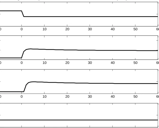
F igure7shows how the presence of the FDI changes the adjustment of the …nancially

suppressed economy to the liberalization of international …nancial transactions. The parameter values used are discussed in Appendix. Solid line and uneven dotted line plot the dynamic path with FDI. For comparison, even dotted lines plot the adjustment of the economy without FDI — identical to Figure 4.2. Prior to liberalization of international …nancial transaction with the presence of the FDI, employment of the unproductive domestic entrepreneurs is smaller and the TFP is higher than the steady state without the FDI, because a fraction of workers are employed by productive foreign …rms.27

Immediately after the liberalization of international …nancial transaction, wages fall as much as the case without the presence of FDI. This is because, as long as the un-productive entrepreneurs still produce, the unun-productive agents are indi¤erent between producing and lending abroad: =wt = r . However, because employment of foreign

27_{Because of our speci…c feature of the domestic entrepreneurial sector (such as constant returns to}

scale production function, constant turnover rate, and constant saving rate), the FDI does not change the share of wealth and employment of the productive entrepreneurs within the domestic entrepreneurial sector. Thus the wage rate, total employment and domestic interest rate are not a¤ected by the FDI in the steady state under …nancial autarky.

productive unproductive workers without FDI 0.2533 0.2533 -0.01815

with FDI 0.2532 0.2532 -0.01807

Table 3: Welfare with FDI under interest-rate suppression

…rms expands in addition to that of productive entrepreneurs, it takes less time for the unproductive production to be eliminated and the wage level recovers more quickly.28

Table 3 reports the welfare e¤ect of capital account liberalization with and without FDI. Qualitatively, we see that by shortening the initial recession FDI mitigates the workers’s loss. However under our chosen parameter values the e¤ect is very small.29

The presence of FDI does not have much e¤ect on the welfare of entrepreneurs either since their rate of return is not directly a¤ected by the presence of FDI. Overall, by making domestic entrepreneurial employment smaller, the presence of FDI speeds up the necessary adjustment to the liberalization of the international …nancial transactions. However, the prices and the distributions among the domestic sectors in the new steady state are mostly determined by the domestic institution, not directly a¤ected by the FDI in our framework in which there is no direct spillover e¤ects from the FDI to the domestic technology and institution.

28_{At the new steady state again, the presence of the FDI does not a¤ect the distribution of wealth}

and employment between productive and unproductive domestic entrepreneurs, and thus does not a¤ect wage rate and total employment.

29_{The share of FDI in the initial period (i.e., at the time of liberalization) is important in determining}

the quantitative signi…cance of the welfare e¤ect on workers. As is explained in Appendix E we chose the parameter values such that the share of FDI is about 20%. If the share of FDI is higher, it takes less time for the unproductive production to be eliminated, and the resulting welfare gain is higher.

6

Final Remarks

We have developed a model of capital account liberalization under domestic and inter-national borrowing constraints in which workers and entrepreneurs might not bene…t from …nancial integration as long as the domestic …nancial system is underdeveloped. If wage suppression is dominant with underdeveloped domestic …nancial system, then the liberalization leads to a deterioration of TFP and long-run stagnation. If interest rate suppression is more pronounced, then the liberalization causes capital out‡ow and signi…cant loss of employment during the adjustment. The reason for which capital ac-count liberalization generates these costly adjustments is because under underdeveloped …nancial system funds are used by unproductive entrepreneurs and producers located in foreign countries rather than productive domestic entrepreneurs.

Our logic might extend to …nancial liberalization across regions or di¤erent segments of the economy. For example, Guiso, Sapienza and Zingales (2004) …nd that the regions with better local …nancial system in Italy enjoy better economic performance after the …nancial liberalization of the mid-1980s as they have more entries of new …rms, smaller monopoly markup, and higher growth.30

Of course, an important remained question would be to examine how to improve the domestic …nancial system.

30_{Reinhart and Rogo¤ (2008) argue that the subprime mortgages could be interpreted as lending to}

developing countries, because those loans are directed to the "under-developed" segment of the U.S economy. Then, the …nancial liberalization of this segment may fail to improve the resource allocation in the long-run unless the …nancial system within this segment is improved..

Appendix

A

Proof of Proposition 1:

From(27) and (28); we learn there are three possible types of the equilibrium: (i) Unproductive entrepreneurs produce (L0 _{>0; r=}

w)

(ii) Unproductive entrepreneurs do not produce and productive entrepreneurs are credit constrained(r _{2 w};_w )

(iii) Unproductive entrepreneurs do not produce and none is credit constrained

r = _w

Let us now examine each type of equilibrium in turn in order to derive the necessary and su¢ cient condition on the parameters for such equilibrium to exist.

A.1

Autarky equilibrium with ine¢ cient production:

Because the interest rate is less than the rate of return of production on productive entrepreneurs:

r=

w < w; (A.1)

the productive entrepreneurs are credit constrained. (28) becomes:

L= X

( =r) w Z =

X

Z: (A.2)

For employment of unproductive entrepreneurs to be positive, we need from goods mar-ket equilibrium condition(30) that:

X < : (A.3) From(31) and (A:1);we learn x= ( )=( ): Thus, from (33); X solves

F(X; ) =X[X+ (1 +n)] [(1 )X+n ] = 0: (A.4)

Because F(0; )<0; we knowX >0;which implies from (32) that

r= 1

(1 +X) < 1

:

Thus, we verify the condition (13) that guarantees that workers do not save in the neighborhood of the steady state equilibrium. Also, we learn the condition for ine¢ cient production(A:3) holds if and only if; F( ; )>0; or

<

+ (1 +n) : (A.5)

From(A:4); X and w are increasing functions of ;and r is a decreasing function of .

A.2

Autarky equilibrium with e¢ cient production and credit

constrained productive entrepreneurs:

Here, because there is no employment by the unproductive entrepreneurs (L0 = 0) and the productive entrepreneurs are credit constrained, the equilibrium conditions (28)

-(30) imply Ls= Z w =L= X Z ( =r) w; and w= (1 +X)r = :

Together with (31) -(33), we learn

X = 1 (1 +n) : (A.6)

Then, we learn the productive entrepreneurs earn extra return X > 0 so that they are credit constrained, if and only if

< 1

1 +n:

Also we learnr = 1=[ (1 +X)]<1= , which veri…es(13).

A.3

Autarky equilibrium in which no one is constrained:

If, 1=(1 +n); then we learn

X = 0; r = 1= ; w= ; and s= n

1 +n

satisfy all the equilibrium conditions of the steady state autarky equilibrium in which none of the entrepreneurs are credit constrained. (See footnote 13). Concerning the quantities, we haveL0 _{= 0 and:}

L=Ls( ) =Z= :

B

Proof of Proposition 2

From the generic equilibrium conditions, (16) - (18) and (21) - (25), the steady state equilibrium of the open economy is characterized by (r; w; x; X; L; L0_{; Z) that satis…es} the conditions (29), (32), (33) and

r (1 ) w ( =r ); and r (1 ) w ( =r ) L 0 _{= 0; (B.7)} L= XZ ( =r) w+ [(1=r ) (1=r)]; (B.8) Z+ r [ L s_{(w) + ( )L] wL}s_{(w); and (B.9)} (r r ) Z+ r [ L s (w) + ( )L] wLs(w) = 0; x= wr+ r r r wr r r_r : (B.10)

B.1

Wage suppression:

<

Proof. Suppose not. Then, from(8), we learn r=r : Then we have

ra > r =r; for < 1;

by construction of 1. Then, from(32);we learn

Then from(33), we obtain xa = < x= wr wr ; or r < w < (1 ) w =r : This contradicts(B:7).

Guess L0 >0 in(B:7). ThenLemma 3 implies

r = (1 ) w ( =r ); or w = r + 1 r = [1 +X+ (X X)]: (B.11)

where 1 +X = 1= r : Then from(B:10); we learn

x= ( ) 1 + X X 1+X ( ) X X 1+X :

Thus from (33), we have

e

F(X; ; ) X[X+ (1 +n)] [(1 )X+n + (X X)(X+n )] = 0:

Then we see X0( ) > 0, or r0( ) < 0. Also because Fe(X; ; ) < F(X; ) for

X ₂ (0; X ); we learn X > Xa, or r( ) < ra( ). Then from (B:11) and Proposition 1, we learn w( ) > wa_{( ). We can also verify that L}0 _{> 0 from (B.8) and (B.9) under} Lemma 3.

B.2

Interest rate suppression:

2

[

;

]

1; 2)

Proof. By de…nition of ( 1; 2); we know r( ) r > ra( ) for 2 ( 1; 2). Thus

X < Xa, or x= wr+ r r 1 wr r r 1 < xa = w a_ra wa_ra : Thus < wr _rr 1 ; or w > r + 1 r 1 r > 1 r + r :

Thus from (17); we learn L0 _{= 0 for 2(}

1; 2).

Lemma 5 r =r for ₂( 1; 2)

Proof. Suppose that r > r : Then from Lemma 4, (B:8) and (B:9), we learn

w r L = Z = 1 X r w+ 1 r 1 r L; or w = (1 + X ) Then, x=X 1 1 (1 )X:

Also from (33), we know

x=X X+ (1 +n)

Therefore we learn

0 = (1 ) [(