Machine learning and option implied information

(1)

Imperial College London

Doctoral Thesis

Machine Learning and Option

Implied Information

Author:

Yu Zheng

Supervisor:

Prof. Michaelides

Alexander

A thesis submitted in fulfillment of the requirements

for the degree of Doctor of Philosophy

in the

Finance Department

Imperial College Business School

(2)

Declaration of Originality

I, Yu Zheng, declare that this thesis titled, Machine Learning and Option Implied Information, and the work presented are my own. I confirm that:

• This work was done wholly or mainly while in candidature for a research degree at this University.

• Where any part of this thesis has previously been submitted for a degree or any other qualification at this University or any other in-stitution, this has been clearly stated.

• Where I have consulted the published work of others, this is always clearly attributed.

• Where I have quoted from the work of others, the source is always given. With the exception of such quotations, this thesis is entirely my own work.

• I have acknowledged all main sources of help.

• Where the thesis is based on work done by myself jointly with others, I have made clear exactly what was done by others and what I have contributed myself.

Signed: Yu Zheng

(3)

Copyright Declaration

The copyright of this thesis rests with the author and is made available under a Creative Commons Attribution Non-Commercial No Derivatives licence. Researchers are free to copy, distribute or transmit the thesis on the condition that they attribute it, that they do not use it for commercial purposes and that they do not alter, transform or build upon it. For any reuse or redistribution, researchers must make clear to others the licence terms of this work

(4)

Acknowledgement

Firstly, I would like to express my sincere gratitude to my advisor Prof. Michaelides Alexander for the continuous support of my Ph.D study and related research, for his patience, motivation, and immense knowledge. His guidance helped me in all the time of research and writing of this thesis. I could not have imagined having a better advisor and mentor for my Ph.D study.

Besides my advisor, I would like to thank the rest of my thesis commit-tee: Prof. Kacperczyk Marcin, Dr. Julliard Christian, for their insightful comments and encouragement, but also for the hard question which in-cented me to widen my research from various perspectives.

I thank my friends Ran Fan and Yongxin Yang for the stimulating dis-cussions, for the sleepless nights we were working together before deadlines, and for all the fun we have had in the last four years.

Last but not the least, I would like to thank my family: my parents and my wife for supporting me spiritually throughout writing this thesis and my life in general.

(5)

Abstract

The thesis consists of three chapters which focus on two broad topics, applying machine learning in finance (Chapters 1 and 2) and extracting implied information from options (Chapter 3).

In Chapter 1, I combine the data-driven approach from the machine learning community and economic theory from the finance community to design a deep neural network to estimate the implied volatility surface.

Chapter 2 is a second example of applying machine learning in finance. Yang et al. [2017] proposes a gated neural network for pricing European call options. Yang et al. [2017] is rewritten in this chapter using the general framework introduced in Chapter 1.

In Chapter 3, I provide a solution to the following question. Is there any flexible implementation framework to derive the conditional risk neu-tral density of any arbitrary period of return and calculate corresponding statistics, namely, implied variance, implied skewness and implied kurtosis from option prices? I solve this problem by proposing a framework com-bining implied volatility surface and Automatic Di↵erentiation [Rall, 1981, Neidinger, 2010, Griewank and Walther, 2008, Baydin et al., 2015].

(6)

Introduction

The thesis consists of three chapters which focus on two broad topics, applying machine learning in finance (Chapters 1 and 2) and extracting implied information from options (Chapter 3).

In Chapter 1, I combine the data-driven approach from the machine learning community and economic theory from the finance community to design a deep neural network to estimate the implied volatility surface. I propose a framework on how to design a deep learning network combined with economic assumptions. This approach can be used for any modelling purpose rather than just modelling the implied volatility surface. The empirical experiments show that our model has better performance, in-sample and out-of-in-sample, than the benchmark model.

Chapter 2 is a second example of applying machine learning in finance. Yang et al. [2017] proposes a gated neural network for pricing European call options. They integrate assumptions of a valid call option surface from classical mathematical finance literature into neural network as inductive bias. Yang et al. [2017] is rewritten in this chapter using the general frame-work introduced in Chapter 1. The neural netframe-work model outperforms ex-isting learning-based and some mathematical finance models, and comes with guarantees about the economic rationality of its outputs.

In Chapter 3, I provide a solution to the following question. Is there any flexible implementation framework to derive the conditional risk neu-tral density of any arbitrary period of return and calculate corresponding statistics, namely, implied variance, implied skewness and implied kurtosis from option prices? I solve this problem by proposing a framework com-bining implied volatility surface and Automatic Di↵erentiation [Rall, 1981, Neidinger, 2010, Griewank and Walther, 2008, Baydin et al., 2015]. The

(9)

• It is flexible to change the implied volatility surface model without changing the main programming code. This is achieved by intro-ducing Automatic Di↵erentiation. Construction of an arbitrage-free implied volatility surface is a well-studied research area and new mod-els are still coming out. Switching between these modmod-els to select the best one is clearly an advantage.

• The conditional risk neutral density of arbitrary period of return, for example, weekly, monthly or quarterly, can be derived from the framework on each trading day. Furthermore, daily time series of implied variance, skewness and kurtosis with respect to the return distribution is readily computed.

With the help of the above framework to construct the implied informa-tion, I test the hypothesis whether predictability of variance risk premium on S&P500 index return still holds for shorter frequency, say weekly, bi-weekly or tribi-weekly. This question will be of interest to practitioners as if the predictability exists, short term trading strategy can be designed. Furthermore, if the predictability exits, this will be an example demon-strating that the short term options, which are ignored by academic are worth studying [Andersen et al., 2017]. Furthermore, I also explore an interesting question as to whether di↵erent weekdays, which are used to define weekly return and weekly variance risk premium, will influence the predictive power.

From the regression results, we conclude that the weekly frequency re-sults are more informative than biweekly and triweekly as only Wednesday is not significant if the alpha level is 5%. For biweekly and triweekly re-sults, only two out of five days are significant and these weekdays are not the same. This raises an interesting question as to whether there exists a weekday e↵ect which influences the predictive power of the short-term variance risk premium. The monthly and quarterly results are consistent with the literature [Bollerslev et al., 2009, Carr and Wu, 2009, Bollerslev et al., 2011, Bondarenko, 2014, Xiao and Zhou, 2015]. This analysis allows us to conclude that the framework is useful in constructing the implied information for prediction purposes.

(10)

Chapter 1

Neural Network for Implied

Volatility Surface: Bayesian

alike Design Approach

1.1

Introduction

The implied volatility surface (IVS) is one of the most important con-cepts in mathematical finance. The implied volatility is defined as the inverse problem of option pricing, mapping from the current market price to a single number, which is the volatility parameter of the underlying process in the Black-Scholes model [Black and Scholes, 1973a]. Although the assumptions in the Black-Scholes model can be criticised due to the fact that real-world distributions are often fat-tailed and asymmetric, the Black-Scholes formula is still popular in industry as it provides a conve-nient mapping from the price space to the implied volatility space. When the variation of implied volatility is plotted against option strikes and time to maturity, it is referred to as the implied volatility surface.

The implied volatility surface is widely studied by academics and practi-tioners. For any fixed time instance, one can observe a non-flat IVS which is contrary to the constant volatility assumption in the Black-Scholes model. If we fix the time to maturity, the implied volatility slice exhibits skew or smile pattern which results from the non-normality of the conditional

(11)

the IVS provides the information about the term structure of the implied volatility at that particular strike. The combination of skew or smile and the term structure of implied volatility on the IVS reveals how the condi-tional risk neutral density of the underlying return varies across strikes and time to maturity. Furthermore, the level and shape of IVS are changing every day [Cont and Da Fonseca, 2002] which also provide the evolution of conditional risk neutral density of underlying return. These features of the IVS inspire academics to model the IVS directly rather than the option prices.

Modelling the IVS may not be as easy as it looks as the constructed IVS may not be arbitrage free. This will cause problems for practitioners. Market makers need an arbitrage-free IVS to provide quotes for illiquid or not listed options. Pricing models for exotic options are usually calibrated against a valid IVS. To calculate the risk profile of an option portfolio, a valid IVS needs to be constructed to define the loss events.

To solve the above problems, a great deal of literature is devoted toward constructing an arbitrage-free IVS. Homescu [2011] provides a complete review on methodologies for constructing the IVS. There are mainly two groups of methods. The first group is an indirect method in the sense that IVS is derived from other models rather than modelled explicitly. It in-cludes local volatility models, stochastic volatility models and levy models [Heston, 1993a, Merton, 1976, Kou, 2002] The main problem for this group is that models normally dont have a sufficient number of parameters to fit the market data. Although time dependent parameters can be introduced, this will lead to much difficulty with regard to computational time and optimisation. The second group is called a direct method because the IVS is explicitly specified. In direct methods, there are two distinct ways for modelling the IVS. The first approach specifies the dynamics of the IVS and assumes it evolves continuously over time [Carr and Wu, 2010]. The second approach pays attention to the static representation of the IVS, either parametric or non-parametric.

The static representation of the IVS attracts the attention of many researchers. These methods do not consider the evolution of the under-lying like stochastic volatility models but find some parametric or non-parametric models to fit the implied volatility surface. As the implied

(12)

volatility surface is modelled directly, these methods normally have better quality in terms of fitting the market data than stochastic volatility models. They do not tell us anything about the dynamics of the implied volatil-ity surface. However, they do provide a snapshot of the current market situation.

One of the most popular methods in industry, the stochastic-volatility-inspired (SVI) model, is proposed by Gatheral [2004] to model the implied volatility slice for a fixed time to maturity. Gatheral and Jacquier [2014] updates the model SVI [Gatheral, 2004] to surface SVI (SSVI). It has sim-ple representations than SVI in terms of conditions for no static arbitrage. Kotz et al. [2013] construct an arbitrage-free implied volatility surface by introducing a quadratic deterministic volatility function. The arbitrage conditions are forced through two minimisation problems related to the volatility function.

Corlay [2013] employ B-splines to construct an arbitrage-free implied volatility surface and a new calibration method is proposed for sparse op-tion data. Itkin [2015] proposes a non-parametric method to model the implied volatility surface using polynomials of sigmoid functions. However, arbitrage-free conditions are held only at the nodes of discrete strike-expiry space.

Although there are many di↵erent approaches to model the IVS, they come mainly from mathematical finance or finance literature. This paper, instead, models the IVS using deep learning inspired from the machine learning literature. Deep learning is a re-branding of neural networks. In this paper, these two names are interchangeable. One motivation for picking up deep learning to solve the IVS problem is the observation that increasing number of quotes are available from exchanges (see Figures 1.4 and 1.5). It might be interesting to find a straightforward model to increase the model capacity (number of parameters) to cope with the growing num-ber of data. This will be more convincing if high frequency option data is available. Second, the advance of computer technology, especially parallel computing on CPUs and GPUs, and availability of new optimization al-gorithms make deep learning applicable (eg fitting quickly and efficiently) and very popular these days. Therefore, both facts make it worth revisiting

(13)

are 5116 trading days. On each trading day, we train a IVS using deep learning. This requires a huge amount of computation. It might run more than one month if it is done on a single pc even with parallel programming on GPU. We employ the HPC (High Performance Computing) provided by Imperial College London and make this research possible and get the result in a day.

Recently, we have seen machine learning is becoming increasingly pop-ular. It is mainly served as a method for complex pattern recognition from a large amount of data or making intelligent decisions based on big data. It includes three main categories, supervised learning, unsupervised learn-ing and reinforcement learnlearn-ing [Hastie et al., 2001, Bishop, 2006, Barber, 2012, Murphy, 2012]. Extensively implemented in a large variety of do-mains such as biology and computer science, machine learning can also be employed to solve finance problems.

Gavrishchaka [2006] proposes a boosting-based framework for volatil-ity forecasting. He uses boosting, a method of ensemble learning, to train a collection of the generalised autoregressive conditional heteroskedastic-ity (GARCH) models. Audrino and Colangelo [2010] present a semi-parametric method for implied volatility surface, the base model of this work is the regression tree, and they try to sequentially minimize the dif-ference between model prediction and ground truth via adding more trees. Coleman et al. [2013] use kernel machine to calibrate the volatility func-tion for opfunc-tion pricing. They train a support vector machine with spline kernel function, and the coefficient is regularised by `1 norm to encourage

sparsity. One drawback of those methods is that they just evaluate their algorithms on a relatively small dataset, e.g., [Gavrishchaka, 2006] targets on IBM stock option only, and [Audrino and Colangelo, 2010, Coleman et al., 2013] evaluate their approach on a short period (one month) of S&P 500 index option.

Machine learning techniques have many benefits such as being appli-cable to large data set, usually fast and relatively easy implementation in practice. However, the philosophy of machine learning techniques are much di↵erent from models in finance literature. Models in finance literature are usually based on certain economic theories (e.g., no arbitrage theory). These assumptions serve as a guideline and models are designed through

(14)

these assumptions. The problem with this approach is that assumptions might be too restrictive (e.g., a variable follows a Brownian Motion) and the number of parameters of the models is usually fixed. An increas-ing amount of data will make optimisation difficult. In contrast, machine learning solves problems in a data-driven way. The complicated relation-ship between model input and output is learned from a large amount of data rather than specified by economic results. This approach also exhibits some problems. First, it completely ignores economic results with respect to the modelling problem. Second, insufficient data coverage of the domain of interest might lead to unreliable results.

However, there is the possibility of combining the data-driven approach from the machine learning community and economic theory from the fi-nance community to design a deep neural network to estimate the IVS. The idea of the combination approach has been explored by Yang et al. [2017] who propose a gated neural network for pricing European call op-tions. They integrate assumptions of a valid call option surface from clas-sical mathematical finance literature into neural network as inductive bias. The idea of inductive bias is similar to the prior knowledge concept in Bayesian statistics.

Our contribution to the literature is as follows. First, we propose a framework on how to design a deep learning network combined with eco-nomic assumptions. This approach can be used for any modelling pur-pose rather than just modelling the IVS. Second, our deep learning model has better performance, in-sample and out-of-sample, than the benchmark model SSVI. Third, there is still plenty of room to boost the deep learn-ing models by investigatlearn-ing the model hyper-parameters. Fourth, the deep learning model has the potential to be used in high-frequency option data. Last, there is little research available on how to combine machine learning and finance in a coherent way to solve modelling problems; we hope we give some hints on how to explore this research area.

This paper is organised in the following way. In section 3.3, we will first give an introduction to neural network. Then we provide two useful techniques which can help to encode constraints in financial modelling into the design of deep learning networks. These techniques are illustrated by

(15)

for the IVS modelling problem. We propose a framework, called Bayesian-like design approach, to guide how to design deep learning network to solve financial modelling problems. In section 1.4, we follow the Bayesian-like design approach to design our deep learning network to solve the IVS modelling problem. We list the prior information and shows how the prior information is encoded into the design of deep learning network. In section 1.5, we train the prior deep learning models and compare them to other benchmark models.

1.2

Background

1.2.1

Introduction to Neural Network

Neural Networks Schmidhuber [2015], recently re-branded as deep learning Lecun et al. [2015], is a very popular algorithm in machine learning.

A key property of neural network is that, given appropriate parameters, it can approximate any continuous functions. This is known as universal approximation theorem Cybenko [1989], Hornik [1991].

The simplest neural network model contains two layer: an input layer where the data flows in, and an output layer where the predictions are produced. Assuming that the input data is ofN-dimension, and the output is of M-dimension, the two-layer neural network can be formulated as,

ˆ

y =xTW +b (1.1)

Here W is a matrix of size N _⇥M and b is a vector of length M. In the literature of neural network, W is usually referred to as weight term, and b as bias term.

Denote the set of parameters as ⇥ where ⇥ = {W, b}, the process of training or learning a neural network model (a.k.a. parameter estimation) is to solve the following optimisation problem,

argmin ⇥ 1 N N X n=1 `(yn,yˆn) = argmin W,b 1 N N X n=1 `(yn, xTnW +b) (1.2)

(16)

`y,yˆ is a loss function that measures the di↵erence between ground-truth outputy and the predicted output ˆy, e.g.,`(y,y) = (yˆ y)ˆ 2 _{calculates the}

squared di↵erence of two values.

The advanced neural network models are di↵erent with Eq. 1.1 by two factors: (i) hidden layer (ii) activation function.

A hidden layer is one extra degree of computation, e.g., a three-layer neural network can be written as,

ˆ

y = (xTW¯ + ¯b) ˜W + ˜b (1.3) We can tell that the set of parameters is now ⇥ = _{W ,¯ ¯b,W ,˜ ˜b_}. The dimensionality of _{W ,¯ ¯b,W ,˜ ˜b_}isN_⇥K,K,K_⇥M,M respectively. Here K is a hyper-parameter1_{that indicates how many neurons are in the hidden}

layer. Note that the number of neurons in the input/output layer is fixed depending on the problem setting, while the number of neurons in the hidden layer is a free parameter to set.

An activation function adds non-linearity to the neural network models, e.g., Eq. 1.3 can equip with a sigmoid function ( (z) = _1+e1 z) on its hidden layer,

ˆ

y = (xTW¯ + ¯b) ˜W + ˜b (1.4) There are mainly two classes of activation functions,

Scalar function It acts on neurons in an element-wise fashion so that the neurons will not a↵ect each other, i.e.,f([z1, . . . , zK]) = [f(z1), . . . , f(zK)].

The common choices are sigmoid function: (z) = _1+e1 z, hyperbolic tangent function: (z) = e2z ₁

e2z₊₁, softplus function: (z) = log(1 + e

z_),

and ReLU function: (x) = max(0, x).

Vector function It treats neurons as a vector, thus the value of one neu-ron may a↵ect others, e.g., softmax function

f([z1, z2, . . . , zK]) = [ ez1 ez1+· · ·+ ezK, ez2 ez1+· · ·+ ezK, . . . , ez_K ez1 +· · ·+ ezK] .

(17)

1.2.2

Design of Neural Network

There is no unique receipt for designing a neural network. For the pur-pose of this paper, we try to provide some useful techniques to give a hint on how to design a neural network to solve financial problems. In finan-cial problems, the target model is frequently related to some constraints. These constraints can be embedded into the design of neural network in the following ways.

• Design activation function

• Control weight/bias constraint

• Pseudo training data

• Design loss function

We illustrate how to use the combination of the above techniques by a few examples.

Activation function and Weight constraint

In most machine learning problems, the choice of activation function does not play an important role in the design of neural network. Besides, it is uncommon to impose a limit on the weight or bias term, e.g., forcing them to be either positive or negative. However, these probably need to be carefully examined in order to apply neural network to solve financial problems. Financial models are quite often related to some constraints. By making certain constraints on weight and/or bias term, as well as choosing the activation function properly, we can design the neural network models with some desired properties the target model should have. Furthermore, the right activation function will help the neural network converge to true model quickly.

For example, if we want to guarantee the neural network model outputs positive values only (this is useful when we model a probability density function), we can use

ˆ

(18)

and the choice of (·) can be either sigmoid function or softplus function as these functions always produce positive values.

Or if we want to guarantee that the output of neural network is mono-tonically increasing or decreasing with one of the input variable x, e.g.,

@yˆ @x >0 or @yˆ @x <0, we can use ˆ y= (xeW¯ _{+ ¯}_b)eW˜ _{+ ˜}_b _(1.6) ˆ y = ( xeW¯ _{+ ¯}_b)eW˜ _{+ ˜}_b _(1.7)

where (·) can be sigmoid function, which has the useful property that

@ (z)

@z = (z)(1 (z))>0.

It is also possible to place the constraint on the second-order derivative, e.g., to make sure that _@@2_xy2ˆ >0 by the following design of neural network,

ˆ

y= (xeW¯ + ¯b)eW˜ + ˜b (1.8) where (_·) is chosen to be softplus function. This can be confirmed by the fact that the first derivative of softplus function is sigmoid function.

Pseudo training data and Loss function

Generating a set of pseudo data that softly constrain the function is pro-posed by Abu-Mostafa [1993]. For example, if we want the function to be monotonically increase (e.g., a cumulative distribution function), we can generate N pseudo data and place the following loss function:

`=

N

X

n=1

max(0,y(x)ˆ y(xˆ +✏)) (1.9)

✏ is a small positive values, e.g., 0.001. We can tell that the violation of monotonic increases property, e.g., ˆy(x)>y(xˆ +✏) for some generatedx values, will lead to some loss. Thus the objective of optimisation will tend to find an appropriate function that has such a property. The advantage of this approach is that it is very flexible, however it can not guarantee the property is realised.

(19)

network by properly defining a loss function based on some pseudo training data. We will detail this in the design of our model.

1.3

Methodology

1.3.1

Theoretical Assumptions

• A probability space (⌦,_F,(_Ft)t 0,P) is given and the filtration

sat-isfies the usual condition.

• (St)t 0 is the spot price of an asset at time t. For general purpose,

we assume it is a non-negative semi-martingale

• There is no arbitrage in the market and the maturity date of the instrument is always finite.

To avoid dealing with interest rates and dividends, we work under for-ward measure instead of risk neutral measure. Let us denote (Ft,T)t 0 as

the forward price of the asset (St)t 0 with maturity dateT. From no

arbi-trage assumption, we know there exists an equivalent martingale measure

Q in which the forward price (Ft,T)t 0 is a martingale. Furthermore,

for-ward price (Ft,T)t 0 can also be represented asFt,T = _B₍S_t,Tt ₎ whereB(t, T)

stands for the price (at time t) of the zero-coupon bond paying one unit at time T.

We will define some variables which are useful in this section.

Definition 1.3.1. Log forward moneyness The log forward moneynessm is defined as

m= log K Ft,T

where K is the strike price and Ft,T is the forward price.

Definition 1.3.2. Annualised time to maturity The annualised time to maturity ⌧ is defined as

⌧ = T t

A where Ais the annualisation factor.

(20)

Definition 1.3.3. Implied volatility The implied volatility v(m,⌧) is ob-tained by the inverse of BS pricing function and it is defined as a function of log forward monyness m and annualised time to maturity ⌧.

1.3.2

Bayesian-like Design Approach

The key challenge of using neural network in finance is that financial data might not be ideal for learning. One possible situation is that the number of data is not enough for neural network. However, this is not a prob-lem for us as the number of S&P500 index option quotes is sufficient (see Figures 1.4 and 1.5). The second scenario is that although the number of data is sufficient, these data are not well distributed with respect to the economic theories related to target model. This scenario is actually the main obstacle and many people fail to notice it. For example, we can plot the log forward moneyness of S&P500 index options in the Figure 1.7, It is clear that majority of the data lies in the range of -2.5 to 0.5. This means neural network cant learn anything beyond this range. This causes problems for our purposes in that we want to build a valid IVS. If we blindly use arbitrary neural network to learn the IVS, the final model will be unpredictable as the shape of the IVS beyond the range of -2.5 to 0.5 could be anything.

In order to tackle this problem, we will use an analogy with Bayesian inference. When we try to estimate a parameter of a distribution, the most general way is to apply maximum likelihood principle on sample data. However, if the number of sample data is not enough or we have some prior knowledge on the parameter, a more appropriate way is to apply Bayesian inference. In our case, we don’t have data in the rage beyond -2.5 to 0.5. In the meantime, there are quite a lot empirical and theoretical results concerning the IVS from mathematical finance literature. A natural question is whether we can define a Bayesian-like approach to design an ideal neural network?

The answer is positive. In order to describe the design framework properly, we need to provide some definitions about key concepts.

(21)

Remark. These constraints are usually derived from empirical or theoretical results on the target model.

Definition 1.3.5. Prior Neural Network A neural network which is de-signed according to prior information is called prior neural network.

Remark. The prior information can be embedded into neural network through the methods explained in 1.2.2.

Definition 1.3.6. Posterior Neural Network A posterior neural network is defined as the training result of a prior neural network.

The Bayesian-like design approach works in the following way:

• Analyse Sample Data.

Know the area of the target model which isn’t covered by sample data and the desired properties the target model should hold, say, no arbitrage.

• Construct prior information.

The prior information are usually constraints derived from empir-ical or theoretempir-ical results on the target model. The prior information should be able to compensate for the area without sample data.

• Encode prior information into neural network to derive the prior neural network.

Tips: Design activation functions. Control the weight/bias terms. Design loss function to enforce constraints through synthesising pseudo data

• Training the prior neural network to get posterior neural network We will follow this procedure to demonstrate how to use this design approach to model the IVS.

(22)

1.4

Model Design

1.4.1

Prior Information

The IVS is well studied in mathematical finance literature. We list the following three well-known theorems related to IVS to work as the prior in-formation. Gulisashvili [2012] provides necessary and sufficient conditions for the absence of static arbitrage in a given implied volatility surface. We adapt the theorem and transform the conditions to be consistent with our definition of implied volatility surface v(m,⌧).

Theorem 1.4.1 (No Static Arbitrage). Suppose the functionv(m,⌧) models the implied volatility surface. It is free of static arbitrage if and only if the following conditions hold:

1. (Positive) v(m,⌧)>0 for all (m,⌧)₂R_⇥R+

2. (Twice di↵erentiable) For every ⌧ > 0, m _! v(m,⌧) is twice di↵ er-entiable onR

3. (Monotonic) For every m₂ R, ⌧ _!p⌧v(m,⌧) is increasing onR+_,

which means

v(m,⌧) + 2⌧ @⌧v(m,⌧)>0 4. (Free of Butterfly Arbitrage)For all (m,⌧)₂ R_⇥R+

g(m,⌧) = (1 m@mv(m,⌧) v(m,⌧) )

2 (v(m,⌧)⌧ @mv(m,⌧))2

4 +⌧v(m,⌧)@mmv(m,⌧)>0 5. (Limit Condition) For every ⌧ >0,

lim m!+1d+(m,⌧) = m p ⌧v(m,⌧)+ p_⌧_v(m,_⌧₎ 2 = 1

The second theorem is related to the boundary condition of the IVS which is discussed in Carr [2004].

Theorem 1.4.2 (Boundary Condition). Suppose the function v(m,⌧) mod-els the implied volatility surface. For every ⌧ > 0, the following two

(23)

in-• Right Boundary Condition

N(d (m,⌧)) p⌧ @mv(m,⌧)n(d (m,⌧))>0 when m>0

• Left Boundary Condition

N( d (m,⌧)) +p⌧ @mv(m,⌧)n(d (m,⌧))>0 when m <0

where d (m,⌧) = _p m

⌧v(m,⌧)

p_⌧_v₍_m,_⌧₎

2 and N(x) is the cumulative density

function of standard normal distribution andn(x) is the probability density function of the standard normal distribution.

The third theorem describes the large and small log forward moneyness behaviour concerning the IVS explored by Lee [2004].

Theorem 1.4.3 (Asymptotic slope). Suppose the function v(m,⌧) models the implied volatility surface. For every ⌧ >0, the following inequality is hold for sufficient large _|m_|> m_⇤:

v(m,⌧)< r 2_|m_| ⌧ which is equivalent to 2|m| v2(m,⌧)⌧ >0

The above three theorems will work as prior information for our neural network. The next step is to encode these constraints into the design of neural network to get the prior neural network.

1.4.2

Prior Neural Network

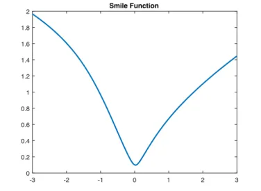
We will design the neural network according to the prior information. First, we introduce a new activation function, which we will name it smile func-tion.

Definition 1.4.1. Smile Function The smile function (z) is defines as

(z) = r (ztanh(z+ 1 2) + tanh( 1 2z+✏)) (1.10)

(24)

Here ✏ is a small value to ensure numerical stability, where we set

✏ = 0.01. The design of a smile function is inspired by the skew or smile pattern observed from implied volatility slice. It has some good properties: (i) it is a smooth function that can be di↵erentiated at least twice while maintaining the numeric stability (ii) it always produces positive values (iii) its shape is what the volatility curve is supposed to be: smile or skew pattern. It is illustrated by Fig. 1.1

-3 -2 -1 0 1 2 3 0 0.2 0.4 0.6 0.8 1 1.2 1.4 1.6 1.8 2 Smile Function

Figure 1.1: Smile Function

The input of neural network model consists of two variables: m and

⌧. Its output is the estimation of implied volatility: ˆv. Its objective is to minimise the di↵erence between the prediction ˆv and its ground-truth value v. We will first propose a model, called single model, as a base for modelling the IVS. After that, we will introduce the multi-model which is a data-driven combination of single models. One intuition for multi-model is each single model might capture only part of the IVS and a combination of these single models may lead to well behaved IVS model. In 1.4.2, we will provide an explanation on how the prior information is encoded into the single and multi model.

(25)

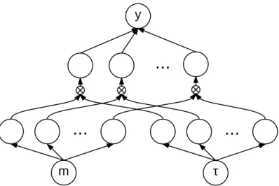
Figure 1.2: Single Model m

...

?

...

y

The proposed model (single). Note that bias terms exist, although they are omitted for neat appearance. _⌦is the multiplication gate that outputs the product of the inputs.

Single Model

The core of the single model can be written as,

ˆ v=y(m,⌧) = J X j=1 (mW¯1,j + ¯bj) (⌧W˜1,j+ ˜bj)e ˆ Wj,1_{+ e}ˆb _(1.11) Here (·) is the sigmoid function and (·) is the smile function. J is the number of neurons in the hidden layer. There are 6 parameters to learn: ¯b, ¯W, ˜b, ˜W, ˆW, and ˆb. Each of the first five parameters has J elements, and the last one ˆb has only one parameter, so the total number of parameters is 5J + 1.

We term Eq. 1.11 as our single model and an illustration can be seen in Fig. 2.1.

A very good property of the whole design of Eq. 1.11 is that, it will not generate negative values under any circumstances, and this is very important as the implied volatility is always positive. This is achieved by carefully choosing the activation functions, i.e., (·) and (·), as well as forcing the weight and bias terms of the top layer being positive by the exponential function, i.e., eWˆj,1 _{and e}ˆb_.

(26)

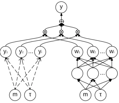
Figure 1.3: Multi Model

m

?

y

1

y

2

...

y

I

m

?

...

w

1

w

2

...

w

I

y

The proposed model (multi): The right side is the weight generating model, and the left side is a set of single models. Note that the left side is not a single layer. Each (m,⌧)!yi(linked by two dashed arrows) is realised by a full-sized single model. is

the addition gate that outputs the sum of the inputs.

Multi Model

Our final model, termed asmulti model, jointly trains multiple single mod-els, as well as a weighting model to softly switch them. As illustrated in Fig. 2.2, the full model’s left-hand side has i= 1. . . I single models:

yi(m,⌧) = J

X

j=1

(mW¯₁(_,ji)+ ¯b_j(i)) (⌧W˜₁(_,ji)+ ˜b(_ji)) ˆW_j,(i₁)+ ˆb(i) (1.12) Its right-hand branch is a network with oneK unit hidden layer, and the top layer has an I-way softmax activation function that provides a model selector for the left branch.

(27)

Description Shape # in Single Model # in Multi Model ¯

W weight term for moneyness 1⇥J 1 I

¯

b bias term for moneyness J 1 I

˜

W weight term for time-to-maturity 1⇥J 1 I

˜

b bias term for time-to-maturity J 1 I

ˆ

W weight term for final pricing J⇥1 1 I

ˆ

b bias term for final pricing 1 1 I

˙

W weight term for weighting model hidden 2⇥K 0 1

˙

b bias term for weighting model hidden K 0 1

¨

W weight term for weighting model output K⇥I 0 1

¨

b bias term for weighting model output I 0 1

Table 1.1: Parameters List

Finally, the overall output y is the softmax weighted average of the I local option pricing models’ outputs.

ˆ v = I X i=1 yi(m,⌧)wi(m,⌧) (1.14)

Due to the softmax activation, the sum of weights (wi’s) is one and the

weights are all positive. So the useful property of producing positive values only is preserved from single model to multi model.

The number of parameter in multi model is (5J+1)I+3K+(K+1)I = (5J +K+ 2)I+ 3K. The parameter list of single model and multi model is shown in Table 1.1.

Embedding Constraints

In this section, we will demonstrate how the prior information in Sec-tion 1.4.1 is encoded into our model design.

The first two conditions, positive and twice di↵erentiable, in no static arbitrage 1.4.1 are realised by the function form of our single model and multi model.

The conditions, monotonic and free of butterfly arbitrage in no static arbitrage 1.4.1 can be achieved by the technique generating pseudo training data and loss function explain in Section 1.2.2.

Monotonic Condition For monotonic condition,

(28)

We define a functionc(m,⌧) =v(m,⌧) + 2⌧ @⌧v(m,⌧) and our objective is to push c(m,⌧) to be non-negative.

To achieve this, we sampleP uniquemvalues: [m1, m2, . . . mP], andQ

unique ⌧ values: [⌧1,⌧2, . . .⌧Q], and add the following loss function,

`1= P X p=1 Q X q=1 max(0, c(mp,⌧q))

This is exactly what we discussed in Section 1.2.2: we generate a collec-tion of pseudo training data, i.e., P_⇥Qpairs of (m,⌧), and feed them into training process. The above loss function will generate a penalty if some negative values are produced by c(m,⌧) for a certain set of (m,⌧) pairs. Theoretically, if an infinite number of samples were generated and the loss function were to be reduced to zero during optimisation, the condition would be met while in practice it is not usually necessary to do so because for most real-world problems, the value of the input variable is usually at a reasonable interval, e.g.,m₂[ 3,3]. It is also unnecessary to extremely densely sample the pseudo-data; after all, the function of proposed neural networks is very smooth (infinitely di↵erentiable), so we do not need to worry should it behave impulsively.

Free of Butterfly Arbitrage For free of butterfly arbitrage condition,

g(m,⌧) = (1 m@mv(m,⌧) v(m,⌧) )

2 (v(m,⌧)⌧ @mv(m,⌧))2

4 +⌧v(m,⌧)@mmv(m,⌧)>0 Our objective is to push g(m,⌧) to be non-negative.

`2 = P X p=1 Q X q=1 max(0, g(mp,⌧q))

Boundary Condition For boundary condition,

(29)

• Left Boundary Condition

N( d (m,⌧)) +p⌧ @mv(m,⌧)n(d (m,⌧))>0 when m <0

We define two functionsb1(m,⌧) = N(d (m,⌧)) p⌧ @mv(m,⌧)n(d (m,⌧))

and b2(m,⌧) = N( d (m,⌧)) +p⌧ @mv(m,⌧)n(d (m,⌧)) and our

objec-tive is to push both of them to be non-negaobjec-tive.

To achieve this, we sampleP1unique non-negativemvalues: [m1, m2, . . . mP1], P2 unique negative m values: [m1, m2, . . . mP2], and Q unique ⌧ values: [⌧1,⌧2, . . .⌧Q], and add the following loss function,

`3= P1 X p1=1 Q X q=1 max(0, b1(mp1,⌧q)) + P2 X p2=1 Q X q=1 max(0, b2(mp2,⌧q))

Asymptotic Condition For asymptotic condition,

2|m| v2(m,⌧)⌧ >0

We define a function a(m,⌧) = 2|m| v2_(m,_⌧₎_⌧ _> _{and our objective}

is to push a(m,⌧) to be positive.

`4 = P X p=1 Q X q=1 max(0, (c(mp,⌧q) ✏))

Here✏= 10 5 _{is a small value.}

Regularisation To prevent over-fitting, we add `2 regularisation (a.k.a,

Frobenius norm) for all weight terms.

For a matrix of shapeI _⇥J,`2 regularisation is defined as,

||W_||2_F = 1 2 I X i=1 J X j=1 W_i,j2

(30)

thus reduce the complexity of the model.

In the single model, this will introduce a loss function,

`5 =||W¯||2F +||W˜ ||2F +||Wˆ ||2F

Similarly, for the multi model, the loss function is,

`5= I X i=1 ||W¯ (i)_||2F + I X i=1 ||W˜(i)_||2F + I X i=1 ||Wˆ(i)_||2F +||W˙ ||2F +||W¨||2F

Limit Condition The limit condition 1.4.1 is partly considered when we design the smile function as the exponent ofmin smile function is roughly 0.5. We expect that v(m,⌧) will grow slower thanm, hence the limit will approaching to ₁. We will only exam this numerically when we get the final model.

Loss Function Our main objective is to fit the ground-truth implied volatility, for which we combine two kinds of loss functions.

Mean Squared Log Error (MSLE) `MSLE_(y,_{y) =}_ˆ 1

N

PN

n=1(log(yn)

log(ˆyn))2

Mean Squared Percentage Error (MSPE) `MSPE_(y,_{y) =}_ˆ 1

N PN n=1( yn yˆn yn ) 2

The first component of our loss function is defined as,

`0 =↵`MSLE+ `MSPE

Apart from the fitting loss, we have four condition-related losses, `1,

`2,`3, and `4. They are corresponding to Monotonic Condition, Boundary

Condition, Free of Butterfly Arbitrage, Asymptotic Condition. Finally, we have`5, the loss with respect to regularisation.

In summary, the loss function is,

(31)

Prior Neural Network Model

Prior Neural Network Model For Single Model From the above

discussion, our prior neural network for single model is listed as following.

ˆ v(m,⌧) =y(m,⌧) = J X j=1 (mW¯1,j + ¯bj) (⌧W˜1,j + ˜bj)e ˆ Wj,1 _{+ e}ˆb _(1.15) with the loss function

`=`0+ `1+ `2+⌘`3+⇢`4+!`5 and • `0=↵`MSLE+ `MSPE – `MSLE_(v,_{v) =}_ˆ 1 N PN n=1(log(vn) log(ˆvn))2 – `MSPE_(v,_ˆ_{v) =} 1 N PN n=1(vnvnˆvn) 2 • `1= PP p=1 PQ q=1max(0, c(mp,⌧q)) • `2=PP_p₌₁PQ_q₌₁max(0, g(mp,⌧q)) • `3=PPp11=1 PQ q=1max(0, b1(mp1,⌧q))+ PP2 p2=1 PQ q=1max(0, b2(mp2,⌧q)) • `4=PP_p₌₁P_qQ₌₁max(0, (c(mp,⌧q) ✏)) • `5=||W¯||2F +||W˜||2F +||Wˆ||2F

where`0is the fitting loss and`1,`2,`3and`4, corresponding to Monotonic

Condition, Boundary Condition, Free of Butterfly Arbitrage, Asymptotic Condition are losses coming from prior information and`5isL2

regularisa-tion loss to prevent over-fitting We will use this prior deep neural network together with training data and pseudo-data to get the posterior deep neu-ral network for single model.

Prior Neural Network Model For Multi Model Our main model,

prior neural network model for multi model, is listed as following

ˆ v = I X i=1 yi(m,⌧)wi(m,⌧) (1.16)

(32)

where yi(m,⌧) is single model yi(m,⌧) = J X j=1 (mW¯1(,ji)+ ¯b (i) j ) (⌧W˜ (i) 1,j + ˜b (i) j ) ˆW (i) j,1 + ˆb(i) (1.17)

and wi(m,⌧) is the weighting model

wi(m,⌧) = ePKk=1 (mW˙1,k+⌧W˙2,k+˙bk) ¨Wk,i+¨bi PI i=1e PK k=1 (mW˙1,k+⌧W˙2,k+˙bk) ¨Wk,i+¨bi (1.18) with the loss function

`=`0+ `1+ `2+⌘`3+⇢`4+!`5 and • `0=↵`MSLE+ `MSPE – `MSLE_(v,_{v) =}_ˆ 1 N PN n=1(log(vn) log(ˆvn))2 – `MSPE_(v,_ˆ_{v) =} 1 N PN n=1( vn ˆvn vn ) 2 • `1=PPp=1 PQ q=1max(0, c(mp,⌧q)) • `2=PP_p₌₁PQ_q₌₁max(0, g(mp,⌧q)) • `3=PP_p₁1₌₁PQ_q₌₁max(0, b1(mp1,⌧q))+ PP2 p2=1 PQ q=1max(0, b2(mp2,⌧q)) • `4=PP_p₌₁P_qQ₌₁max(0, (c(mp,⌧q) ✏)) • `5=PI_i₌₁||W¯(i)||2F+ PI i=1||W˜ (i)||2F+ PI i=1||Wˆ(i)||2F+||W˙ ||2F+||W¨||2F

where`0is the fitting loss and`1,`2,`3and`4, corresponding to Monotonic

Condition, Boundary Condition, Free of Butterfly Arbitrage, Asymptotic Condition are losses coming from prior information and `5 is L2

regular-isation loss to prevent over-fitting We will use this prior neural network together with corresponding training data and psudo-data to get the pos-terior neural network in section 1.5.

(33)

1.5

Empirical Results

1.5.1

Data sets

The options data for S&P500 index comes from OptionMetrics, which pro-vides historical End-Of-Day bid and asks for quotes. The data sample covers the period from 04/01/1996 to 29/04/2016, which has 5116 trad-ing days. OptionMetrics also provides zero coupon yield curve which is constructed using LIBOR rates. However, we know that after the 2008 financial crisis, the traditional LIBOR-based zero curve is certainly not risk-free. Hence, I download the overnight index swap (OIS) rates from Bloomberg and bootstrap the zero rate curve from these rates starting from 01/01/2008 to 29/04/2016. Before 01/01/2008, I still use the zero rate curve provided by OptionMetrics. The risk-free rates are interpolated using cubic spline to match the option maturity. Forward price is inferred from put-call parity. I find this is better than using the constant dividend rate provided by OptionMetrics to calculate the forward price.

Several data filters should be carried out before model calibration. I exclude all option quotes less than 3/8 as these prices may be misleading due to close to tick size. Bid-ask mid-point price is calculated as a proxy for closing price. I discard in-the-money put and call option quotes as out-of-the-money options are more reliable than less traded in-out-of-the-money options. Unlike the majority of the paper in the implied information construction literature [Jiang and Tian, 2005, Bakshi et al., 2003, Bondarenko, 2014], which only keeps few contracts on each day and ignore all option contracts with time to maturity less than 7 days, I only omit the contract which has a maturity date of less than 2 days and keep as many contracts as possible. Options with a short maturity, like weekly index options, are getting more and more popular over recent days. Hence, it is necessary to keep them rather than just discard them. This will clearly increase the difficulty in programming and requires stability in optimization. Fortunately, this is not a daunting job for neural network. After these operations, there are 63338 option contracts with 2,986,754 valid quotes. All these valid quotes are converted into implied volatility through BS formula.

(34)

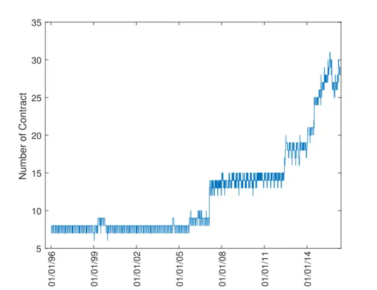
contracts and the number of valid quotes after filter on each day in the following Figures 1.4 and 1.5. The number of contracts rarely exceed 10 before 2007. It almost doubled from 2007 to 2012. Recently, it reached more than 30 contracts on each day. This is a good news for implied volatility surface as this increase the number of di↵erent time to maturity. Due to the increase of number of contracts, the number of valid quotes share a similar profile. The number of valid quotes is under 300 before 2007. It increases to around 1000 before 2013. Recently, it even reaches more than 3000 quotes per day. This is sufficient for fitting implied volatility surface. Furthermore, we also plot the log forward moneyness of S&P500 index options in the Figure 1.7 and the range of time to maturity in the Figure 1.6. It is clear that majority of the log forward moneyness lies in the range of -2.5 to 0.5. This causes problems for neural network as it can’t learn anything beyond this range. If we blindly use arbitrary neural network, the final model will be unpredictable as the shape of the IVS beyond the range of -2.5 to 0.5 can be anything. This is the reason that we introduce prior information to pose some constraints on the shape of IVS.

1.5.2

Implementation details

We implement the neural network models using TensorFlow2_{. Neural}

net-work modes are usually trained by gradient-based method, but it is a bit tricky to choose the optimal step-size (a.k.a. learning rate) for gradient descent. A common choice is to slowly reduce the step-size after every iter-ation, however, how to determine the initial learning rate is still a problem. Modern optimisation methods for neural network often employ a kind of automatic adjustment according to the scale of gradient, so they are less sensitive to the choice of initial learning rate. Here we choose to use Adam [Kingma and Ba, 2015] for optimisation because of its popularity in deep learning.

(35)

Figure 1.4: The Change of Number of Contracts 01/01/96 01/01/99 01/01/02 01/01/05 01/01/08 01/01/11 01/01/14 5 10 15 20 25 30 35 Number of Contract

This is the number of contracts available every day after data filter. The data sample covers the period from 04/01/1996 to 29/04/2016, which has 5116 trading days. The number of contracts rarely exceed 10 before 2007. It almost doubled from 2007 to 2012. Recently, it reached more than 30 contracts on each day. This is a good news for implied volatility surface as this increase number of di↵erent time to maturity.

1.5.3

Baseline Models

Our main model is multi model, and for benchmark, we compare it with the following baseline methods: single model, SSVI. Besides, We implement a vanilla feed-forward neural network model (named vanilla model) that uses the same input, but has no specific designs for the nature of problem. Vanilla model has one hidden layer with sigmoid activation function and a constraint that ensures positive output. Furthermore, for all those neural network models, we use two di↵erent settings (i) full model (ii) model with fitting purpose only, i.e., we disable all loss functions related to conditions, thus the existing loss functions are `0 and`5. The specified model without

(36)

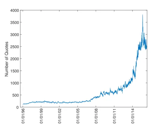
Figure 1.5: The Change of Number of Quotes 01/01/96 01/01/99 01/01/02 01/01/05 01/01/08 01/01/11 01/01/14 0 500 1000 1500 2000 2500 3000 3500 4000 Number of Quotes

This is the number of valid quotes available every day after data filter. The data sample covers the period from 04/01/1996 to 29/04/2016, which has 5116 trading days. The number of valid quotes is under 300 before 2007. It increases to around 1000 before 2013. Recently, it even reaches more than 3000 quotes on each day. This is sufficient for fitting implied volatility surface.

is written as multi* model.

Hyper-parameters

multi model removes all loss functions w.r.t prior information. (only fitting loss `0 and regularisation loss `5.) We list all hyper-parameters for neural

network models in Table 1.2. Note that one key consideration is to control the model size in terms of the number of parameters to learn, so that di↵erent models have very close number of parameters. This is to reduce the chance that di↵erence in model performance is caused by model size.

(37)

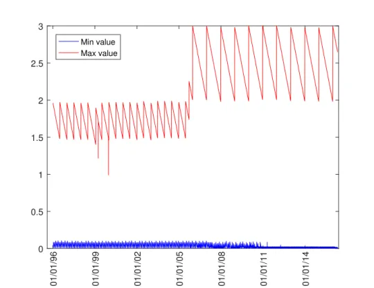
Figure 1.6: Range of Time to Maturity 01/01/96 01/01/99 01/01/02 01/01/05 01/01/08 01/01/11 01/01/14 0 0.5 1 1.5 2 2.5 3 Min value Max value

This is the minimum and maximum of time to maturity of all contracts available every day after data filter. The data sample covers the period from 04/01/1996 to 29/04/2016, which has 5116 trading days. The range of time to maturity is between 0 and 3.

Sample Mechanism

To meet those conditions, we need to generate pseudo-data. We carefully control the ratio of real market data and pseudo-data, and the empirical choice is 1 : 6. For asymptotic condition, we sample log-moneyness in [ 6, 3][[3,6]. For other conditions, the range of log-moneyness sam-pled is [ 3,3]. The range of time-to-maturity sampled is [0.002,3]. The choice on these ranges is based on the observations from historical data, see Fig. 1.7 and Fig. 1.6.

1.5.4

Numerical Experiment

To test the performance of our multi model, we compare both in-sample performance and out-of-sample performance with other baseline models

(38)

Figure 1.7: Range of Log-Moneyness 01/01/96 01/01/99 01/01/02 01/01/05 01/01/08 01/01/11 01/01/14 -3.5 -3 -2.5 -2 -1.5 -1 -0.5 0 0.5 1 Min value Max value

This is the minimum and maximum of log forward moneymess of all contracts available every day after data filter. The data sample covers the period from 04/01/1996 to 29/04/2016, which has 5116 trading days. It is clear that the majority of the log forward moneyness lies in the range of -2.5 to 0.5. This causes problems for neural network as it can’t learn anything beyond this range. If we blindly use arbitrary neural network, the final model will be unpredictable as the shape of the IVS beyond the range of -2.5 to 0.5 can be anything. This is the reason that we introduce prior information to pose some constraints on the shape of IVS.

mentioned in subsection 1.5.3. The performance criterion is mean average percentage error (MAPE) of implied volatility and MAPE of corresponding option prices.

There are 5116 trading days. On each trading day, we fit all the models using filtered option quotes available on that day to compute the MAPE of implied volatility and transform implied volatilities back to prices to calcu-late the MAPE of option prices. We call them Train IV (implied volatility) MAPE and Train Price MAPE. Furthermore, as our purpose is to build a

(39)

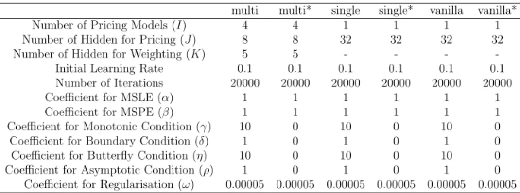
Table 1.2: Hyper-parameter for neural network models

multi multi* single single* vanilla vanilla*

Number of Pricing Models (I) 4 4 1 1 1 1

Number of Hidden for Pricing (J) 8 8 32 32 32 32

Number of Hidden for Weighting (K) 5 5 - - -

-Initial Learning Rate 0.1 0.1 0.1 0.1 0.1 0.1

Number of Iterations 20000 20000 20000 20000 20000 20000

Coefficient for MSLE (↵) 1 1 1 1 1 1

Coefficient for MSPE ( ) 1 1 1 1 1 1

Coefficient for Monotonic Condition ( ) 10 0 10 0 10 0

Coefficient for Boundary Condition ( ) 1 0 1 0 1 0

Coefficient for Butterfly Condition (⌘) 10 0 10 0 10 0

Coefficient for Asymptotic Condition (⇢) 1 0 1 0 1 0

Coefficient for Regularisation (!) 0.00005 0.00005 0.00005 0.00005 0.00005 0.00005

Hyper-parameter for neural network models. model with * means the specified model without constraints

monotonic condition, left boundary condition, right boundary condition, butterfly arbitrage condition and asymptotic condition. We calculate the median of these violation percentage in each quarter for all models and plot them in Figure 1.9. Obviously, the model with constraints has much fewer violations than the corresponding one without constraints. Mean-while, multi model has the least violation with a scale of round 10 4_{, much}

smaller than single model and vanilla model. This means the prior informa-tion introduced in our framework does help to alleviate arbitrage situainforma-tions considerably. Furthermore, a blind usage of neural network, like vanilla* model (vanilla model without conditions), will lead to large percentage of arbitrage violations.

To verify the out-of-sample performance, we employ the above trained models to predict the implied volatilities for the next trading day to com-pute MAPE of implied volatility and MAPE of option price. These two MAPEs are named as Test IV MAPE and Test Price MAPE.

We calculate the mean and standard deviation in Table 1.3 and 1.4 for these MAPEs. Clearly, multi model is the best for both in-sample and out-of-sample performance. The superiority of multi model over single model indicates our intuition that each single model might capture only part of the IVS and combination of these single models may lead to well behaved IVS model is sensible. Furthermore, the superiority of multi model and single model over the vanilla model shows our design approach is much better

(40)

than blind usage of neural network. Last but not least, the superiority of multi model over SSVI illustrates a well-designed data-driven method has the potential to surpass some existing models in mathematical finance literature.

In Figure 1.8, we calculate mean of in-sample and out-of-sample MAPEs in each quarter for multi model, single model, vanilla model and SSVI and plot them to show the performance of each method. These graph shows again that multi model is the best for both in-sample and out-of-sample performance.

There are two conditions we have yet to discuss and indicate their neces-sity, namely, to limit condition and regularisation condition. We illustrate them by investigating their performance on a single day.

In Figure 1.10, we plot the implied volatility surface of multi model (above) and multi model without regularisation (below) on 2016/01/11. The graph for multi model without regularisation seems a bit over-fitting while the multi model above looks normal. The necessity of regularisation is even obvious if we look into the risk neutral density of forward return extracted from the corresponding IVS. In Figure 1.11, we plot the risk neu-tral density extracted from multi model (above) and multi model without regularisation (below) for forward return with duration 11, 32, 109 and 704 days. The risk neutral density for 109 and 704 days in multi model without regularisation appears quite strange compared with those in multi model.

For limit condition, we plot thed+(m,⌧) as a function of m for multi

model on 2016/01/11 with ⌧ equal to 11, 32, 109 and 704 days. The tendency of going to ₁ verifies the limit condition.

1.6

Conclusion

Our contribution lies in the following parts

• Our data sample is much larger than the majority of the work in modelling the IVS. We employ the HPC provided by Imperial College London to make this research possible.

(41)

Table 1.3: Train and Test IV MAPE

Model Train Mean. Train Std. Test Mean. Test Std.

multi model 1.74 0.50 3.34 2.18 multi* model 1.76 0.50 3.35 2.17 single model 2.15 0.67 3.60 2.12 single* model 1.82 0.52 3.38 2.16 ssvi 2.59 0.85 3.73 2.18 vanilla model 3.21 0.98 4.46 2.07 vanilla* model 2.87 0.80 4.18 2.04

This table computes the mean and standard deviation of Train and Test IV (implied volatility) MAPE in percentage. There are 5116 trading days. On each trading day, we fit all the models using filtered option quotes available on that day to compute the MAPE of implied volatility. The mean and standard deviation for the Train IV MAPE are listed in the first and second column. To verify the out-of-sample performance, we employ the above trained models to predict the implied volatilities for the next trading day to compute MAPE of implied volatility. The mean and standard deviation for the Test IV MAPE are listed in the third and fourth column.Clearly, multi model is the best for both in-sample and out-of-sample performance.Model with * means the specified model without constraints.

Table 1.4: Train and Test Price MAPE

Model Train Mean. Train Std. Test Mean. Test Std.

multi model 5.97 1.86 10.64 6.72 multi* model 6.03 1.86 10.67 6.70 single model 7.38 2.57 11.64 6.68 single* model 6.20 1.91 10.77 6.67 ssvi 8.71 2.72 12.74 6.74 vanilla model 11.31 3.57 14.61 6.42 vanilla* model 10.53 3.34 14.17 6.60

This table computes the mean and standard deviation of Train and Test Pricing MAPE in percentage. There are 5116 trading days. On each trading day, we fit all the models using filtered option quotes available on that day to calculate the MAPE of option prices. The mean and standard deviation for the Train Pricing MAPE are listed in the first and second column. To verify the out-of-sample performance, we employ the above trained models to predict the implied volatilities for the next trading day to compute MAPE of option prices. The mean and standard deviation for the Test Pricing MAPE are listed in the third and fourth column.Clearly, multi model is the best for both in-sample and out-of-in-sample performance.Model with * means the specified model without constraints.

(42)

Figure 1.8: Train and Test IV&Price MAPE

(a) Train IV MAPE

01/96 01/99 01/02 01/05 01/08 01/11 01/14 0.01 0.015 0.02 0.025 0.03 0.035 0.04 0.045 0.05 0.055 0.06 multi model single model vanilla model ssvi

(b) Train Price MAPE

01/96 01/99 01/02 01/05 01/08 01/11 01/14 0.04 0.06 0.08 0.1 0.12 0.14 0.16 0.18 0.2 0.22 multi model single model vanilla model ssvi (c) Test IV MAPE 01/96 01/99 01/02 01/05 01/08 01/11 01/14 0.01 0.02 0.03 0.04 0.05 0.06 0.07 multi model single model vanilla model ssvi

(d) Test Price MAPE

01/96 01/99 01/02 01/05 01/08 01/11 01/14 0.06 0.08 0.1 0.12 0.14 0.16 0.18 0.2 0.22 0.24 multi model single model vanilla model ssvi

We calculate the mean of in-sample and out-of-sample MAPEs in each quarter for multi model, single model, vanilla model and SSVI and plot them to show the performance of each method. These graph shows again that multi model is the best for both in-sample and out-of-sample performance.

(43)

Figure 1.9: Percentage of Violation (a) multi 01/01/96 01/01/99 01/01/02 01/01/05 01/01/08 01/01/11 01/01/14 01/01/17 0 0.5 1 1.5 2 2.5×10-4 Monotonic Condition Left Boundary Condition Right Boundary Condition Free of Butterfly Arbitrage Asymptotic Condition (b) single 01/01/96 01/01/99 01/01/02 01/01/05 01/01/08 01/01/11 01/01/14 01/01/17 0 0.002 0.004 0.006 0.008 0.01 0.012 0.014 Monotonic Condition Left Boundary Condition Right Boundary Condition Free of Butterfly Arbitrage Asymptotic Condition (c) vanilla 01/01/96 01/01/99 01/01/02 01/01/05 01/01/08 01/01/11 01/01/14 01/01/17 0 0.5 1 1.5 2 2.5 3 3.5×10-3 Monotonic Condition Left Boundary Condition Right Boundary Condition Free of Butterfly Arbitrage Asymptotic Condition (d) multi* 01/01/96 01/01/99 01/01/02 01/01/05 01/01/08 01/01/11 01/01/14 01/01/17 0 0.05 0.1 0.15 0.2 0.25 Monotonic Condition Left Boundary Condition Right Boundary Condition Free of Butterfly Arbitrage Asymptotic Condition (e) single* 01/01/96 01/01/99 01/01/02 01/01/05 01/01/08 01/01/11 01/01/14 01/01/17 0 0.05 0.1 0.15 0.2 0.25 Monotonic Condition Left Boundary Condition Right Boundary Condition Free of Butterfly Arbitrage Asymptotic Condition (f) vanilla* 01/01/96 01/01/99 01/01/02 01/01/05 01/01/08 01/01/11 01/01/14 01/01/17 0 0.05 0.1 0.15 0.2 0.25 Monotonic Condition Left Boundary Condition Right Boundary Condition Free of Butterfly Arbitrage Asymptotic Condition

On each trading day, we fit all the models using filtered option quotes available on that day and compute the percentage of violation in pseudo data for monotonic condition, left boundary condition, right boundary condition, free of butterfly arbitrage condition and asymptotic condition. We calculate the median of these percentage of violation in each quarter for all models and plot them. Obviously, the model with prior information has much less violations than the corresponding one without prior information. Meanwhile, the multi model has the least violation with a scale of round 10 4, much smaller than the single model and vanilla model. This means the prior information introduced in our framework does help to alleviate arbitrage situations considerably. Furthermore, a blind usage of neural network, like vanilla* model (vanilla model without conditions), will lead to a large percentage of arbitrage violations. Model with * means the specified model without constraints.

(44)

Figure 1.10: Comparison of Implied Volatility Surface 6 0 4 -6 0.5 time-to-maturity -4 1 implied volatility log-moneyness -2 2 1.5 0 2 2 2.5 0 4 6 0 4 -6 time-to-maturity 1 -4 2 log-moneyness -2 implied volatility 2 0 3 2 4 0 4

We plot the implied volatility surface of multi model (above) and multi model without regularisation (below) on 2016/01/11. The graph for multi model without regularisation seems a bit over-fitting while the multi model above looks normal.

(45)

Figure 1.11: Comparison of Risk Neutral Density -1 -0.8 -0.6 -0.4 -0.2 0 0.2 0.4 0.6 0.8 1 return 0 2 4 6 8 10 12 probability 11 Days 32 Days 109 Days 704 Days -1 -0.8 -0.6 -0.4 -0.2 0 0.2 0.4 0.6 0.8 1 return 0 2 4 6 8 10 12 probability 11 Days 32 Days 109 Days 704 Days

We plot the risk neutral density extracted from multi model (above) and multi model without regularisation (below) for forward return with duration 11, 32, 109 and 704 days. The risk neutral density for 109 and 704 days in multi model without regularisation looks quite strange compared with those in multi model.

(46)

Figure 1.12: Limit Condition Check 0 100 200 300 400 500 600 log-moneyness -600 -500 -400 -300 -200 -100 0 d + (m, τ ) 11 Days 32 Days 109 Days 704 Days

we plot thed+(m,⌧) as a function ofmfor multi model on 2016/01/11 with⌧ equal to

(47)

Approach, on how to design a deep neural network combined with economic assumptions. This guideline can be used for any modelling purpose rather than just modelling the IVS.

• Our multi model has better performance, in-sample and out-of-sample, than benchmark model SSVI. This illustrates a well-designed data-driven method has the potential to surpass some existing models in mathematical finance literature.

• There is still plenty of room to boost the multi model by investigating the model hyper-parameters.

• The multi model has the potential to be used in the HF option data.

• There is not many research working on how to combine machine learning, mathematical finance and finance in a coherent way to solve some modelling problems.

(48)

Chapter 2

Neural Network for Call

Option Pricing: Bayesian alike

Design Approach

2.1

Introduction

Yang et al. [2017] who propose a gated neural network for pricing European call options. They integrate assumptions of a valid call option surface from classical mathematical finance literature into neural network as inductive bias. Yang et al. [2017] can be reformulated in the form of Bayesian alike design approach in Chapter 1.

Option pricing models have long been a popular research area. From a theoretical perspective, new option pricing models provide an opportunity for academics to examine financial markets’ mechanics. From a practical viewpoint, market makers desire efficient pricing models to set bid and ask prices in derivative markets. The earliest and simplest pricing model, Black–Scholes Black and Scholes [1973a] gives a rough theoretical estimate of European option price. Since then many studies have attempted to find better option pricing models by relaxing the strict assumptions in Black– Scholes. The models proposed by mathematical finance literature usually start from a set of economic assumptions and end up with a deterministic formula that takes as input some market signals (e.g., moneyness, time

(49)

solve option pricing in a data-driven way: as a regression problem, with similar inputs to mathematical finance models, and real market option prices as outputs. The complicated relationship between input and output (e.g., a Black–Scholes like formula) is learned from a large amount of data rather than derived from economic axioms. Progress in data-driven option pricing can be driven by improvements in model expressibility, as well as integrating selected economic axioms into a data-driven model as prior knowledge. In this paper we employ the Bayesian alike design approach to rederive the results of call option pricing from Yang et al. [2017].

Regression models trained by machine learning techniques, such as ker-nel machines and neural networks, generalise well to out-of-sample cases as long as the training data is sufficient. Such data-driven methods give good option price estimates Malliaris and Salchenberger [1993], and can even surpass formula derived from economic principles. One drawback of existing data-driven approaches is that they seek a unique solution for all options. However, learned pricing models fail on certain options, for example, some overestimate deep out-of-the money options Bennell and Sutcli↵e [2004], or underestimate options very close to maturity Dugas et al. [2000]. To alleviate these issues, Gradojevic et al. [2009] proposed a ‘divide-and-conquer’ strategy, by first grouping options into sub-categories, and building distinct pricing models for each sub-category. However, this categorisation is done by manually defined heuristics, and may not be con-sistent with market conditions, and their changes in time. In this paper, we propose a novel class of neural networks for option pricing. These im-plement a divide-and-conquer