Implications of the design of monetary policy for financial stability

(1)

IMPLICATIONS OF THE DESIGN OF MONETARY POLICY FOR FINANCIAL STABILITY

Alicia García Herrero and Pedro del Río1

Abstract

This paper is a contribution to the literature on the factors behind financial stability, focusing on monetary policy design. In particular, it assesses empirically for a sample of 79 countries in the period 1970 to 2000 whether the choice of the central bank objectives and the monetary policy strategy affect financial stability. We find that focusing the central bank objectives on price stability reduces the likelihood of a banking crisis. This result is robust to several model specifications and groups of countries. As regards the monetary policy strategy, exchange rate targeting significantly reduces the likelihood of a banking crisis for some model specifications and, in particular, for the group of countries in transition.

JEL Classification: E52, E44, G21

Key words: Monetary policy design, monetary policy objectives, monetary policy strategy, financial stability, and banking crisis

1

Both authors are affiliated with Banco de España. The opinions expressed are those of the authors and not of the institution they represent. Corresponding author: [email protected] (+0034913387032)

(2)

1. INTRODUCTION

The relation between monetary policy and financial stability has been long debated but there is still no clear consensus on how one affects the other and, in particular, whether the are trade-offs or synergies between them. This is clearly an important issue, which deserves further attention, since it could help devise arrangements and policy responses to promote both monetary and financial stability.

We look into the role that the design of monetary policy may have in fostering financial stability, in particular the choice of the central bank objectives and the monetary policy strategy. More specifically, we assess empirically whether countries whose central banks focus narrowly on price stability are less prone to financial instability, when accounting for other factors. In the same vein, we test which monetary policy strategy (exchange rate based, money or inflation targeting), if any, best contributes to financial stability.

The motivation for focusing on monetary policy as a potential factor contributing to financial stability stems from the encouragingly growing literature on the role of institutions and policy design. In the particular case of financial stability, the rationale is that an appropriate institutional and policy design should foster a better credit culture and an effective market functioning. The design of monetary policy should be particularly important since the central bank is probably the most relevant institution for the performance of the banking system.

2. EXISTING LITERATURE

What do we mean by financial instability?

Financial stability is an elusive concept to define. The literature has mainly focused on

its extreme realization, the occurrence of a financial crisis, mainly a banking crisis.

According to Mishkin (1996) a financial crisis is a disruption to financial markets in which adverse selection and moral hazard become much worse, so that financial markets are unable to efficiently channel funds to those who have the most productive investment opportunity. A very different definition of a financial crisis is given by Bordo, Mizrach and Schwartz (1995) where a real - as opposed to pseudo - financial crisis is a flight to cash because of the perception that no institution will supply the necessary liquidity. These

(3)

different definitions reflect the opposing theories concerning the causes of financial crisis: asymmetric information in the former and monetary developments in the latter. In any case, both definitions include the danger of a failure of financial and/or non-financial firm.

Bernanke and Gertler (1990) offer a broader concept of financial instability based on the term financial fragility. This is the situation in which potential borrowers have low wealth relative to the size of their projects. Such a low insider’s stake increases the agency problem and exacerbates frictions in the credit market (balance sheet channel). Finally,

financial instability is sometimes used synonymously to asset price volatility which takes

prices far away from their fundamental level, finally reversing suddenly and producing a

“crash” (Bernanke and Gertler (2000), Crockett (2000)).

In this work, we are interested in the first type of definition of financial instability (financial crisis), with special focus on the banking system, being what central banks can influence the most. The IMF (1998) has coined a definition that focuses on this; namely, banking crises are situations in which actual or potential bank runs or failures induce banks to suspend the internal convertibility of their liabilities or which compel the government to extend assistance to banks on a large scale. Another more general definition by Gupta (1996) is a situation in which a significant group of financial institutions have liabilities exceeding the market value of their assets, leading to portfolio shifts or to deposit runs and/or the collapse of financial institutions and/or government intervention. Under such circumstances, an increase in the share of non-performing loans, an increase in financial losses, and a decrease in the value of the bank’s investments cause solvency problems and may lead to liquidations, mergers and restructuring of the banking system. Both definitions, and others which focus on the banking system, boil down to the description of a banking crisis. However, the complexity of these definitions indicates that no single quantitative indicator can proxy a banking crisis accurately enough. An additional problem is the lack of comparable cross-country data to construct such indicator (i.e., the share of non-performing loans or risk-weighted capital to asset ratios). This is why the empirical literature has opted for

identifying banking crisis as events, expressed through a binary variable, constructed

with the help of cross-country surveys (Lindgreen et al. (1996), Caprio and Klingebiel

(4)

Determinants of financial stability

The economic literature has mostly concentrated on the macroeconomic determinants of financial stability and, to a lesser extent, on the financial sector determinants. Among the former, the main ones are: low growth or recessions (Frankel and Rose (1998)); too high real interest rates (Demirgüc-Kunt and Detragiache (1998)), large capital inflows

(Calvo (1997)), and shocks to inflation or the price level (Bordo et al. (2000), English

(1999), Hardy and Pazarbasioglu (1999)). The last one is in part related to the way monetary policy is conducted, in so far as monetary policy aims at price stability, and

thus it is related to our research objective. Among the latter, excessive credit growth2

(Gavin and Hausmann (1996), Sachs et al. (1996)), low levels of liquidity in the banking

system (Calvo (1997)), and bank currency mismatches (Chang, Céspedes and Velasco (2000)).

Less attention has been paid to the impact of institutional and policy design, with some exceptions; in particular the role of the legal framework (La Porta et al. (1998)) and that of the deposit insurance scheme (Demirguc-Kunt and Detragiache (2000)). The focus of our paper will be policy design, and in particular the monetary policy framework. The existing literature on monetary policy design has concentrated on issues different than financial stability (mainly price stability but also output stabilization). There is some more empirical analysis, albeit still scarce, on the reverse issue, namely the impact of financial instability, and in particular banking crises, on a country’s monetary policy. García Herrero (1997) and Martinez Peria (2000) find empirical evidence that money demand is stable in the long run in countries having experienced systemic banking crises. However, they do not test whether the design of monetary policy can reduce the likelihood of a banking crisis.

This issue is related to the very much debated question of the relation between price stability and financial stability. The economic literature is divided as to whether there are synergies or a trade-off between them. Among the arguments for a trade-off, Mishkin (1996) argues that high level of interest rates, necessary to control inflation, negatively affect banks’ balance sheets and firms’ net financial worth, especially if they attract capital inflows, contributing to over-borrowing and increasing credit risk, as well as currency mismatch if foreign capital flows into domestic-currency denominated loans. Cukierman (1992) states that inflation control may require fast and substantial increases

(5)

in interest rates, which banks cannot pass as quickly to their assets as to their liabilities, increasing the interest rate mismatch and, thus, market risk. Finally, Blinder (1999), Crockett (2000) and Viñals (2001) argue that a protracted period of price stability may lead to an inappropriate discounting of economic risks due to myopic growth expectations in countries which are no t used to price stability. Among the arguments for synergies between price and financial stability, Schwartz (1995) and Bordo (1985) state that credibly maintained prices provide the economy with an environment of predictable interest rates, contributing to a lower risk of interest rate mismatches, minimizing the inflation risk premium in long-term interest rates and, thus, contributing to financial soundness.

3. PURPOSE OF THE STUDY

This paper builds upon the exiting literature on how to foster financial stability, focusing on the role of monetary policy design. In particular, it assesses empirically whether the choice of the central bank objectives and the monetary policy strategy affect financial stability.

Monetary policy can have important implications for financial stability. On the one hand, if monetary policy is too lax, inflation will probably increase and become more volatile. Positive inflation surprises redistribute real wealth from lenders to borrowers contracting in nominal (non-indexed) loan instruments. Negative inflation surprises have the opposite effect. Redistribution in either direction may provoke bankruptcy, with serious implications for the quality and performance of banks' loans. On the other hand, a very tight monetary policy leading to very low inflation levels and, thereby, very low interest rates, may increase financial instability because it makes cash holdings more attractive in comparison with interest-bearing bank deposits. Any switch away from bank deposits is liable to reduce the profits earned by banks. In the same vein, if tight monetary policy does not manage to bring down inflation and real interest rates remain high, financial stability might be at risk. Sharp increases in real interest rates may have adverse effects on the balance sheets of banks and may produce a credit crunch. There is, thus, no

clear a priori sign whether too lax or too tight monetary policy is best for financial

stability.

2

It is interesting to note that lending booms are often deemed as the domestic counterpart of large capital inflows (Gourinchas et al. (2001)).

(6)

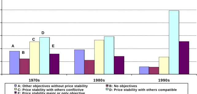
The objectives set for the central bank and the way to achieve them – the monetary policy strategy – are crucial policy elements determining whether monetary policy will be too lax or too tight. We shall, thus, focus on these two aspects in our empirical study. Since their creation, central banks have moved back and forth in the objectives they have targeted. In the last decade, the trend has been towards narrowing down the central bank objectives to a single one, price stability, or at least to a set of objectives considered to be compatible with price stability (see Figure 1). However, many other situations still exist: some central banks aim at price stability together with other - in principle non-compatible – objectives; others do not include price stability in their list of objectives or do not have such thing as declared objectives.

Figure 1: Distribution of Central Bank Objectives by Decades 0 10 20 30 40 50 60 1970s 1980s 1990s %

A: Other objectives without price stability B: No objectives

C: Price stability with others conflictive D: Price stability with others compatible E: Price stability major or only objective

A B

C D

E

The trend towards objectives with a greater focus on price stability, however, seems to be more related to the relatively larger importance given to price stability in the literature than to the conviction that it can contribute to financial stability. This is partly due to the lack of consensus whether synergies - or a trade-off - exist between price and financial stability. If synergies exist, a central bank focusing on price stability should be able to promote financial stability as well as price stability. However, if there is a trade-off, a central bank with multiple objectives should be able to take this trade-off better into account.

(7)

the advantages and disadvantages of each strategy for achieving price stability but hardly any evidence exists on how it affects other potential objectives, such as financial stability. While this might be the right way to choose the strategy – it avoids using one single instrument for too many objectives - it is still interesting to know whether there are spill-overs from the choice of the strategy towards financial stability.

When compared with the central bank objectives, the reasons why the choice of the monetary policy strategy can affect financial stability are less clear-cut. Perhaps the most debated case is the exchange-rate based strategy, at least as concerns the impact of a relatively fixed exchange rate regime on the probability of a banking crisis. But even in this case, where empirical evidence exists, there is no consensus (Domaç and

Martinez Peria, 2000). There is, thus, hardly any a priori on which strategy can better

contribute to financial stability.

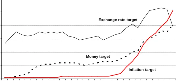
A historical overview of the monetary policy strategies (based on our data sample) adopted over time shows that the number of central banks with direct inflation targeting strategies has surged from close to zero at the end of the 1980s to over 50 today. The number of central banks targeting a monetary aggregate has also grown albeit less rapidly; they are nearly 40 today. On the contrary, central banks with an exchange rate anchor are less than 40 today from over 50 in the mid 1990s (see Figure 2). This corresponds with a certain degree of disenchantment with fixed exchange rates, after the Mexican and Asian crises. The information available also shows that more and more central banks have more than one monetary policy strategy, which could be understood as a growing preference for a certain degree of flexibility.

(8)

Figure 2: Evolution of Monetary Policy Strategies (number of countries) 0 10 20 30 40 50 60 1970 1971 1972 1973 1974 1975 1976 1977 1978 1979 1980 1981 1982 1983 1984 1985 1986 1987 1988 1989 1990 1991 1992 1993 1994 1995 1996 1997 1998 1999

Exchange rate target

Money target

Inflation target

4. VARIABLE DEFINITIONS AND DATA

We now describe the definitions chosen for our dependent variable, financial instability, and the objective variables (central bank objectives and the monetary policy strategy) as well as the source of the data. Finally, the control variables introduced are briefly described.

Among the different definitions given to financial stability, we concentrate on its extreme realization, namely a crisis event. We concentrate on banking crises, banks being the major player in most countries’ financial system and influenced most directly by the central bank. Future extension of the work aims at including broader definitions of bank unsoundness, which look not only into extreme cases (crises) but into bank fragility, based on indicators of bank solvency, profitability and efficiency.

To account for banking crisis, we use existing different surveys of crisis events and identify periods of systemic and non-systemic crises according to the information and chronology of episodes provided by Caprio and Klingebiel (2003) and Domaç and Martinez Peria (2000). We choose these surveys because they are the most comprehensive and updated. We check for potential inconsistencies between the two, which sometimes exist particularly for the dating of crisis, and support our choice with other sources (such as IMF staff reports, and financial news) in these specific cases. It should be noted that it is difficult to identify the timeframes of banking crises and to

(9)

differentiate between systemic and non-systemic cases, but according to the authors the dates attached to the crises are those generally accepted by finance experts. We also follow their definition of a systemic banking crisis as the situation when much or all of bank capital is exhausted. The list of crisis events determining our dependent variable, its classification into systemic and non-systemic episodes and their duration is provided in Table A2 of the Appendix. In addition, a detailed description of the sources and construction of all variables can be found in the Appendix.

We now move to the aspects of monetary policy design chosen as objective variables. The first summarizes the type of central bank objectives into an index which we

construct following the approach of Cukierman et al. (1992). This takes a larger value

the more narrowly the central bank statutory objectives focus on price stability. More specifically, it takes the value of 1 when price (or exchange rate) stability is the only or main goal. It takes the value of 0.75 when the objective of price stability is accompanied by - in principle non-conflicting - monetary objectives, such as financial stability. It takes the value of 0.50 when price stability goes together with others - in principle conflicting – objectives, such as economic growth and/or employment creation. This is the case when objectives such as employment or growth are stated separately without being qualified by statements such as “without prejudice to monetary or price stability”. Finally, the index takes the value of 0.25 when there are no statutory objectives and 0 when none of the existing goals is price stability. This index is constructed with the information provided by Cukierman, Webb and Neyapti (1992), Mahadeva and Sterne (2000) and Cukierman, Miller and Neyapti (2002) in the case of accession countries. The list of objectives and countries is available by decades, so we have assumed them to be constant through every year of each decade.

The second objective variable is the monetary policy strategy that a central bank follows. Strategies mainly differ in the choice of the intermediate variable which should help achieve the central bank objectives. Strategies are, thus, classified into exchange rate targeting, monetary and direct inflation targeting. Three dummy variables are created, one for each strategy, which take the value of one when the central bank uses that specific strategy and zero otherwise. It should be noted that these dummies are not mutually excludable. In other words, there may be countries whose central banks use two different monetary strategies in parallel. One example is that of Spain during the last years of participation in the ERM when it had both an exchange rate and a direct inflation targeting.

(10)

To construct these dummies, we use information on the monetary policy strategies used by 94 central banks from a survey carried out by the Bank of England in 1999 (Mahadeva and Sterne (2000)). Since the survey just provides a chronology of the adoption and removal of explicit targets and monitoring ranges for the exchange rate, monetary aggregates and inflation in the 1990s and our empirical exercise covers the period 1970 to 2000, we complement it with information from other sources. Regarding the exchange rate strategy, we use existing classifications of exchange rate, namely Reinhart and Rogoff (2002), Berg, Borensztein and Mauro (2002) and Kuttner and Posen (2001), to extract those countries which had exchange rate anchors during the 30 year period of interest for us. Data for monetary and direct inflation targeting are complemented with information in Kuttner and Posen (2001) and Carare and Stone (2003).

Based on the previously reviewed literature, we include two types of control variables in our estimations, macroeconomic and financial. Among the macroeconomic variables, we take inflation, the real interest rate, the ratio of net capital flows to GDP, the growth of real GDP and the level of real GDP per capita, the last as a proxy of countries’ institutional framework. The rationale behind is that poorer countries tend to have more inefficient legal systems, as well as a weaker enforcement of loan contracts and deficient prudential regulations.3

The a priori sign of inflation on the likelihood of banking crisis events is positive since it

is associated with poor macroeconomic management. However, it is also true that a protracted period of price stability may lead to an inappropriate discounting of economic risks due to a myopic growth expectations in countries which are not used to price stability, as Crockett (2000) and Viñals (2001) have pointed out. In the same vein, high real interest rates should be detrimental for financial stability but too low levels (namely negative) are also problematic since they reduce banks’ margins and discourage savings. Large capital inflows may be detrimental in as far as they are intermediated by the banking system and converted into rapid loan growth. Outflows, on the other hand, can bring about crises by depriving banks of foreign financing and also by heightening

the expectation of a meltdown, leading to bank runs. This means that the a priori sign

for net capital flows is not clear. The remaining macroeconomic variables (real

3

While there may be more accurate information on the quality of institutions that the GDP per capita, available surveys do not have a time dimension. The lack of different observations over time makes these – in principle better – institutional indicators inadequate for our empirical analysis. The same is true for other relevant institutional variables, such as the existence of a deposit insurance scheme.

(11)

economic growth and per capita GDP) have a clearer expected sign: negative. First, higher growth should reduce the share of banks’ non-performing loans and increase savings, and thereby bank deposits. Second, as mentioned above, a higher per capita GDP, reflecting better institutions, should reduce banks’ uncertainty regarding the operating environment, particularly their right to recover their assets.

A number of financial variables are also included as control variables in our estimation. In particular, the growth of domestic credit to the private sector, the banks’ currency mismatch, measured by the ratio of foreign liabilities to foreign assets held by banks, and the liquidity of the banking system, measured by the ratio of cash to banks assets. We expect the growth rate of domestic credit to increase the probability of banking crises. In the same vein, a larger currency mismatch should increase the likelihood of a

banking crisis. This means that both variables have a positive a priori sign. Finally, the

ratio of cash to total bank assets held by banks is introduced to capture the ability of

banks to deal with potential runs on their deposits, which means that the a priori sign is

negative.

We apply a binary (logit) model to a panel of yearly data for 79 countries (27 industrialised, 32 developing and 20 transition) over the years 1970-1999. We have an unbalanced panel because of the lack of data for some countries, particularly in the first years included in the sample (see table A1 in the Appendix). All in all, we have 1492 observations for the four objective variables included (one for the central bank objectives and three dummies for the monetary policy strategy) and eight control variables.

5. SOME STYLISED FACTS

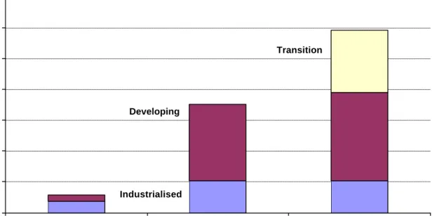
Measured by the number of crisis events worldwide, there appears to be a substantial increase in financial instability in the 1980s, with respect to the 1970s levels, particularly in emerging countries, a trend which has continued in the 1990s (see Figure 3). The latter is mainly due to the larger number of crisis which occurred in transition countries in this decade and to the additional – although marginal – increase in the number of crisis in emerging countries.

(12)

Figure 3: Distribution of crises by decades and countries

(percentage of total crises)

0 10 20 30 40 50 60 70 1970s 1980s 1990s Transition Developing Industrialised %

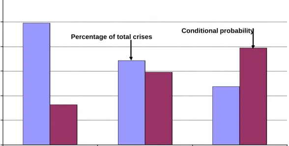
In order to assess whether the design of monetary policy can affect the likelihood of banking crisis events we conduct a few preliminary exercises before embarking in the econometric analysis. We first look at the number of crises which have occurred in the period of study (1970-2000) for each of the country groups, on the basis of their central bank objectives. Figure 4 (blue column) shows that those countries whose central bank objectives do not include price stability experienced the lowest percentage of crisis, followed by those with no statutory objectives and those whose central banks narrowly focus on price stability as single (or main) objective. On the other hand, those countries

with objectives compatible a priori with price stability have suffered the largest

percentage of crises.

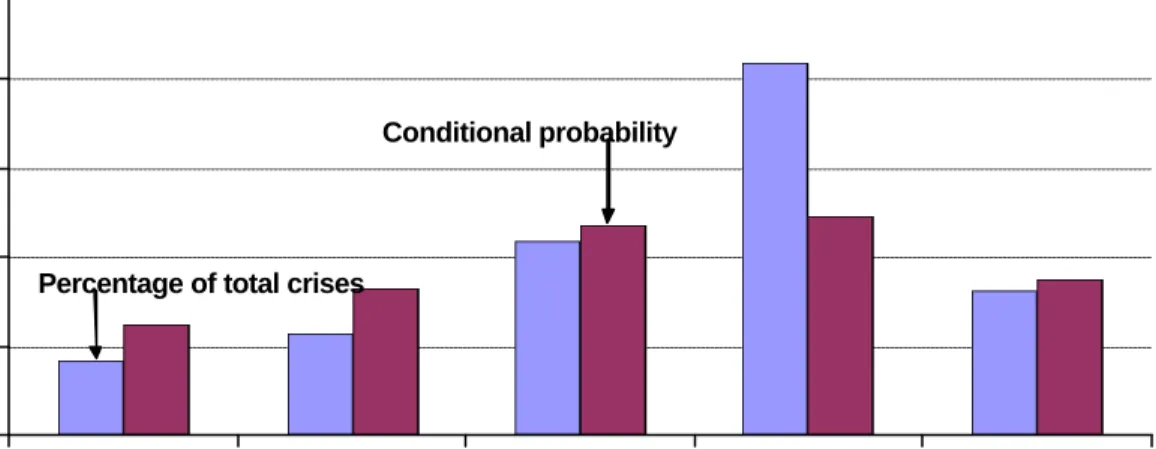
Since this stylised facts may biased by the number of observations in each group we use conditional probabilities to assess under which type of central bank objectives the probability of a banking crisis is higher (Figure 4, red column). As before, those countries with no statutory central bank objectives have the lowest probability that a banking crisis may occur, followed closely by those who narrowly focus on price stability. The highest probability of crisis is again for those countries whose central banks aim at price stability with other a priori compatible objectives.

In the same vein, we look at the number of crises which have occurred between 1970 and 2000 in each country group, classified on the basis of their monetary policy

(13)

strategies. Figure 5 (blue column) shows that countries whose central banks target the exchange rate are the ones with the highest percentage of crisis events, followed by those under monetary targeting. However, these stylised facts are clearly biased by the higher number of observations of exchange rate targeting and, to a lower extent, monetary targeting. The conditional probabilities (red column in the same Figure) actually show that the probability of a banking crisis event is clearly lower for countries whose central banks target the exchange rate, followed by monetary targeting. The highest probability is that of countries with inflation targeting.

Obviously enough, these stylised facts do not allow us to extract any definitive conclusions, since we have not take into account important factors already identified in the empirical literature as affecting the probability of a banking crisis. This will be our next step.

Figure 4: Distribution of crises by Central Bank Objectives

(percentage of total crises and conditional probability of crisis)

0 10 20 30 40 50 Other objectives without price stability

No objectives Price stability with others conflictive Price stability with others compatible Price stability major or only objective %

Percentage of total crises

(14)

Figure 5: Distribution of crises by monetary policy strategies

(percentage of total crises and conditional probability of crisis)

0 10 20 30 40 50 60

Exchange rate target Money target Inflation target

%

Percentage of total crises

Conditional probability

6. Empirical methodology

We estimate the relationship between monetary policy design and financial instability, controlling for other relevant variables. The former is defined in terms of the central bank objectives and the monetary policy strategy (exchange rate, monetary or inflation targeting) and the latter in terms of the occurrence of banking crises. The occurrence – or not – of a banking crisis is defined in terms of a dummy, which requires a binary

model of estimation. We choose a logit model to this end4.

We use a logistic distributive function to estimate whether, and to what extent, our regressors affect the probability of a banking crisis. The dependent variable equals zero in years and countries where there are no crises and it equals one in the country and year where a crisis. Given the logistic distribution, the probability of a banking crisis in period t can be expressed as follows:

) ( ) ( 1 1 ' 1 ' 1 ) | 1 ( Pr − − + = = − t t X X t e e X Crisis ob β β (1)

Similarly, the probability of no crisis in period t is:

) ( 1 1 ' 1 1 ) | 0 ( Pr − + = = ₋ t X t e X Crisis ob β (2) 4

(15)

The ratio of (1) over (2) is the odds ratio in favour of a crisis. Taking natural logs of this ratio, it should be clear that it is not only linear inXt−1, but also linear in the parameters

ß. Given (3), ß measures the change in the log-odds ratio for a unit change inXt−1 5 . 1 ' 1 1 ) | 0 ( Pr ) | 1 ( Pr ln ₋ − − ₌ = = t t t X X Crisis ob X Crisis ob _β (3)

In order to minimize that heterogeneity problem inherent in a study with 79 countries, we could have used a conditional logit (fixed effects), so as to take into account the possibility of unobservable individual fixed effects correlated with the regressors. However, this would have reduced considerably the number of observations in our panel. Even more importantly, it would have eliminated the information content of some countries that have not experienced any crisis as well as the few countries, especially transition countries, which have being in crisis during the whole sample period for which data was available for them. Also, our objective variables do not have a high degree of time variation; indeed some are drawn from surveys conduced for decades (such as Cukierman et al. 1992 for the central bank objectives). For these reasons we use random effects for estimation.

Other than the heterogeneity among countries, an additional estimation problem we face is endogeneity. Once a crisis starts it is likely to affect the evolution of the macro and financial variables and even our objective variable, the monetary policy regime. This is might be true notwithstanding the findings of the empirical literature previously reviewed that money demand continues to be stable in the long run even after a systemic banking crisis. This should reduce central bankers’ interest in changing the design of monetary policy but they could still decide to do so.

To avoid potential endogeneity, the empirical literature of banking crises only gives the value of one to the starting year of the crisis and eliminates the crisis observations beyond the first year. In addition, in order to minimize simultaneity problems all regressors are lagged one period. These two adjustments reduce the number of

5

However, the marginal effect of a regressor on the dependent variable, which is the usual interpretation for coefficients in the ordinary least squares setup, is different from ß (although it still depends on it), namely: ) exp( 1 1 ) exp( 1 ) exp( ) | 1 ( Pr 1 ' 1 ' 1 ' 1 1 − − − − − + ∗ + ∗ = ∂ = ∂ t t t t t X X X X X Crisis ob β β β β

Note that this expression will vary withX_t₋₁. In practice, the marginal effects are calculated at the means of the regressors.

(16)

observations to 1181, rather than 1492, and the number of countries to 71 (27 industrialised, 31 developing and 13 transition) instead of the original 796.

6. RESULTS

With the methodology described above, we conduct one set of regression, which can be considered the baseline, and three more sets of regressions, as robustness tests. Each set is composed of three regressions.

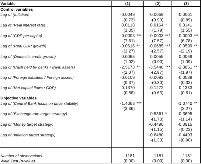
The first set – the baseline – includes all countries in the sample and takes a narrow definition of banking crisis, which only includes systemic events, as dependent variable. This should eliminate those crises stemming from one or a few banks’ mismanagement and not necessarily from macroeconomic, institutional or policy rated issues. We conduct three regressions: The first includes the central bank objectives as the single objective variable and all macroeconomic and financial variables previously described as control variables.

The results show the important role that the central bank objectives play in determining the likelihood of a banking crisis, as shown by the negative highly significant coefficient, at a 95% confidence level (see column 1 of Table 1). In particular, countries whose central banks narrowly focus on price stability appear to have a lower probability of suffering from a banking crisis, other things given. In addition, higher economic growth and higher real GDP per capita –proxing the quality of institutions - significantly reduce the probability of a banking crisis, as one would expect. Finally, more liquidity in the banks’ balance sheets, measured by the share of cash held by banks to bank assets, also appears to reduce the likelihood of a banking crisis.

The second set of regressions concentrates on the other objective variable: the monetary policy strategy. The central bank objectives are excluded to avoid any interference. The results yield a negative and significant coefficient for the exchange rate based strategy, at the 10% confidence level. In other words, among the three monetary policy strategies included (exchange rate, monetary based and inflation targeting), the former is superior as far as financial stability is concerned. Again, this is for a definition of financial stability focused on banking crisis events and not in asset

6

The eight countries lost are transition ones which had experienced crises throughout the period for which there was data for the regressors. Given that we take lags we need at least two observations to keep a country in the sample.

(17)

prices or other broader issues. As for the control variables, the results are roughly the same as in the first regression except for an additional one: higher real interest rates mildly contribute to a higher probability of crisis (column 2 of Table 1).

The third regression of the baseline exercise includes all objective variables together. While the central bank objectives continue to have a negative and highly significant coefficient, this is no longer true for the exchange rate based strategy. Therefore, the fact that countries with central bank objectives narrowly focused on price stability tend to suffer from fewer crises, other factors given, is robust to the inclusion of all objective variables. The same is true for high economic growth, GDP per capita and bank liquidity (column 3 of Table 1).

Variable

Control variables

Lag of (Inflation) -0.0049 -0.0059 -0.0061

-(0.73) -(0.90) -(0.89)

Lag of (Real interest rate) 0.0118 0.0164 * 0.0141

(1.35) (1.79) (1.55)

Lag of (GDP per capita) -0.0003 *** -0.0003 *** -0.0003 ***

-(7.61) -(7.57) -(6.78)

Lag of (Real GDP growth) -0.0616 ** -0.0685 *** -0.0599 **

-(2.27) -(2.57) -(2.19)

Lag of (Domestic credit growth) 0.0065 0.0055 0.0069

(1.02) (0.90) (1.09) Lag of (Cash held by banks / Bank assets) -2.5173 ** -3.5448 *** -2.3851 **

-(2.07) -(2.97) -(1.97) Lag of (Foreign liabilities / Foreign assets) -0.0109 -0.0083 -0.0089 -(0.37) -(0.30) -(0.32)

Lag of (Net capital flows / GDP) -0.1370 -0.1272 -0.1333

-(0.58) -(0.63) -(0.61)

Objective variables

Lag of (Central Bank focus on price stability) -1.4063 *** -1.0740 ** -(3.36) -(2.27)

Lag of (Exchange rate target strategy) -0.5361 * -0.3695

-(1.73) -(1.14)

Lag of (Money target strategy) -0.4490 -0.0915

-(1.15) -(0.22)

Lag of (Inflation target strategy) -0.6480 -0.4493

-(1.33) -(0.90)

Number of observations 1181 1181 1181

Wald Test (p-value) (0.00) (0.00) (0.00)

Note: Logit estimates with random effects. Tests: z-statistics robust to heteroskedasticity; Wald test measures the joint significance of all coefficients and it is distributed as a Chi squared with degrees of freedom equal to the number of coefficients.

Table 1: Logit Estimations for Systemic Banking Crises in All countries

This table presents the coefficients and z-statistics (in parentheses) for the logit estimations of the probability of a systemic banking crisis. *, **, and *** denote significance at 10%, 5%, and 1%, respectively.

(18)

Given that the distinction between systemic and non systemic crisis is not very systematic in the available surveys, we carry out the same regressions on a broader crisis definition. This includes both systemic and non-systemic crises as events for our binary model. The results hardly change in the three model specifications: only central bank objectives as objective variable (column 1 of Table 2), only monetary policy strategies (column 2 of Table 2) and all objective variables (column 3). The main difference is that with this broader definition of crisis, the choice of monetary policy strategy offers clearer results. In fact, an exchange rate based strategy not only reduces the likelihood of a crisis when taken as single objective variable as before, but also when including the central bank objectives as additional objective variable. The results obtained in the baseline for the control variables are maintained for a broader crisis definition: higher economic growth, per capital GDP and bank liquidity reduce the likelihood of a crisis, other things given. Finally, in the second and third specifications higher inflation appears to reduce the probability of a crisis at a 10% confidence interval. This result is in line with the recent literature strand which considers very low levels of inflation as the origin of euphoria and potential crises in countries not used to price stability. In any event, the result is not very robust, since it is not found in the baseline or in the other robustness exercises.

V a r i a b l e C o n t r o l v a r i a b l e s L a g o f ( I n f l a t i o n ) - 0 . 0 0 7 6 - 0 . 0 1 0 6 * - 0 . 0 1 0 4 * - ( 1 . 2 2 ) - ( 1 . 7 1 ) - ( 1 . 6 6 ) L a g o f ( R e a l i n t e r e s t r a t e ) 0 . 0 1 2 9 0 . 0 1 6 7 * * 0 . 0 1 4 3 * ( 1 . 5 9 ) ( 1 . 9 9 ) ( 1 . 7 4 ) L a g o f ( G D P p e r c a p i t a ) - 0 . 0 0 0 2 * * * - 0 . 0 0 0 2 * * * - 0 . 0 0 0 2 *** - ( 7 . 2 1 ) - ( 7 . 3 1 ) - ( 6 . 3 0 ) L a g o f ( R e a l G D P g r o w t h ) - 0 . 0 7 9 1 * * * - 0 . 0 7 6 3 * * * - 0 . 0 6 9 1 *** - ( 3 . 2 2 ) - ( 3 . 1 7 ) - ( 2 . 8 6 ) L a g o f ( D o m e s t i c c r e d i t g r o w t h ) 0 . 0 0 5 1 0 . 0 0 5 7 0 . 0 0 6 6 ( 0 . 9 0 ) ( 1 . 0 2 ) ( 1 . 1 6 ) L a g o f ( C a s h h e l d b y b a n k s / B a n k a s s e t s ) - 2 . 2 0 8 8 * * - 2 . 6 2 5 5 * * * - 1 . 6 8 6 1 * - ( 2 . 1 8 ) - ( 2 . 6 4 ) - ( 1 . 7 2 ) L a g o f ( F o r e i g n l i a b i l i t i e s / F o r e i g n a s s e t s ) - 0 . 0 1 3 7 - 0 . 0 1 2 0 - 0 . 0 1 2 3 - ( 0 . 4 9 ) - ( 0 . 4 5 ) - ( 0 . 4 7 ) L a g o f ( N e t c a p i t a l f l o w s / G D P ) - 0 . 0 2 4 1 - 0 . 0 7 0 6 - 0 . 0 5 4 6 - ( 0 . 1 1 ) - ( 0 . 4 2 ) - ( 0 . 3 0 ) O b j e c t i v e v a r i a b l e s L a g o f ( C e n t r a l B a n k f o c u s o n p r i c e s t a b i l i t y ) - 1 . 1 8 5 9 * * * - 0 . 8 9 1 8 *** - ( 3 . 5 6 ) - ( 2 . 5 1 ) L a g o f ( E x c h a n g e r a t e t a r g e t s t r a t e g y ) - 0 . 8 2 6 6 * * * - 0 . 6 9 5 1 *** - ( 3 . 3 7 ) - ( 2 . 7 9 ) L a g o f ( M o n e y t a r g e t s t r a t e g y ) - 0 . 1 0 6 5 0 . 0 9 4 9 - ( 0 . 3 6 ) ( 0 . 3 1 ) L a g o f ( I n f l a t i o n t a r g e t s t r a t e g y ) - 0 . 4 6 6 6 - 0 . 2 1 0 6 - ( 1 . 1 8 ) - ( 0 . 5 2 ) N u m b e r o f o b s e r v a t i o n s 1 1 1 5 1 1 1 5 1 1 1 5 W a l d T e s t ( p - v a l u e ) ( 0 . 0 0 ) ( 0 . 0 0 ) ( 0 . 0 0 ) N o t e : L o g i t e s t i m a t e s w i t h r a n d o m e f f e c t s . T e s t s : z - s t a t i s t i c s r o b u s t t o h e t e r o s k e d a s t i c i t y ; W a l d t e s t m e a s u r e s t h e j o i n t s i g n i f i c a n c e o f a l l c o e f f i c i e n t s a n d i t i s d i s t r i b u t e d a s a C h i s q u a r e d w i t h d e g r e e s o f f r e e d o m e q u a l t o t h e n u m b e r o f c o e f f i c i e n t s . T a b l e 2 : L o g i t E s t i m a t i o n s f o r S y s t e m i c a n d N o n - s y s t e m i c B a n k i n g C r i s e s i n A l l c o u n t r i e s T h i s t a b l e p r e s e n t s t h e c o e f f i c i e n t s a n d z - s t a t i s t i c s ( i n p a r e n t h e s e s ) f o r t h e l o g i t e s t i m a t i o n s o f t h e p r o b a b i l i t y o f a b a n k i n g c r i s i s . * , * * , a n d * * * d e n o t e s i g n i f i c a n c e a t 1 0 % , 5 % , a n d 1 % , r e s p e c t i v e l y . ( 1 ) ( 2 ) ( 3 )

(19)

Another important issue which might have a bearing with our empirical analysis is the location of the responsibility for banking regulation and supervision. In fact, central banks in charge of regulation and supervision may have a special interest in reducing the likelihood of a banking crisis, being an additional aim in their portfolio, other than monetary policy. We control for the location of regulation and supervision responsibilities by introducing a dummy variable which takes the value of one whe n the central bank is in charge and zero otherwise.

When including this additional variable, the central bank objectives continue to be significant – albeit mildly - in the model specification which includes both systemic and non-systemic banking crises (column 4 of Table 3,). This means that countries whose central banks narrowly focus on price stability have a lower probability of suffering from all kinds of banking crises, even when controlling for the location of bank regulation and supervision. In the same vein, having an exchange rate-based monetary policy strategy significantly reduces the likelihood of banking crisis (at a 95% confidence level), even when controlling for the location of regulation and supervision (column 5 of Table 3,). This holds true when including the central bank objectives as additional variable (column 6 or Table 3,). These results, however, do not hold any longer for a stricter definition of banking crisis, with systemic events only (column 1, 2 and 3 of Table 3). Finally, an interesting result drawn from this model specification is that locating bank regulation and supervision significantly reduces the likelihood of a banking crisis. This finding is robust to the dependent variable chosen (only systemic or all crises) and to the number of objective variables included (only central bank objectives, only monetary policy strategies, or both). It should be noted, however, that the relevance of this finding is limited by potentially large endogeneity problems. These cannot be minimized as for the other regressors because the dummy variable representing the location of regulation and supervision is time-invariant. In fact, available information does not allow to include changes in the location of responsibilities for regulation and supervision over time, even if they have taken place, and perhaps even as a consequence of a crisis.

(20)

Variable

Lag of (Inflation) -0.0001 -0.0009 -0.0013 -0.0051 -0.0075 -0.0078

(-0.02) (-0.14) (-0.21) (-0.85) (-1.22) (-1.27)

Lag of (Real interest rate) 0.0135 * 0.0155 * 0.0144 * 0.0136 * 0.0155 * 0.0139 *

(1.69) (1.88) (1.74) (1.74) (1.94) (1.75) Lag of (GDP per capita) -0.0003 *** -0.0003 *** -0.0003 *** -0.0002 *** -0.0002 *** -0.0002 ***

(-8.12) (-7.97) (-7.34) (-7.45) (-7.42) (-6.63) Lag of (Real GDP growth) -0.0521 ** -0.0527 ** -0.0506 * -0.0702 *** -0.0634 *** -0.0604 **

(-2.02) (-2.01) (-1.91) (-2.88) (-2.63) (-2.49)

Lag of (Domestic credit growth) 0.0061 0.0064 0.0068 0.0059 0.0069 0.0072

(1.03) (1.07) (1.12) (1.07) (1.26) (1.31) Lag of (Cash held by banks / Bank assets) -2.7822 *** -3.0175 *** -2.6352 ** -2.0940 ** -2.1189 ** -1.6237 *

(-2.52) (-2.85) (-2.33) (-2.16) (-2.28) (-1.72) Lag of (Foreign liabilities / Foreign assets) -0.0164 -0.0108 -0.0127 -0.0101 -0.0076 -0.0094 (-0.57) (-0.40) (-0.47) (-0.39) (-0.31) (-0.38)

Lag of (Net capital flows / GDP) -0.1418 -0.1370 -0.1381 -0.0106 -0.0579 -0.0463

(-0.58) (-0.62) (-0.60) (-0.05) (-0.32) (-0.24)

Lag of (Central Bank focus on price stability) -0.4517 -0.3440 -0.6606 * -0.5392

(-1.18) (-0.82) (-1.88) (-1.52)

Lag of (Exchange rate target strategy) -0.2475 -0.2301 -0.6468 *** -0.6008 **

(-0.84) (-0.78) (-2.64) (-2.44)

Lag of (Money target strategy) -0.1586 -0.0629 0.0895 0.1803

(-0.44) (-0.17) (0.30) (0.60)

Lag of (Inflation target strategy) -0.2848 -0.2111 -0.2313 -0.0983

(-0.63) (-0.46) (-0.60) (-0.25) Lag of (Central Bank Supervision of Financial System) -1.1626 *** -1.1669 *** -1.0980 *** -0.7986 *** -0.8233 *** -0.6960 ***

(-4.37) (-4.46) (-3.98) (-3.11) (-3.39) (-2.78)

Number of observations 1181 1181 1181 1115 1115 1115

Wald Test (p-value) (0.00) (0.00) (0.00) (0.00) (0.00) (0.00)

Table 3: Logit Estimations for Banking Crises in All countries controlling for Central Bank Supervision of Financial System.

This table presents the coefficients and z-statistics (in parentheses) for the logit estimations of the probability of a systemic banking crisis. *, **, and *** denote significance at 10%, 5%, and 1%, respectively.

Systemic Banking Crises Systemic and Non-systemic Banking Crises

Note: Logit estimates with random effects. Tests: z-statistics robust to heteroskedasticity; Wald test measures the joint significance of all coefficients and it is distributed as a Chi

(21)

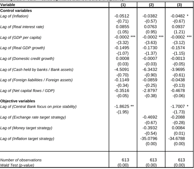
We now split the sample in three groups of countries, industrial, emerging and transition to check whether the results are robust to the different country groups. As before, in the case of industrial countries, central bank objectives focused on price stability significantly reduce the likelihood of crisis events, other variables given (column 1 of Table 4). However, no central bank strategy appears superior to the others as regards the occurrence of a banking crisis (column 2 of Table 4). When including all objective variables in the regression, having narrow central bank objectives is still significant but at a 10% degree of confidence. As for the control variables, only the real GDP per capita is found significant, with the correct sign and, in the third specification, inflation appears mildly significant with negative sign (i.e., relatively higher inflation reduces the likelihood of a crisis other things given).

Variable

Lag of (Inflation) -0.0512 -0.0382 -0.0482 *

-(0.71) -(0.57) -(0.67)

Lag of (Real interest rate) 0.0855 0.0763 0.0937

(1.05) (0.95) (1.21)

-(3.32) -(3.63) -(3.12)

Lag of (Real GDP growth) -0.1495 -0.1730 -0.1574

-(1.07) -(1.37) -(1.15)

Lag of (Domestic credit growth) 0.0008 -0.0007 -0.0013

(0.03) -(0.03) -(0.05)

Lag of (Cash held by banks / Bank assets) -4.5091 -6.3432 -3.9695

-(0.70) -(0.90) -(0.61)

Lag of (Foreign liabilities / Foreign assets) -0.1149 -0.0859 -0.0438

-(0.34) -(0.25) -(0.13)

-(0.05) -(0.38) -(0.06)

Lag of (Central Bank focus on price stability) -1.8625 ** -1.7007 *

-(1.95) -(1.73)

Lag of (Exchange rate target strategy) -0.4692 -0.2088

-(0.67) -(0.28)

Lag of (Money target strategy) -0.3932 0.0084

-(0.54) (0.01)

(0.00) (0.00)

Wald Test (p-value) (0.00) (0.00) (0.00)

Table 4: Logit Estimations for Systemic Banking Crises in Industrialised countries

This table presents the coefficients and z-statistics (in parentheses) for the logit estimations of the probability of a systemic banking crisis.*, **, and *** denote significance at 10%, 5%, and 1%, respectively.

(22)

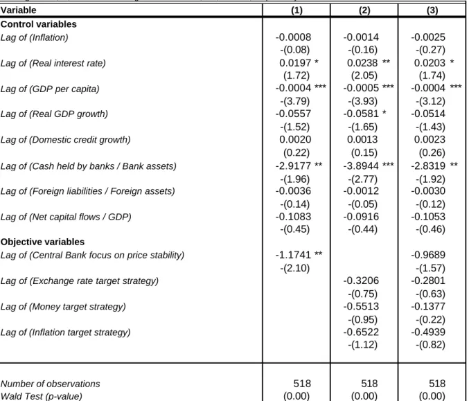
In the emerging country group the results are also similar to the baseline one (Table 5). In the first specification (which only includes central bank objectives as objective variable), countries which narrowly focus on price stability tend to suffer from fewer banking crises, other things given. In the second one, no monetary policy strategy seems superior to the others in terms of financial stability. The control variables found significant are, as in the baseline, the real interest rate, which increases the probability of a banking crises as it rises, and the real GDP per capita and the liquidity held by banks which reduce the likelihood of a banking crises.

Variable

Lag of (Inflation) -0.0008 -0.0014 -0.0025

-(0.08) -(0.16) -(0.27)

Lag of (Real interest rate) 0.0197 * 0.0238 ** 0.0203 *

(1.72) (2.05) (1.74)

-(3.79) -(3.93) -(3.12)

Lag of (Real GDP growth) -0.0557 -0.0581 * -0.0514

-(1.52) -(1.65) -(1.43)

Lag of (Domestic credit growth) 0.0020 0.0013 0.0023

(0.22) (0.15) (0.26)

Lag of (Cash held by banks / Bank assets) -2.9177 ** -3.8944 *** -2.8319 **

-(1.96) -(2.77) -(1.92)

Lag of (Foreign liabilities / Foreign assets) -0.0036 -0.0012 -0.0030

-(0.14) -(0.05) -(0.12)

-(0.45) -(0.44) -(0.46)

Lag of (Central Bank focus on price stability) -1.1741 ** -0.9689

-(2.10) -(1.57)

Lag of (Exchange rate target strategy) -0.3206 -0.2801

-(0.75) -(0.63)

-(0.95) -(0.22)

-(1.12) -(0.82)

Wald Test (p-value) (0.00) (0.00) (0.00)

Table 5: Logit Estimations for Systemic Banking Crises in Developing countries

(23)

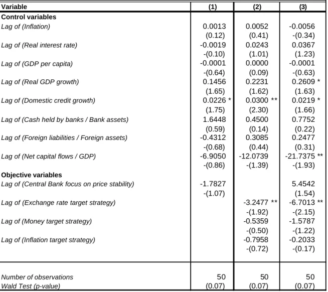
Finally, the same exercise is conducted for transition countries. This is the only case in which having central bank objectives which narrowly focus on price stability does not reduce the probability of banking crises, in a significant way. On the other hand, the choice of an exchange rate based strategy is clearly superior to the other two since it significantly reduces the likelihood of crisis both when monetary policy strategies are the single objective variable (column 2 of Table 6) and when the central bank objectives are included (column 3 of Table 6). This result could be interpreted as if for transition economies choosing the correct strategy has proven more important for financial stability than focusing on price stability, while the other is true for the full sample. It should be noted however, that the results for the transition country group should be taken with care, due to the small number of observations stemming from the structural break in the early 1990s.

Variable

Lag of (Inflation) 0.0013 0.0052 -0.0056

(0.12) (0.41) -(0.34)

Lag of (Real interest rate) -0.0019 0.0243 0.0367

-(0.10) (1.01) (1.23)

Lag of (GDP per capita) -0.0001 0.0000 -0.0001

-(0.64) (0.09) -(0.63)

Lag of (Real GDP growth) 0.1456 0.2231 0.2609 *

(1.65) (1.62) (1.63)

Lag of (Domestic credit growth) 0.0226 * 0.0300 ** 0.0219 *

(1.75) (2.30) (1.66)

Lag of (Cash held by banks / Bank assets) 1.6448 0.4500 0.7752

(0.59) (0.14) (0.22)

Lag of (Foreign liabilities / Foreign assets) -0.4312 0.3085 0.2477

-(0.68) (0.44) (0.31)

Lag of (Net capital flows / GDP) -6.9050 -12.0739 -21.7375 **

-(0.86) -(1.39) -(1.93)

Lag of (Central Bank focus on price stability) -1.7827 5.4542

-(1.07) (1.54)

Lag of (Exchange rate target strategy) -3.2477 ** -6.7013 **

-(1.92) -(2.15)

-(0.50) -(1.22)

-(0.72) -(0.17)

Wald Test (p-value) (0.07) (0.07) (0.07)

Table 6: Logit Estimations for Systemic Banking Crises in Transition countries

(24)

7. CONCLUSIONS

Building upon the existing empirical literature on the factors behind financial stability, we assess the role of monetary policy design in determining the likelihood of a banking crisis.

A sample of yearly data for 79 countries for the period 1970 to 2000 yields evidence that the choice of the central bank objectives significantly influences the probability that a banking crisis may occur. In particular, focusing the central bank objectives on price stability reduces the likelihood of a banking crisis, other things given. This result is robust to the definition of banking crisis (only systemic) and to different country groups, except for transition countries. The results for this latter group, however, should be taken with care due to the relatively small number of observations on which they are drawn.

As for the monetary policy strategy, exchange rate targeting appears to be the preferred option in terms of financial stability for several model specifications. This is so when all types of banking crises are considered (systemic or not), and for the group of transition countries but not for industrial and emerging countries. This finding would support the choice of relatively fixed exchange rate regimes in countries in transition as far as financial stability is concerned while not necessarily for other country groups.

We also control for the location of regulatory and supervisory responsibilities, being a particularly relevant variable in countries whose central banks are in charge of supervision. Even in this case focusing the central bank objectives on price stability is still superior for a broad definition of banking crises. The same is true for an exchange rate based monetary policy strategy. Finally, locating regulatory and supervisory responsibilities at the central bank reduces the likelihood of a banking crisis in all the model specifications where this variable has been included. This is a strong result for a long debated issue for which no firm empirical evidence exists. However, the result should be taken with caution because of endogeneity problems

(25)

Appendix

Data sources and definitions of variables

Below we list the variables and sources used for this study, as well as the explanation of any change we have introduced. The data is annual and it covers the period 1970-99.

Dependent variable:

* Systemic and Non-systemic banking crises dummy: equals one during episodes identified as in Caprio and Klingebiel (2003). They present information on 117 systemic banking crises (defined as much or all of bank capital being exhausted) that have occurred since the late 1970s in 93 countries and 51 smaller non-systemic banking crises in 45 countries during that period. The information on crisis is cross-checked with that of Domaç and Martinez-Peria (2000).

Source: Caprio and Klingebiel (2003) and Dolmaç and Martinez Peria (2000).

Objective variables:

* Central Bank focus on price stability: measures to what extent statutory objectives do provide the central bank with a clear focus on price stability following the approach of Cukierman et al. (1992). Statutory monetary objectives may be potentially conflicting with price stability when objectives such as employment or growth are stated separately without being qualified by statements such as “without prejudice to monetary or price stability”. Financial stability objectives are not interpreted as potentially conflicting with monetary stability. The classification of objectives varies somewhat from Cukierman’s and it is more similar to that of Mahadeva and Sterne (2000). The variable takes the following values: 0 (only goals other than price stability); 0.25 (no statutory objectives); 0.5 (price stability with other conflicting objectives); 0.75 (price stability + financial stability and non-conflicting monetary stability objectives); and 1 (only goal is price,

monetary or currency stability) 7. The list of objectives and countries is available by

decades, so we have assumed it constant through every year of each decade.

7

Cukierman’s classification distinguishes between “price stability is the only objective”, rated 0.8, and “price stability is the major or only objective in the charter, and the central bank has the final word in case of conflict with other government objectives”, rated 1.

(26)

Source: For the 1970s and the 1980s, Cukierman, Webb and Neyapti (1992) and Cukierman, Miller and Neyapti (2002). For the 1990s, Mahadeva and Sterne (2000). * Monetary policy strategies: these three variables (Exchange rate target, Money

target and Inflation target) are dummies that equal one during periods in which targets

for these variables were used according to the chronology of the Bank of England survey of monetary frameworks in Mahadeva and Sterne (2000). However, it provides a chronology of the adoption and removal of explicit targets and monitoring ranges for the exchange rate, monetary aggregates and inflation in the 1990s, so we had to complement it with information from other sources for the period before 1990. Regarding exchange rate arrangements, we use classifications of exchange rate strategies taken from Reinhart and Rogoff (2002), Kuttner and Posen (2001) and Berg, Borensztein and Mauro (2002), in the last case for Latin America countries. Data for monetary and inflation targets were complemented with the information taken from Kuttner and Posen (2001) and Carare and Stone (2003). It should be noted that some judgement has gone into the classification of regimes since it is difficult to identify their timeframes and characteristics.

Source: Mahadeva and Sterne (2000), Reinhart and Rogoff (2002), Kuttner and Posen (2001), Berg, Borensztein and Mauro (2002) and Carare and Stone (2003).

* Central Bank Supervision of Financial System: this variable is a dummy which takes the value 1 for countries where the Central Bank is responsible for the supervision of the financial system and takes 0 otherwise. This variable is not time-varyi ng; it stems from a survey conducted by the IMF in 1993 where all member countries where asked to inform of which institution was responsible for banking regulation and supervision in their respective countries. The results of the survey are shown in Tuya and Zamalloa (1994).

Source: Tuya and Zamalloa (1994).

Control variables:

Macroeconomic variables

* Inflation: percentage change in the GDP deflator. (Since the value for the 95% percentile is 106.3%, but the variance is extremely high due to several cases of hyperinflations, we have substituted all values above 150% for 150%).

(27)

* Real Interest Rate: Nominal interest rate minus inflation, calculated as the percentage change in the GDP deflator. (Since the value for the 5% percentile is –30% and for the 95% percentile is 21.2%, but the variance is extremely high, we have substituted all values above 50% for 50% and those below –50% for 50%).

Source: International Monetary Fund, International Financial Statistics. Where available, money market rate (line 60B); otherwise, the commercial bank deposit interest rate (line 60l); otherwise, a rate charged by the Central Bank to domestic banks such as the discount rate (line 60).

* Net Capital Flows to GDP: Capital Account plus Financial Account + Net Errors and Omissions.

Source: International Monetary Fund, International Financial Statistics, lines (78bcd + 78bjd +78cad).

* Real GDP per capita in 1995 US dollars: this variable is expressed in US dollars instead of PPP for reasons of data availability.

Source: The World Bank, World Tables; and EBRD, Transition Report, for some transition countries.

* Real GDP growth: percentage change in GDP Volume (1995=100).

Source: International Monetary Fund, International Financial Statistics (line 99bvp) where available; otherwise, The World Bank, World Tables; and EBRD, Transition Report, for some transition countries.

Financial variables:

* Domestic Credit growth: percentage change in Domestic credit, claims on private sector. (Since the value for the 95% percentile is 112.2%, but the variance is extremely high, we have substituted all values above 150% for 150%).

Source: International Monetary Fund, International Financial Statistics, line 32d.

* Bank Cash to total assets: Reserves of Deposit Money Banks / Assets of Deposit Money Banks.

Source: International Monetary Fund, International Financial Statistics, line 20 divided by lines (22a + 22b + 22c +22d +22f).

(28)

* Bank Foreign Liabilities to Foreign Assets: deposit money banks foreign liabilities to foreign assets.

Source: International Monetary Fund, International Financial Statistics, lines (26c+26cl) divided by line 21.

(29)

Country name Years Country name Years

Albania 1995-1998 Kenya 1975-1999

Argentina 1981-1999 Korea, Rep. 1976-1999

Armenia 1993-1999 Kyrgyz Rep. 1996-1998

Australia 1971-1999 Latvia 1994-1999 Austria 1970-1996 Lithuania 1994-1999 Bahamas 1985-1995 Macedonia 1996-1999 Barbados 1970-1995 Malaysia 1974-1999 Belgium 1975-1997 Malta 1971-1998 Bolivia 1976-1999 Mexico 1982-1999 Botswana 1976-1999 Moldova 1994-1999 Brazil 1981-1999 Mongolia 1993-1999 Bulgaria 1992-1997 Netherlands 1970-1997

Canada 1970-1999 New Zealand 1972-1999

Chile 1977-1999 Nicaragua 1988-1996

China 1985-1999 Nigeria 1977-1999

Colombia 1970-1999 Norway 1975-1999

Costa Rica 1970-1999 Paraguay 1988-1999

Croatia 1994-1998 Peru 1977-1999

Cyprus 1976-1999 Poland 1990-1999

Czech Republic 1994-1997 Portugal 1975-1999

Denmark 1975-1999 Romania 1993-1999

Ecuador 1975-1999 Russian Federation 1994-1999

Egypt, Arab Rep. 1976-1999 Singapore 1972-1999

Estonia 1993-1999 Slovak Republic 1994-1997

Finland 1975-1998 Slovenia 1993-1999

France 1975-1997 South Africa 1970-1999

Georgia 1996-1997 Spain 1975-1997

Germany 1970-1998 Sweden 1970-1999

Ghana 1971-1999 Switzerland 1977-1999

Greece 1975-1999 Tanzania 1976-1999

Honduras 1978-1997 Thailand 1976-1997

Hong Kong, China 1991-1999 Turkey 1974-1997

Hungary 1983-1997 Uganda 1981-1999

Iceland 1976-1999 Ukraine 1994-1998

Indonesia 1981-1999 United Kingdom 1970-1999

Ireland 1974-1998 United States 1970-1999

Israel 1979-1999 Uruguay 1978-1999

Italy 1970-1998 Venezuela, RB 1970-1999

Japan 1977-1999 Zambia 1985-1999

Kazakhstan 1995-1999

(30)

Country name Systemic Non-systemic Country name Systemic Non-systemic

Albania 1992- Kenya 1985-89,1992,1993-95

1996-Argentina 1980-82,1989-90,1995 Korea, Rep.

1997-Armenia 1994-96 Kyrgyz Rep. 1990s

Australia 1989-92 Latvia 1995-96,1998-99

Austria no crises no crises Lithuania 1995-96

Bahamas not in sample not in sample Macedonia 1993-94

Barbados not in sample not in sample Malaysia 1997- 1985-88

Belgium no crises no crises Malta not in sample not in sample

Bolivia 1986-87,1994- Mexico 1981-82,1994-97

Botswana 1994-95 Moldova not in sample not in sample

Brazil 1990,1994-99 Mongolia not in sample not in sample

Bulgaria 1991-97 Netherlands no crises no crises

Canada 1983-85 N e w Z e a l a n d 1987-90

Chile 1976,1981-87 Nicaragua 1988-96

China 1990s Nigeria 1990s 1997

Colombia 1982-87 Norway 1987-93

Costa Rica 1987 1994- Paraguay 1995-99

Croatia 1996 Peru 1983-90

Cyprus not in sample not in sample Poland 1990s

Czech Republic 1997- Portugal no crises no crises

D e n m a r k 1987-92 Romania

1990-Ecuador 1980-82,1996- Russian Federation 1995,1998-99

Egypt, Arab Rep. 1980-85 1991-95 Singapore 1982

Estonia 1992-95 1998 Slovak Republic

1991-Finland 1991-94 Slovenia 1992-94

France 1994-95 South Africa 1977,1989

Georgia 1991- Spain 1977-85

Germany 1978-79 S w e d e n 1990-94

Ghana 1982-89 1997- Switzerland no crises no crises

G r e e c e 1991-95 Tanzania

1988-Honduras no crises no crises Thailand

1983-87,1997-Hong Kong, China 1982-83, 1983-86,1998 Turkey 1982-85 1994

Hungary 1991-95 U g a n d a

1994-Iceland 1985-86,1993 Ukraine 1997-98

Indonesia 1992-97,1997- United Kingdom 1974-76,1984,1991,1995

Ireland no crises no crises United States 1980-83 1980-91

Israel 1977-83 Uruguay 1981-85

Italy 1990-95 Venezuela, RB 1994-99 1978,1981,1982,1985,1986

Japan 1992- Zambia 1995

Kazakhstan not in sample not in sample

Table A2: Countries and Crises Included. 1970-1999.

(31)

Variable No. Obs. Mean Std. Deviation Minimum Maximum

Crisis dummy 1492 0.23 0.42 0.00 1.00

Inflation 1492 72.64 562.01 -4.00 11750.00

Real interest rate 1492 8.62 626.98 -11680.85 14155.99

Real GDP per capita 1492 6925.07 4976.04 125.20 21487.30

Real GDP growth 1492 3.46 4.67 -38.29 52.55

Domestic credit growth 1492 87.91 800.47 -55.71 18939.19

Cash held by banks / Bank assets 1492 0.14 0.17 0.00 1.78

Foreign liabilities / Foreign assets 1492 1.88 4.26 0.00 85.25

Net capital flows / GDP 1492 0.00 0.71 -12.99 8.07

Central Bank focus on price stability 1492 0.61 0.31 0.00 1.00

Exchange rate target strategy 1492 0.60 0.49 0.00 1.00

Money target strategy 1492 0.27 0.44 0.00 1.00

Inflation target strategy 1492 0.17 0.38 0.00 1.00

Central Bank supervision 1492 0.69 0.46 0.00 1.00

Table A3: Descriptive statistics of the regression variables

Note: For an explanation on the construction and modification of the variables see main text and the description in this Appendix.

(32)

References

BERG, A., E. BORENSZTEIN and P. MAURO. (2002). “An Evaluation of Monetary Regime Options for Latin America”, IMF Working Paper WP/02/211.

BERNANKE, B. and M. GERTLER. (2000). “Monetary policy and asset price volatility”, NBER. National Bureau of Economic Research, Cambridge, Mass.

BERNANKE, B. and M. GERTLER. (1990). “Financial Fragility and Economic Performance”, Quarterly Journal of Economics, Vol. 105, No. 1, pp. 87-114

BLINDER, A. (1999). “General discussion: monetary policy and asset price volatility”, Fed of Kansas City Economic Review, 4th quarter, pp. 139-140.

BORDO, M. (1985). “Financial Crises, Banking Crises, Stock Market Crashes, and the Money Supply: Some International Evidence, 1980-1933”, in CAPIE, F. and G. WOOD, eds., “Financial Crises and the World Banking System, New York: St. Martin’s.

BORDO, M. and A. MURSHID. (2000) “Are financial crises becoming increasingly more contagious? What is the historical evidence on contagion?”, NBER. National Bureau of Economic Research, Cambridge, Mass.

BORDO, M., B. MIZRACH and A. SCHWARTZ. (1995) “Real versus pseudo-international systemic risk: some lessons from History”, NBER. National Bureau of Economic Research, Cambridge, Mass.

CALVO, G. (1997). “Capital flows and macroeconomic management: Tequila lessons” International Journal of Finance and Economics, vol. 1, no. 3.

CAPRIO, G. and D. KLINGEBIEL. (2003). “Episodes of Systemic and Borderline Financial Crises”, Dataset mimeo, The World Bank.

CARARE, A. and M. STONE. (2003). “Inflation Targeting Regimes”, IMF, WP/03/9. CROCKET, A. (2000). “In search of anchors for financial and monetary stability”, SUERF Colloquium, Vienna, April 2000.

CUKIERMAN, A. (1992). “Central Bank Strategy, Credibility and Independence: Theory and Evidence”, MIT Press.

CUKIERMAN, A., G. P. MILLER and B. NEYAPTI. (2002). “Central Bank Reform, Liberalization and Inflation in Transition Economies – an International Perspectives”, Journal of Monetary Economics, 49 (2002) 237-264.