The Economic Value of Volatility Timing with
Realized Jumps
∗
Ingmar Nolte
†Qi Xu
‡This Version: January 29, 2015
Abstract
This paper comprehensively investigates the role of realized jumps detected from high frequency data in predicting future volatility from both statistical and economic perspectives. Using seven major jump tests, we show that sepa-rating jumps from diffusion improves volatility forecasting both in-sample and out-of-sample. Moreover, we show that these statistical improvements can be translated into economic value. We find a risk-averse investor can significantly improve her portfolio performance by incorporating realized jumps into a volatil-ity timing based portfolio strategy. Our results hold true across the majorvolatil-ity of jump tests, and are robust to controlling for microstructure effects and trans-action costs.
JEL classification: C58, C53, G11
Keywords: high frequency data, jumps, nonparametric tests, asset allocation, volatility forecasting, realized volatility.
∗We thank Marcelo Fernandes, Sandra Nolte, Alessandro Palandri, and conference and seminar
participants at EEA-ESEM 2013 (Gothenburg), IFABS 2013 (Nottingham), and Warwick Business School for helpful comments.
†Accounting and Finance Department, Lancaster University Management School, Lancaster
Uni-versity, Lancaster, LA1 4YX, United Kingdom. Email: I.Nolte@lancaster.ac.uk.
‡Corresponding author: Finance Group, Warwick Business School, University of Warwick,
1
Introduction
The importance of jumps in asset pricing, option pricing, and risk management is widely recognized (Ait-Sahalia 2004). Although, resorting on jumps as a modeling device is not new, realized jumps were generally overlooked until recently. In this paper, we comprehensively investigate the role of realized jumps detected from high frequency data for the prediction of future volatility. Different from previous studies with similar focus, we not only conduct an extensive statistical evaluation of volatil-ity forecasting using all major jump tests, but also provide new economic insights in the form of whether a risk-averse investor can significantly benefit from considering realized jumps in volatility timing based portfolio allocation strategies.
The literature on this topic can be broadly categorized into two streams: The para-metric literature starting with Merton (1976) includes jump-diffusion and stochastic-volatility with jumps (SVJ) models in continuous time (Eraker, Johannes, and Polson 2003, Eraker 2004, Chernov, Gallant, Ghysels, and Tauchen 2003) and GARCH-J models in discrete time (Maheu and McCurdy 2004, Duan, Ritchken, and Sun 2006, Christoffersen, Jacobs, and Ornthanalai 2012). These parametric models are widely used in portfolio choice, option pricing, and risk management applications and the jumps introduced in models are ex ante in nature. As Backus, Chernov, and Martin (2011) admit: “jumps are usually treated as a modeling device to generate non-normal returns, which is economically meaningless per se”.
The second stream of the literature considers nonparametric approaches. Recently, many nonparametric jump tests (Barndorff-Nielsen and Shephard 2006, Andersen, Bollerslev, and Dobrev 2007, Ait-Sahalia and Jacod 2009) use high frequency data to estimate ex post realized jumps. This stream of the literature primarily focuses on issues such as why asset prices jump (e.g. macroeconomic new announcements) or how often asset prices jump (e.g. less than one per day). However, only a very few studies consider economic applications of realized jumps. We therefore aim to fill this gap between two related but different streams of literature by considering economic applications of realized jumps.
We focus on two research questions: Firstly, we are interested in whether realized jumps can forecast future volatility. We apply seven main stream nonparametric jump tests to identify realized jumps, decompose realized variance into jump and diffusion
components, and then adapt them into a forecasting framework. Our findings suggest that realized jumps do contain predictive information for future volatility for the ma-jority of jump tests both in-sample and out-of-sample. We find that jump models in general generate higher adjusted R squares and lower Mean Squared Prediction Er-rors (MSPE) compared to the benchmark model, which does not separate jumps from diffusion. Results hold true across the majority of jump specifications, and different forecasting horizons. Existing studies investigate similar issues. However, they mainly rely on one particular jump test and their results are mixed. For example, Andersen, Bollerslev, and Diebold (2007) find a negative (but insignificant) relationship between jumps and one period ahead volatility. Corsi, Pirino, and Reno (2010) on the contrary show statistically significant evidence to support a positive relationship if a modified jump test is applied. By using all major jump tests, our results contribute to the debate whether in general realized jumps help to forecast volatility.
Incorporating realized jumps into volatility forecasting require accessing intraday high frequency data and applying sophisticated nonparametric jump tests. Therefore, a natural question arises whether it is worth to estimate and use realized jumps. Even though separating jumps from diffusion improves volatility forecasting, it is interest-ing to know whether the improvement is large, and more importantly whether the improvement is economically valuable. Therefore, our second research question ex-plicitly asks whether the potential statistical forecasting improvement obtained by separating jumps from diffusion can be translated into tangible economic benefits for a risk-averse investor. We construct a mean-variance portfolio strategy based on the predicted volatility obtained from the previous step. Our findings suggest that the statistical improvements are also economically significant. Under different risk aver-sion levels and jump specifications, jump strategies can in general generate positive and statistically significant performance fees relative to the benchmark strategy. A few existing papers also consider the role of jumps in asset allocations. For example, Liu, Longstaff, and Pan (2003) provide an analytical solution to the optimal portfolio choice problem when event risk or jumps are considered. They find that jumps play an important role in determining the optimal portfolio choice. Two recent studies by Chen, Hyde, and Poon (2010) and Maheu, McCurdy, and Zhao (2012) are also close to us in considering jumps in asset allocation. However, we differ from those studies on a few aspects. Firstly, our nonparametric framework enables us to exploit the information embedded in jump variations in a model free fashion while previous papers rely on a parametric specification. Secondly, we use high frequency data to
separate the jumps and the diffusion component precisely, while they mainly rely on daily data to obtain relatively noisy proxies for jumps (i.e. large extraordinary move-ment or middle size jumps etc). The high frequency data we use also allows us to access intraday information, which is overlooked by previous studies.
We then conduct comprehensive robustness checks, and find that further controlling for market microstructure effects and transaction costs does not change our main results. We also investigate the predictive ability of realized jumps on alternative realized moments. We find that realized jumps can predict realized volatility and its signed components, but can hardly predict realized higher moments. We further show that a mean-variance portfolio strategy based on predicting positive and negative conditional volatilities separately can outperform the benchmark strategy based on predicting total volatility, and incorporating realized jumps can additionally improve economic benefits.
A few other studies are also related to ours. Firstly, our paper can be viewed as a natural extension of the stream of literature considering the economic value of volatility timing. Previous studies (Fleming, Kirby, and Ostdiek 2003, Bandi and Russell 2006, Bandi, Russell, and Zhu 2008, Liu 2009) already document that volatility timing performance can be improved by using high frequency data, optimal sampling, and optimal rebalancing frequencies. We extend the above studies by considering realized jumps. Secondly, our paper is also related to other uses of realized jumps or applications of jump tests. For example, Dumitru and Urga (2012) and Theo-dosiou and Zikes (2011) conduct comprehensive simulation studies to compare size and power of jump tests. Tauchen and Zhou (2011) and Jiang and Yao (2012) use detected realized jumps to predict bond risk premia and the cross-section of stock returns respectively. We distinguish ours from previous studies by focusing on the role of realized jumps in volatility timing.
The rest of the paper is structured as follows: Section 2 discusses the theoretical setup and the jump tests. Section 3 describes the data and methodology. Section 4 discusses empirical findings from both statistical and economic perspectives. Section 5 conducts comprehensive robustness checks. Section 6 concludes.
2
Jumps in Asset Prices
2.1
Theoretical Setup
Let pt denote the logarithmic price which follows a jump diffusion process given by
dpt=µtdt+σtdWt+dJt (1)
where µt, σt, and dWt are drift, diffusion parameter, and standard brownian motion
respectively. Jt is a jump process, and Jt =PNtj=1ctj, where ctj is the jump size and
Nt a counting process. For simplicity, we only consider finite activity jumps and we
assume that the jump and the diffusion components are independent. Let rj,t =p(t−1)h+hj
M −p(t−1)h+ h(j−1)
M
, j = 1, . . . , M,
wherehis the length of the intraday sampling interval andM is the number of intraday returns during the day. Then the realized variance can be written as the sum of the squared intraday returns
RVt=RVt,M = M X
j=1
r2j,t
Given the price dynamics of the jump diffusion process, the realized variance as an approximation to the price’s quadratic variance can be further written as follows
lim M→∞RVt,M = t Z t−1 σs2ds+ Nt X j=1 c2j (2) HereRtt−1σ2
sds is the integrated variance (IVt), and PNtj=1c2j is the quadratic variation
of the jump part (JVt) over the period from t−1 tot (often a day). Jump tests are
therefore designed to estimate JVt using high frequency data.
2.2
Jump Tests
We consider the use of seven major jump tests developed in the literature, includ-ing Barndorff-Nielsen and Shephard (2006) (BNS), Ait-Sahalia and Jacod (2009)(AJ), Jiang and Oomen (2008)(JO), Andersen, Dobrev, and Schaumburg (2012) (Med, Min), Corsi, Pirino, and Reno (2010)(CPR), and Podolskij and Ziggel (2010) (PZ). In this part, we only describe the BNS jump test in detail. Specifications of all other six tests are described in Appendix 1. Andersen, Bollerslev, and Dobrev (2007) and Lee and
Mykland (2008) are two other important tests that are however not studied in this paper.1
Barndorff-Nielsen and Shephard (2006) developed a bipower based jump estimator. The idea is using the calculated realized bipower variation to proxy the integrated variance. Since jumps are rare and are unlikely to occur for two consecutive intraday returns, when intervals are small enough, the realized bipower variation will converge in probability to the integrated variance. The difference between realized variance and realized bipower variation is then an estimator of the jump variation. The realized bipower statistic is defined as
BVt,M = µ−12M M −1 M X j=2 |rtj−1||rtj|, lim M→∞BVt,M −→IV = t Z 0 σ2 sds.
Following Huang and Tauchen (2005), the standardized BVt,M/RVt,M ratio converges
to a standard normal distribution and the test statistic is given by Jt,M = 1− BVt,MRVt,M q [(π2)2+π−5]1 Mmax(1, T Qt,M BV2 t,M) −→N(0,1), (3)
where T Qt refers to the tripower quarticity given by
T Qt,M =Mµ−4/33 M M −2 n X j=3 |rj−2|4/3|rj−1|4/3|rj|4/3, where µp =E(|U|)p =π−1/22p/2Γ(p+12 ).
The jump variation can then be obtained as
JVt = (RVt−BVt)I[Jt,M≥φ−1
α ], (4)
where the φ−1
α is the α quantile of the normal distribution.
1The reason is that both of them are intraday jump tests that average daily bipower variation to local volatility. Therefore, although they can identify which return contains a jump, they are not significantly different from BNS in volatility forecasting when only daily jump variation is considered.
3
Data and Methodology
3.1
Realized Jumps and Volatility Forecasting
We first investigate the role of realized jumps in volatility forecasting. There are many approaches to forecast volatility using high frequency data. We use the Heterogeneous Autoregressive (HAR) model of Corsi (2009) because it can be implemented easily and it can capture the long memory property of volatility processes in a straightforward way. Our benchmark model considers the use of daily, weekly, and monthly lagged realized variances to forecast one step ahead realized variance. The HAR-RV specifi-cation is as follows:
RVt,t+h−1 =β0+βRV DRVt−1 +βRV WRVt−5,t−1+βRV MRVt−22,t−1+ǫt,t+h−1. (5)
To assess the role of jumps, we consider the following HAR-RV-CJ specification: RVt,t+h−1 =β0+βIV DIVt−1+βIV WIVt−5,t−1+βIV MIVt−22,t−1+βJV DJVt−1+ǫt,t+h−1,
(6) whereRVt,t+h =h−1[RVt+RVt+1...+RVt+h−1] is the averagedh-periods realized
vari-ance. IVt−1,IVt−5,t−1,IVt−22,t−1 are jump robust integrated variation estimators over
a lagged daily, weekly, and monthly horizon,JVt−1 is the daily lagged jump variation
detected using the jump tests introduced before.
3.2
Realized Jumps and Volatility Timing Based Portfolio
Strategy
We then conduct our economic evaluations by constructing volatility timing based portfolio allocation strategies. We consider a risk-averse investor with mean-variance preferences, who allocates her wealth into one risky asset (a market index ETF) and one risk-free asset. Our one risky asset specification is similar to Marquering and Ver-beek (2004). The economic intuition for this strategy is simple. Given the expected return, when the volatility level is high, the investor allocates more wealth into the risk-free asset, and when the volatility level is low, the investor allocates more wealth into the risky asset. If separating jumps from diffusion components lead to more ac-curate prediction of future volatility, then we should expect the investor to improve her portfolio performance by actively rebalancing the portfolio based on the signal of the predicted volatility.
Although more sophisticated utility functions can be used, we stick to mean-variance preferences because we are primarily interested in whether statistical improvements in volatility forecasting by separating jumps from diffusion can be translated into eco-nomic values. To concentrate on the impact of jumps, we consider only one market index as the risky asset. We choose this setting to avoid dealing with jump tests in multivariate settings and controlling for non-synchronicity of different assets, while we still maintain the generality of our empirical results. We also assume that the investor is myopic. Namely, the investor dynamically rebalances her portfolio period by period, and she does not consider the intertemporal hedging demand in the port-folio selection. We make this assumption both for simplicity to directly translate our volatility forecasting results into portfolio performance and for consistency with the existing volatility timing literature.
Hence, the investor solves the following optimization problem: Max
wt U[Et(rp,t+1), V art(rp,t+1)],
where Et(rp,t+1) is the conditional expected portfolio return and V art(rp,t+1) is the
conditional variance of the portfolio return. The portfolio return isEt(rp,t+1) =rf,t+1+
wt(Et(rm,t+1)−rf,t+1), wherewtis the portfolio weight of the risky asset, Et(rm,t+1) is
the conditional expected return of the risky asset and rf,t+1 is the return for the risk
free asset, which we know ex ante.
The mean-variance utility function is given by
U[Et(rp,t+1), V art(rp,t+1)] =Et(rp,t+1)−
γ
2V art(rp,t+1),
with γ the risk-aversion parameter. Hence, the optimal portfolio weight is given by wt=
Et(rm,t+1)−rf,t+1
γV art(rm,t+1)
. (7)
We set the expected return for the risky asset equal to the in-sample mean 2, as over
a short horizon, expected return changes are negligible and we are only interested in the volatility timing effect of realized jumps.
Fleming, Kirby, and Ostdiek (2003) show that using a dynamic volatility timing strat-egy relying solely on realized volatilities can outperform both static strategies and dynamic volatility timing strategies using lagged daily volatilities only. Therefore 2We also tried using other specifications such as rolling windows, results are similar.
the question whether realized jumps are economically valuable can be translated into whether our jump augmented volatility timing strategy (HAR-RV-CJ) can outperform the benchmark strategy (HAR-RV) which does not separate jumps from the diffusion component.
To implement the above strategy, we conduct two further adjustments. Firstly, we impose a short selling constraint. Following Marquering and Verbeek (2004), we re-strict the negative portfolio weights to zero and the greater than one portfolio weights to one. Secondly, we also match the high frequency trading period (6.5 hour) to daily frequency (24 hour). Therefore, rather than directly plugging in the predicted realized variance, we adjust the predicted realized variance with a bias-correction factor. We follow existing studies (Fleming, Kirby, and Ostdiek 2003, Bandi and Russell 2006) and construct the bias-correction factor as follows:
BCF = 1/n
Pn t=1r2t
1/nPnt=1RVt
, (8)
whereRVtis the daily realized variance for 6.5 trading hours andrtis the daily return
for 24 hours. We construct the bias-correction factor using all data from the in-sample period. The conditional variance is estimated by predicted realized variance scaled by the bias correction factor, namely V art(rm,t+1) = BCF ·RVdt+1, where RVdt+1 is the
predicted realized variance obtained from the volatility forecasting part. We can then plug in the conditional variance into the optimal portfolio weight function to estimate the optimal portfolio weight.
3.3
Performance Evaluations
Following the volatility timing literature, we focus on the utility based performance evaluation measure to assess whether investors can benefit from including realized jumps into their information set. We follow Fleming, Kirby, and Ostdiek (2003) and Marquering and Verbeek (2004) and rely on averaged realized utility to compare jump strategies to the benchmark strategy.
The sample averaged realized utility for portfolio strategy p is given by ¯ U(Rp) = 1 T T−1 X t=0 [rp,t+1− γ 2V art(rp,t+1)]. (9)
Given the optimal portfolio weights, we can compute daily time series of ex post portfo-lio returnsrp,t+1=rf,t+1+wt(rm,t+1−rf,t+1) and variancesV art(rp,t+1) = (rp,t+1−¯rp)2,
and then plug that in to obtain the averaged realized utility.3
To quantify the economic benefit relative to the benchmark strategy, we use the per-formance fee ∆ (in basis points), which is the fee an investor is willing to pay to switch from the benchmark strategy (with portfolio returnrbm,t ) to our strategy (e.g.
strat-egy p with portfolio return rp,t). In our analysis, we consider different risk aversion
levels (γ = 2,6,10). The performance fee is computed as follows: 1 T T−1 X t=0 [(rp,t+1−∆)− γ 2V art(rp,t+1)] = 1 T T−1 X t=0 [rbm,t+1− γ 2V art(rbm,t+1)]. (10)
3.4
Statistical Significance of Economic Values
One of the major concerns of existing studies on the economic value of return/volatilty prediction is the statistical significance of the economic value obtained. The economic value computed is just a figure and usually not large (e.g in the unit of basis points), hence we don’t know whether the value is significantly different from zero across different strategies. Therefore different methods have been used to investigate the statistical significance of economic values. Following Engle and Colacito (2006) and Bandi, Russell, and Zhu (2008), we address this concern by viewing the economic gains as loss differential in which we compare one portfolio to the benchmark portfolio. The approach is in the spirit of Diebold and Mariano (1995). The Diebold-Mariano (DM) test was designed to examine whether the loss differential of two forecasts is statisti-cally significantly different from zero. The test can be used when the loss differential series is covariance stationary. Engle and Colacito (2006) and Bandi, Russell, and Zhu (2008) applied it to examine whether the ex post portfolio-volatility-difference between a candidate strategy and a benchmark strategy is statistically significantly different from zero. In our study, we investigate whether the performance fees (viewed as loss differential) are significantly different from zero. We first compute the time se-ries of daily “spot” realized utilities and then the time sese-ries of daily performance fees for each strategy in comparison to the benchmark. Afterwards, we construct the DM statistics and test whether the alternative strategies do not outperform the benchmark 3Alternatively, we can estimate the portfolio variance from the variance of the risky asset (we can use ex post realized variance scaled with the bias correction factor) scaled by the squared weight,
(null hypothesis) using a one-sided t-test with a robust variance covariance estimator.4
3.5
Data Description
In our empirical analysis we use the S&P500 ETF or SPDR contract (SPY) as the risky asset, obtained from NYSE TAQ database. The contract tracks the S&P500 index and is very liquidly traded. Trading spans from 9:30 EST to 16:00 EST. Our sample spans from Jan 2nd 2001 to Dec 31st 2010. To start with we compute the realized volatility estimator based on equidistant observations sampled at the conven-tional five minute frequency in order to control for market microstructure noise. In the robustness checks section, we also report the results of a more advanced estimator to control for market microstructure noise – the average RV estimator of Andersen, Bollerslev, Christoffersen, and Diebold (2011). This estimator is a sub-sample esti-mator that can also be constructed easily. Starting from one minute regular spaced log-returns, we compute the average RV as an equally-weighted average of five overlap-ping five minute RV estimators. Andersen, Bollerslev, and Meddahi (2011) found that the average RV estimator can perform as well as more complex estimators (realized kernel, multiple time scale, pre-averaging etc) in volatility forecasting. We implement two further adjustments: Firstly, we remove the overnight periods. Secondly, we use linear interpolation to correct for different trading hours, especially in December 2008 and afterwards. We also collect S&P500 ETF or SPDR contract (SPY) daily data from CRSP in order to match intraday trading period to daily frequency. As the risk-free asset we use the daily average of the one month US Treasury bill series.
4
Empirical Findings
4.1
Statistical Findings
This part presents volatility forecasting results using realized jumps. Table 1 docu-ments the descriptive statistics for the realized variance and realized jump variations using different jump tests. Although the statistics from different jump tests look dif-ferent, they all share the same features, including high skewness and high kurtosis, 4An alternative way to assess the statistical significance of economic gains is to use bootrapping methods. A recent study by McCracken and Valente (2013) provides a formal test of economic values using the bootstrapping method.
supporting the asymmetric and rare event nature of jumps. We first conduct in-sample statistical evaluations by estimating our models with the whole sample data from 2001 and 2010.
Table 2 shows in-sample volatility forecasting results for the benchmark model and models using different jump tests. We follow Andersen, Bollerslev, and Diebold (2007) and use the Newey-West variance covariance matrix estimator with 5, 10 and 44 lags for daily, weekly, and monthly ahead forecasts. For the benchmark HAR-RV model, the one day ahead forecast shows that only the coefficient of weekly lagged realized variance is significant at the 5% level, while for one week and one month ahead fore-casts all three lagged realized variance coefficients are significant. The adjR2 takes
values of 0.562, 0.682 and 0.644 for the different forecasting horizons. We then look at the HAR-RV-CJ models using different jump tests. At least four points are worth mentioning. Firstly, although at weekly and monthly horizons, coefficients for the integrated variances are all significant as in the benchmark model, the HAR-RV-CJ results differ from the HAR-RV model at daily horizon. While weekly and monthly lagged integrated variances remain insignificant, the daily lagged integrated variances now become significant, indicating that jump robust integrated variation is more im-portant than total realized variance in daily volatility forecasting. Secondly, the jump signs are almost all negative.5 Our result is consistent with Andersen, Bollerslev, and
Diebold (2007), but is different from Corsi, Pirino, and Reno (2010). Therefore, Corsi, Pirino, and Reno (2010)’s explanation that larger jumps lead to higher future volatil-ity due to an increased level of disagreement may not hold in our setup. Instead, our findings are more consistent with Andersen, Bollerslev, and Diebold (2007)’s explana-tion that jumps are quickly mean reverting and hence can lead to a lower volatility rather than a higher one. Thirdly, jump coefficients differ in terms of the significance. Jump coefficients are significant across all horizons for BNS, JO and PZ, significant only at daily horizon for Med, Min, CPR, and insignificant for AJ across all horizons at the 5% level. Finally, we look at the goodness-of-fit of the models. We find that almost all models with different jump specifications can outperform the benchmark HAR-RV model at all forecasting horizons. At daily level, the highest adjR2 is PZ of
0.604 and the lowest is AJ of 0.562. BNS has an adjR2 of 0.592. Compared to BNS,
CPR, JO, and Med have higher adjR2s while Min has a lower adjR2. For weekly and
monthly ahead forecasts, adjR2s are all close to 0.70 and 0.65 respectively. Although
5The exception of AJ and its later relative weak statistical performance can mainly be justified by its finite sample properties in a simulation analysis reported in the Appendix.
we observe a clear inverse U shape pattern ofadjR2s levels across forecasting horizons
for all models, the improvements in adjR2s compared to the benchmark model are
diminishing from about 3% on daily horizon to about 1% on average on weekly and monthly horizons.
Although in-sample findings document a clear improvement in volatility forecasting by separating jumps from diffusion, we are also interested in whether results hold true out-of-sample. We first estimate model parameters using the first 1000 days of the whole sample as the in-sample period, and then use the rest of the sample from 2006 to 2010 as the out-of-sample period. Table 3 reports our out-of-sample volatility forecasting results. We report the Mean Squared Error (MSE) for the predicted value compared to the realized value. Similar to the in-sample analysis, we find that all RV-CJ models using different jump tests can outperform the benchmark HAR-RV in terms of lower MSEs. This finding holds true for all daily, weekly, and monthly horizons. Similar to the in-sample findings, we observe i) the largest statistical im-provements at daily horizons and ii) imim-provements diminish when forecasting horizons increase. When we compare out-of-sample findings across different jump tests, we find that AJ has the lowest out-of-sample performance. Models using PZ, CPR, Med, or JO outperform BNS while the model using Min underperforms BNS. Results are con-sistent with in-sample findings and hold true across forecasting horizons.
4.2
Out-of-Sample Economic Findings
Given the significant statistical improvement by separating jump and diffusion com-ponents, we are now interested in whether such statistical accuracy can be translated into economic value for a risk-averse investor. We construct volatility timing strategies as discussed above for our out-of-sample period (2006 to 2010). The largest statis-tical forecasting improvement was observed for a daily horizon and given that the jump effect is quickly mean reverting we concentrate on volatility timing with daily re-balancing. To calculate the optimal portfolio weights we use the model-predicted volatility as a predictor for conditional volatility, and then adjust it with the bias-correction factor as illustrated in equation (8).
Table 4 reports the out-of-sample economic findings. Our main performance mea-sure is performance fee, interpreted as the fee that an investor is willing to pay to switch from a benchmark strategy to a jump augmented strategy. We consider three
risk aversion levels γ = 2,6,10. We show that all jump strategies generate positive performance fees in comparison to the benchmark strategy, and the economic val-ues generated depend on different jump strategies and risk aversion levels. For the moderate risk aversion level of 6, we show that highest performance fees are 20 basis points for Med and Min, followed by 19 basis points for BNS and CPR, and 18 and 17 basis points for JO and PZ. AJ generates positive but very small performance fee; a result that is consistent with its negligible forecasting improvement in the statistical part. The economic magnitude is also affected by the change of the risk aversion level, ranging from 59 basis points (γ = 2) to 11 basis points (γ = 10), indicating that the strategy seems to work better for less risk averse investors. Around 0.6% annualized performance fee looks small in magnitude, and we therefore also assess the statistical significance of the economic value generated. We find that except for AJ, all jump strategies generate positive and statistically significant performance fees with DM t-statistics above 2. To summarize, we find that the separation of jumps from diffusion components improves volatility timing strategies for almost all jump tests. The out-of-sample economic findings are generally consistent with in-sample and out-out-of-sample statistical findings, although it does not necessarily match with the ranking of the in and out-of-sample volatility forecasting analyses. One possible explanation could be that jumps not only affect the volatility process, but also the return process, which is not captured by our volatility timing strategies.
5
Robustness Checks
In this section, we conduct comprehensive robustness checks. We focus on three issues: Firstly, our main results are based on the RV estimator sampled as the conventional five minutes sampling frequency. It is interesting to see whether our results still hold true under a more stringent control of market microstructure noise. Secondly, although we show that incorporating realized jumps in volatility timing generates economic value, we are also interested in whether it is feasible for an investor to exploit this in the presence of transaction costs. Thirdly, we also discuss whether realized jumps can help to predict realized higher moments and semi-variances, and whether performances can be improved using these in the portfolio allocation. Further extensions and robustness checks including simulation analysis, good and bad jumps,
and sub-sample analysis can be found in the Appendix6.
5.1
Market Microstructure Noises
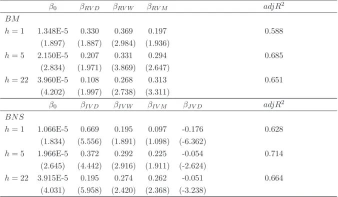
We follow Andersen, Bollerslev, Christoffersen, and Diebold (2011) and Andersen, Bollerslev, and Meddahi (2011) and construct average realized variances and bipower variations. Table 5 reports the in-sample volatility forecasting results after further controlling for market microstructure noises. Although the jump coefficient is still negative and significant as shown in Section 3.2, the adjR2 is different. For the one
day ahead forecast, the adjR2 for the benchmark model raises from 0.562 to 0.588
when using the average RV estimator. Similarly, the adjusted adjR2 for the
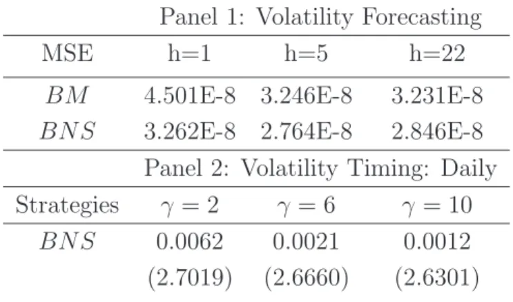
HAR-RV-CJ with BNS raises from 0.592 to 0.628. A similar statistical improvement is also found in the out-of-sample evaluation as shown in panel 1 of Table 6. Such statis-tical improvements by using subsample estimators also indicate potential economic improvements. The out-of-sample portfolio allocation results are shown in panel 2 of Table 6. We find that performance fees remain positive and statistically significant. Moreover, we show that economic magnitudes are larger using the microstructure noise robust estimators compared to the conventional five minutes estimator. A risk-averse investor is willing to pay performance fees ranging from 62 basis points (γ = 2) to 12 basis points (γ = 10) to use a jump strategy. Our findings suggest that the statistical and economic improvements by separating jumps from diffusion are not likely to be driven by market microstructure noises. Instead, we show that controlling for market microstructure noises strengthens our findings. Our results are also consistent with previous studies (Bandi and Russell 2006, Bandi, Russell, and Zhu 2008, Liu 2009) that controlling for microstructure noises improve portfolio performances.
5.2
Transaction Costs
We then analyze the impact of transaction costs on our results. Different from existing studies comparing dynamic and static strategies (Fleming, Kirby, and Ostdiek 2001) or comparing two dynamic strategies which are based on high frequency and daily information respectively (Fleming, Kirby, and Ostdiek 2003), our analysis compares two dynamic strategies both using high frequency information. Therefore, we expect that the effect of transaction costs will not be as strong as documented in the existing 6In our earlier version of the paper, we also show the results of an alternative parametric portfolio allocation strategies using realized jumps, the economic values are positive but small in magnitude and in general statistically insignificant.
literature. Following Bandi, Russell, and Zhu (2008), we define the transaction cost adjusted portfolio return in the following way:
¯
rp,t+1 =rp,t+1−ρ(1 +rp,t+1)|∆wt+1|, (11)
where ¯rp,t+1 is the transaction cost adjusted portfolio return, rp,t+1 is pre-adjusted
return, ρ is transaction cost parameter, where we choose a high value of 0.0025, cor-responding to a 2.5 cent half spread on a 10 dollar stock, ∆wt+1 is the change of the
weight from t to t+ 1, a proxy of trading turnover.
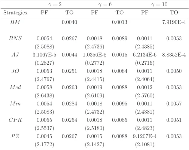
Table 7 presents the out-of-sample volatility timing results for all jump tests when transaction costs are taken into consideration. All specifications yield positive perfor-mance fees, implying that they can outperform the benchmark even when transaction costs are considered. Moreover, those performance fees are also statistically significant except for AJ. Jump strategies require incorporating recent information more quickly while the benchmark strategy is smoother, therefore we are not surprised by the higher turnover of the jump strategies compared to the benchmark strategy. Although the performance fees are slightly lower when controlling for transaction costs, we find that our results are generally consistent with our main findings in Section 4.4. Moreover, the relative performance of alternative jump specifications is also consistent with that in the main analysis, indicating that transaction costs have similar and only marginal effects for most of jump based volatility timing strategies.
5.3
Realized Jumps and Alternative Realized Moments
In practice, portfolio allocations are also subject to the impact of higher moments. Considering more general utility functions usually requires the prediction of higher moments. In addition to the sophistication of incorporating realized jumps into the portfolio allocation problem beyond mean-variance preferences, we present some sta-tistical evidence of the predictive ability of realized jumps for alternative realized mo-ments. We consider the use of realized jumps for predicting realized upside and down-side volatilities, skewness, and kurtosis. We follow Barndorff-Nielsen, Kinnebrock, and Shephard (2008) and Amaya, Christoffersen, Jacobs, and Vasquez (2013), and
construct alternative realized moments in the following way, RVt,M+ = M X j=1 rj,t2 1rj,t>0, RVt,M− = M X j=1 r2j,t1rj,t<0 RSKt,M = √ MPMj=1r3 j,t (PMj=1r2 i,t)3/2 , RKUt,M = MPMj=1r4 j,t (PMj=1r2 i,t)2
We first investigate the contemporaneous relationship between realized jumps and alternative realized moments using the following regression equation:
RMt =β0+βRJRJt+ǫt, (12)
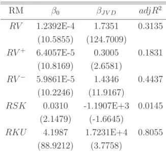
whereRMtis the realized moment including RV,RV+,RV−,RSK, andRKU. Table
8 presents the contemporaneous regression results. We find that realized jump vari-ation is a significant determinant of contemporaneous realized variance, positive and negative variances, and kurtosis, explaining 18% to 80% variation of realized moments respectively. A large jump variation is associated with a large variance, upside and downside variance, and kurtosis. Jump variation is also negatively related to realized skewness, however the relation is only marginally significant, and jumps can only ex-plain about 1% variation in skewness.
We are more interested in the predictive relationship of realized jump variation and realized moments. Therefore we forecast realized moments using daily, weekly, and monthly lagged realized moments in the fashion of the HAR model, just as we did for realized variance in Section 4.1. We consider daily, weekly, and monthly ahead forecasting horizons. The models are specified as follows:
RMt,t+h−1 =β0+βRM DRMt−1+βRM WRMt−5,t−1+βRM MRMt−22,t−1+ǫt,t+h−1. (13)
To investigate the impact of jump, we then augment the model with realized jumps. RMt,t+h−1 =β0+βRM DRMt−1+βRM WRMt−5,t−1+βRM MRMt−22,t−1+βJV DJVt−1+ǫt,t+h−1.
(14) Table 9 reports in-sample forecasting results for realized moments. The results vary across different realized moments and forecasting horizons. Firstly, we find that real-ized jump helps to forecast realreal-ized variance, even though we do not use jump robust integrated variance as we did in the main part of the analysis. For all the forecasting
horizons, we observe negative and statistically significant jump coefficients. Moreover, the adjusted R squares of the models including jumps are higher than those of the models without jumps. This finding suggests that jumps do contain incremental infor-mation for predicting future volatility and the statistical and economic improvements we documented in the main analysis do not purely come from a better measurement of jump robust integrated variance. We now discuss the role of jumps in predicting alternative realized moments: We find that realized jumps have negative and statisti-cally significant impacts on future downside volatility for all forecasting horizons and improvements in adjusted R squares range from 1% to 3%. We also find that realized jumps help to predict upside volatility at the daily horizon and generate improvements in adjusted R squares of about 0.2%. However, we show that realized jumps do not predict future realized skewness. Although realized jumps predict realized kurtosis at daily and weekly horizons, improvements in adjusted R squares are almost negligible. These results, suggest that realized jumps may not contain predictive information be-yond second moments at least in our empirical setups.
We then consider a simple portfolio allocation within the mean variance framework to quantify the predictive ability of realized jumps on alternative realized moments. We focus on upside and downside volatilities. Since the optimal portfolio weight is a function of the conditional variance of the risky asset, we can decompose it, as:
V art(rm,t+1) =V art(rm,t+1)++V art(rm,t+1)−=BCF( ˆRV +
t,t+1+ ˆRV
−
t,t+1). (15)
Since jumps have different predictive abilities to forecast upside and downside volatil-ities, an investor may improve portfolio performances by forecasting RV+t,t+1 and RV−t,t+1 separately and combining and scaling them by the Bias Correction Factor to obtain the total conditional varianceV art(rm,t+1), which can then be plugged into
the portfolio weights function as shown in equation (7). We construct two portfolio strategies: The first strategy is based on predicting upside and downside volatilities with their lagged values in the HAR fashion. To improve forecasting performance, we include both upside and downside components at daily, weekly, and monthly lagged levels to predict each component one day ahead.
RVt,t++h−1 =β0+βRV P DRVt+−1+βRV M DRVt−−1+βRV P WRVt+−5,t−1+βRV M WRVt−−5,t−1
+βRV P MRVt+−22,t−1+βRV M MRVt−−22,t−1+ǫt,t+h−1, (16)
RVt,t−+h−1 =β0+βRV P DRVt+−1+βRV M DRVt−−1+βRV P WRVt+−5,t−1+βRV M WRVt−−5,t−1
The second strategy augments the first strategy with daily lagged realized jump vari-ation as additional regressor.
RVt,t++h−1 =β0+βRV P DRVt+−1+βRV M DRVt−−1+βRV P WRVt+−5,t−1+βRV M WRVt−−5,t−1
+βRV P MRVt+−22,t−1+βRV M MRVt−−22,t−1 +βJV DJVt−1+ǫt,t+h−1, (18)
RVt,t−+h−1 =β0+βRV P DRVt+−1+βRV M DRVt−−1+βRV P WRVt+−5,t−1+βRV M WRVt−−5,t−1
+βRV P MRVt+−22,t−1+βRV M MRVt−−22,t−1 +βJV DJVt−1+ǫt,t+h−1. (19)
We focus on out-of-sample performances and consider three comparisons. The first comparison is between the first strategy based on equations (16) and (17) and the benchmark strategy in the main analysis, which predicts the total variance using HAR-RV in equation (5). The purpose is to assess whether predicting each volatility component separately can be economically valuable in comparison to predicting the total volatility. The second comparison is between the second strategy using jumps in equations (18) and (19) and the benchmark strategy in equation (5). The third comparison is between the first and second strategies, showing whether jumps con-vey incremental economic improvements. Table 10 reports out-of-sample portfolio performance fees for those three cases. We find that strategies based on predicting each volatility component separately outperform the benchmark strategy based on predicting total volatility, and can generate positive and statistically significant eco-nomic values. To be specific, in the first comparison, if we only use lagged upside and downside volatilities, we can generate annualized performance fees ranging from 13 basis points (γ = 2) to 2 basis points (γ = 10). If we include realized jumps, then the performance fees increase to range from 45 basis points (γ = 2) to 8 basis points (γ = 10). The third comparison suggests that including jump is important and can generate incremental economic improvements from 31 basis points (γ = 2) to 6 basis points (γ = 10) .
To summarize, we show that jumps do contain incremental predictive information for future volatility and its signed components, however realized jumps can hardly predict future realized higher moments. Therefore, the results suggest that realized jumps do not contribute much to moment timing based portfolio strategies beyond mean-variance approaches. If we remain in the mean-variance framework, predicting positive and negative volatility components separately can generate tangible economic improvements compared to predicting total volatility, and incorporating jumps can further improve the magnitude of the economic value.
6
Conclusion
Although a number of different nonparametric jump tests were developed in the lit-erature, only very few studies analyze the potential use of realized jumps. Using high frequency data and seven major nonparametric jump tests, this paper investigates the predictive information content of realized jumps on volatility timing from both statistical and economic perspectives.
Covering all major jump tests, we confirm that separating jumps from the diffusion component does improve volatility forecasting in general. The result holds true both in-sample and out-of-sample. Moreover, we show that using a simple volatility timing strategy, a risk-averse investor can generate a significant economic value by separating jumps from the diffusion component. We conduct comprehensive robustness checks. We show that after controlling for microstructure noise and transaction costs, our main results still hold. We also find that realized jumps can predict realized volatility and its signed up and down components, and portfolio performance can be improved by separately predicting each component.
Our paper contributes to the field on a few aspects: Firstly, we contribute to the existing literature on the role of jumps in volatility forecasting. By using seven dif-ferent jump tests, we show that jumps in general help to forecast volatility. Secondly, we show that the statistical improvement can also be exploited in a mean-variance portfolio allocation strategy. Hence, we also contribute to the literature on economic value of volatility timing. Thirdly, we contribute to the literature on the use of high frequency data and nonparametric jump tests. Our study can be viewed as evaluations of alternative jump tests using real world data while most previous studies focus on simulations. Further extensions include dealing with multivariate jumps (co-jumps), using more sophisticated utility functions, and considering alternative economic ap-plications. They are beyond the purpose of our paper, and we leave them to future studies.
References
Ait-Sahalia, Y.(2004): “Disentangling diffusion from jumps,”Journal of Financial Economics, 74(3), 487–528.
Ait-Sahalia, Y.,andJ. Jacod(2009): “Testing for Jumps in a Discretely Observed Process,”Annal of Statistics, 37(1), 184–222.
Amaya, D., P. Christoffersen, K. Jacobs, and A. Vasquez (2013): “Does Realized Skewness Predict the Cross-Section of Equity Returns?,” Creates research papers, School of Economics and Management, University of Aarhus.
Andersen, T. G., T. Bollerslev, P. F. Christoffersen,and F. X. Diebold
(2011): “Financial Risk Measurement for Financial Risk Management,” Creates research papers, School of Economics and Management, University of Aarhus.
Andersen, T. G., T. Bollerslev, and F. X. Diebold (2007): “Roughing It Up: Including Jump Components in the Measurement, Modeling, and Forecasting of Return Volatility,”The Review of Economics and Statistics, 89(4), 701–720.
Andersen, T. G., T. Bollerslev, and D. Dobrev (2007): “No-arbitrage semi-martingale restrictions for continuous-time volatility models subject to leverage effects, jumps and i.i.d. noise: Theory and testable distributional implications,”
Journal of Econometrics, 138(1), 125–180.
Andersen, T. G., T. Bollerslev, and N. Meddahi (2011): “Realized volatility forecasting and market microstructure noise,”Journal of Econometrics, 160(1), 220– 234.
Andersen, T. G., D. Dobrev, and E. Schaumburg (2012): “Jump-Robust Volatility Estimation using Nearest Neighbor Truncation,”Journal of Econometrics, 169(1), 75–93.
Backus, D., M. Chernov, and I. Martin (2011): “Disasters Implied by Equity Index Options,”Journal of Finance, 66(6), 1969–2012.
Bandi, F., J. Russell, and Y. Zhu (2008): “Using High-Frequency Data in Dy-namic Portfolio Choice,”Econometric Reviews, 27(1-3), 163–198.
Bandi, F. M., and J. R. Russell (2006): “Separating microstructure noise from volatility,”Journal of Financial Economics, 79(3), 655–692.
Barndorff-Nielsen, O. E., S. Kinnebrock, and N. Shephard (2008): “Mea-suring downside risk — realised semivariance,” Creates research papers, School of Economics and Management, University of Aarhus.
Barndorff-Nielsen, O. E., and N. Shephard(2004): “Power and Bipower Vari-ation with Stochastic Volatility and Jumps,”Journal of Financial Econometrics, 2(1), 1–37.
(2006): “Impact of jumps on returns and realised variances: econometric analysis of time-deformed Levy processes,”Journal of Econometrics, 131(1-2), 217– 252.
Chen, K., S. Hyde, and S.-H. Poon (2010): “Economic Implications of Extraor-dinary Movements in Stock Markets,” Working paper, University of Manchester.
Chernov, M., R. Gallant, E. Ghysels, and G. Tauchen(2003): “Alternative models for stock price dynamics,”Journal of Econometrics, 116(1-2), 225–257.
Christoffersen, P., K. Jacobs, and C. Ornthanalai (2012): “Dynamicjump-intensities and risk premiums: Evidence from S&P500 returns and options,”Journal of Financial Economics, 106(3), 447–472.
Corsi, F. (2009): “A Simple Approximate Long-Memory Model of Realized Volatil-ity,”Journal of Financial Econometrics, 7(2), 174–196.
Corsi, F., D. Pirino, and R. Reno (2010): “Threshold bipower variation and the impact of jumps on volatility forecasting,” Journal of Econometrics, 159(2), 276–288.
Diebold, F. X., and R. S. Mariano (1995): “Comparing Predictive Accuracy,”
Journal of Business & Economic Statistics, 13(3), 253–63.
Duan, J.-C., P. Ritchken, and Z. Sun (2006): “Approximating Garch-Jump Models, Jump-Diffusion Processes, And Option Pricing,” Mathematical Finance, 16(1), 21–52.
Dumitru, A., andG. Urga(2012): “Identifying Jumps in Financial Assets: a Com-parison between Nonparametric Jump Tests,”Journal of Business and Economic Statistics, 30(02), 242–255.
Engle, R. F., and R. Colacito (2006): “Testing and Valuing Dynamic Cor-relations for Asset Allocation,”Journal of Business and Economic Statistics, 24, 238–253.
Eraker, B. (2004): “Do Stock Prices and Volatility Jump? Reconciling Evidence from Spot and Option Prices,”Journal of Finance, 59(3), 1367–1404.
Eraker, B., M. Johannes, and N. Polson (2003): “The Impact of Jumps in Volatility and Returns,”Journal of Finance, 58(3), 1269–1300.
Fleming, J., C. Kirby, andB. Ostdiek(2001): “The Economic Value of Volatility Timing,”Journal of Finance, 56(1), 329–352.
(2003): “The Economic Value of Volatility Timing Using “Realized Volatil-ity”,”Journal of Financial Economics, 67(3), 473–509.
Huang, X., and G. Tauchen(2005): “The Relative Contribution of Jumps to Total Price Variance,”Journal of Financial Econometrics, 3(4), 456–499.
Jiang, G., and T. Yao (2012): “Stock Price Jumps and Cross-Sectional Return Predictability,”Journal of Financial and Quantitative Analysis, p. forthcoming.
Jiang, G. J., and R. C. Oomen (2008): “Testing for jumps when asset prices are observed with noise-a “swap variance” approach,”Journal of Econometrics, 144(2), 352–370.
Lee, S. S., and P. A. Mykland(2008): “Jumps in Financial Markets: A New Non-parametric Test and Jump Dynamics,”Review of Financial Studies, 21(6), 2535– 2563.
Liu, J., F. A. Longstaff, and J. Pan (2003): “Dynamic Asset Allocation with Event Risk,”Journal of Finance, 58(1), 231–259.
Liu, Q. (2009): “On portfolio optimization: How and when do we benefit from high-frequency data?,”Journal of Applied Econometrics, 24(4), 560–582.
Maheu, J. M., and T. H. McCurdy (2004): “News Arrival, Jump Dynamics, and Volatility Components for Individual Stock Returns,” Journal of Finance, 59(2), 755–793.
Maheu, J. M., T. H. McCurdy, and X. Zhao(2012): “Do Jumps Contribute to the Dynamics of the Equity Premium?,” Working paper, University of Toronto.
Marquering, W., and M. Verbeek (2004): “The Economic Value of Predicting Stock Index Returns and Volatility,”Journal of Financial and Quantitative Analy-sis, 39(02), 407–429.
McCracken, M., and G. Valente (2013): “Testing Economic Value of Asset Return Predictability,” working paper, Federal Reserve Bank of St. Louis.
Merton, R. C. (1976): “Option pricing when underlying stock returns are discon-tinuous,”Journal of Financial Economics, 3(1-2), 125–144.
Patton, A., and K. Sheppard (2011): “Good Volatility, Bad Volatility: Signed Jumps and the Persistence of Volatility,” working paper, Duke University.
Podolskij, M., and D. Ziggel (2010): “New tests for jumps in semimartingale models,”Statistical Inference for Stochastic Processes, 13(1), 15–41.
Tauchen, G., and H. Zhou (2011): “Realized jumps on financial markets and predicting credit spreads,”Journal of Econometrics, 160(1), 102–118.
Theodosiou, M., andF. Zikes(2011): “A Comprehensive Comparison of Nonpara-metric Tests for Jumps in Asset Prices,” Working paper, Imerial College London.
Tables
Table 1: Descriptive Statistics
RV JVBN S JVAJ JVJO JVM ed JVM in JVCP R JVP Z
Mean1.324E-4 4.693E-6 1.313E-6 4.919E-6 6.377E-6 5.906E-6 8.223E-6 6.855E-6 Std 3.109E-4 7.692E-5 1.748E-5 7.689E-5 9.836E-5 9.805E-5 1.042E-4 7.836E-5 Skew 10.321 43.829 40.756 43.881 42.242 43.188 40.479 41.555 Kurt 158.187 2.056E+3 1.867E+3 2.060E+3 1.945E+3 2.040E+3 1.827E+3 1.906E+3
Min 3.468E-6 0 0 0 0 0 0 0
Max 0.0065 0.0037 8.131E-4 0.0037 0.0046 0.0046 0.0048 0.0037 Notes: The table summarizes the main descriptive statistics. We report realized variance (RV), and realized jump variations for seven different jump tests (BNS, AJ, JO, Med, Min, CPR, PZ). The sample period spans from Jan 1st 2001 to Dec 31st 2010. Both realized variance and realized jump variations are computed as shown in Section 2 using the 5 minutes high frequency Spyder contract (SPY) tracking the S&P500 index.
Table 2: In-Sample Volatility Forecasting Results RVt,t+h−1 =β0+βRV DRVt−1+βRV WRVt−5,t−1+βRV MRVt−22,t−1+ǫt,t+h−1 RVt,t+h−1 =β0+βIV DIVt−1+βIDWIVt−5,t−1+βIV MIVt−22,t−1+βJV DJVt−1+ǫt+h−1 β0 βRV D βRV W βRV M adjR2 BM h= 1 1.436E-5 0.278 0.425 0.187 0.562 (1.953) (1.887) (4.115) (1.767) h= 5 2.204E-5 0.180 0.370 0.282 0.682 (2.779) (2.029) (4.643) (2.568) h= 22 4.103E-5 0.092 0.290 0.303 0.644 (4.249) (2.211) (2.951) (3.401) β0 βIV D βIV W βIV M βJV D adjR2 BN S h= 1 1.601E-5 0.467 0.325 0.132 -0.359 0.592 (2.548) (3.897) (3.745) (1.372) (-4.121) h= 5 2.354E-5 0.279 0.335 0.242 -0.158 0.699 (3.130) (3.197) (3.840) (2.143) (-2.451) h= 22 4.223E-5 0.145 0.284 0.275 -0.097 0.654 (4.256) (4.390) (3.840) (2.855) (-2.001) AJ h= 1 1.362E-5 0.280 0.419 0.188 2.931 0.562 (1.845) (1.883) (4.061) (1.791) (1.641) h= 5 1.991E-5 0.177 0.369 0.276 6.662 0.693 (2.436) (2.038) (4.544) (2.471) (1.608) h= 22 3.996E-5 0.091 0.290 0.299 3.599 0.648 (4.261) (2.213) (2.944) (3.306) (1.647) JO h= 1 1.532E-5 0.466 0.338 0.128 -0.366 0.593 (2.503) (3.848) (3.958) (1.349) (-4.093) h= 5 2.306E-5 0.287 0.337 0.239 -0.195 0.702 (3.173) (3.161) (4.039) (2.175) (-2.936) h= 22 4.187E-5 0.147 0.281 0.279 -0.099 0.654 (4.219) (4.418) (2.806) (2.920) (-2.258) M ed h= 1 1.594E-5 0.489 0.321 0.124 -0.214 0.597 (2.576) (4.040) (1.283) (1.283) (-5.021)
β0 βIV D βIV W βIV M βJV D adjR2 h= 5 2.368E-5 0.297 0.313 0.254 -0.062 0.697 (3.181) (3.022) (2.358) (2.358) (-1.712) h= 22 4.224E-5 0.146 0.280 0.285 -0.018 0.652 (4.253) (4.365) (2.962) (2.962) (-0.362) M in h= 1 1.670E-5 0.464 0.337 0.121 -0.162 0.592 (2.664) (3.887) (3.894) (1.283) (-3.046) h= 5 2.431E-5 0.275 0.352 0.228 -0.049 0.699 (3.262) (3.174) (3.971) (2.010) (-1.355) h= 22 4.307E-5 0.143 0.294 0.265 -0.024 0.653 (4.261) (4.569) (2.817) (2.748) (-0.617) CP R h= 1 1.725E-5 0.509 0.319 0.108 -0.188 0.598 (2.838) (4.019) (3.402) (1.133) (-3.836) h= 5 2.490E-5 0.311 0.324 0.232 -0.070 0.702 (3.334) (3.327) (3.580) (2.057) (-1.849) h= 22 4.333E-5 0.154 0.285 0.272 -0.021 0.653 (4.276) (4.932) (2.807) (2.787) (-0.505) P Z h= 1 1.665E-5 0.537 0.316 0.095 -0.498 0.604 (2.884) (4.311) (3.500) (1.052) (-4.035) h= 5 2.406E-5 0.320 0.336 0.219 -0.248 0.705 (3.319) (3.306) (3.717) (2.001) (-2.481) h= 22 4.268E-5 0.165 0.288 0.263 -0.133 0.655 (4.261 (4.781) (2.776) (2.621) (-3.403)
Notes: The table reports in-sample volatility forecasting results for the SPY contract from 2001 to 2010 using different jump test. The HAR-RV model is used as the benchmark model. The HAR-RV-CJ models use realized jump variation detected using different jump tests: BNS, AJ, JO, Med, Min, CPR, and PZ. We forecast one day, one week, and one month ahead realized variances. The figures in parentheses are t-statistics computed using Newey-West corrected standard error for autocorrelation orders 5, 10, and 44 respectively. The adjR2 is the adjusted R square.
Table 3: Out-of-Sample Volatility Forecasting Results
MSE h=1 h=5 h=22
BM 5.657E-8 3.532E-8 3.504E-8 BNS 4.830E-8 3.195E-8 3.268E-8 AJ 5.656E-8 3.517E-8 3.483E-8 JO 4.794E-8 3.150E-8 3.273E-8 Med 4.733E-8 3.219E-8 3.258E-8 Min 4.881E-8 3.179E-8 3.238E-8 CP R 4.653E-8 3.107E-8 3.222E-8 P Z 4.523E-8 3.017E-8 3.214E-8
Notes: The table reports out-of-sample volatility forecasting results for the SPY con-tract for 2006 to 2010 using alternative jump tests. The HAR-RV model is used as the benchmark model. The HAR-RV-CJ model use realized jump variation detected using different jump tests: BNS, AJ, JO, Med, Min, CPR, and PZ. The out-of-sample period ranges from 2006 to 2010. We report the Mean Squared Error (MSE) for predicted volatility over one day, one week, and one month forecasting horizons.
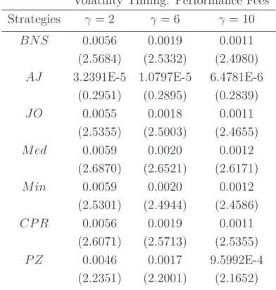
Table 4: Out-of-Sample Portfolio Performance: Daily Rebalancing Volatility Timing: Performance Fees
Strategies γ = 2 γ= 6 γ = 10 BNS 0.0056 0.0019 0.0011 (2.5684) (2.5332) (2.4980) AJ 3.2391E-5 1.0797E-5 6.4781E-6
(0.2951) (0.2895) (0.2839) JO 0.0055 0.0018 0.0011 (2.5355) (2.5003) (2.4655) Med 0.0059 0.0020 0.0012 (2.6870) (2.6521) (2.6171) Min 0.0059 0.0020 0.0012 (2.5301) (2.4944) (2.4586) CP R 0.0056 0.0019 0.0011 (2.6071) (2.5713) (2.5355) P Z 0.0046 0.0017 9.5992E-4 (2.2351) (2.2001) (2.1652)
Notes: The table reports out-of-sample portfolio allocation results for the SPY con-tract for 2006 to 2010 using alternative jump tests. The benchmark strategy uses the HAR-RV model to predict one day ahead volatility, other strategies using HAR-RV-CJ models with realized jump variation detected from the respective jump tests. We report performance fees relative to the benchmark strategy under risk aversion levels of 2, 6, and 10. Figures in parentheses are t-statistics for the DM test, where under the null hypothesis it is assumed that the (mean) performance fee equals zero.
Table 5: In-Sample Volatility Forecasting: Average RV RVt,t+h−1 =β0+βRV DRVt−1+βRV WRVt−5,t−1+βRV MRVt−22,t−1+ǫt,t+h−1 RVt,t+h−1 =β0+βIV DIVt−1+βIDWIVt−5,t−1+βIV MIVt−22,t−1+βJV DJVt−1+ǫt+h−1 β0 βRV D βRV W βRV M adjR2 BM h= 1 1.348E-5 0.330 0.369 0.197 0.588 (1.897) (1.887) (2.984) (1.936) h= 5 2.150E-5 0.207 0.331 0.294 0.685 (2.834) (1.971) (3.869) (2.647) h= 22 3.960E-5 0.108 0.268 0.313 0.651 (4.202) (1.997) (2.738) (3.311) β0 βIV D βIV W βIV M βJV D adjR2 BN S h= 1 1.066E-5 0.669 0.195 0.097 -0.176 0.628 (1.834) (5.556) (1.891) (1.098) (-6.362) h= 5 1.966E-5 0.372 0.292 0.225 -0.054 0.714 (2.645) (4.442) (2.916) (1.911) (-2.624) h= 22 3.915E-5 0.195 0.274 0.262 -0.051 0.664 (4.031) (5.958) (2.420) (2.368) (-3.238)
Notes: The table reports in-sample volatility forecasting results for the SPY contract from 2001 to 2010 controlling for market microstructure noises. The HAR-RV model and the HAR-RV-CJ model using a BNS jump test are applied to forecast one day, one week, and one month ahead realized variances. The average realized variance is used in order to control for market microstructure noise. The figures in parentheses are t-statistics using Newey-West standard errors for autocorrelation orders of 5, 10, and 44. adjR2 is the adjusted R square.
Table 6: Out-of-Sample Statistical and Economic Performances: Average RV Panel 1: Volatility Forecasting
MSE h=1 h=5 h=22
BM 4.501E-8 3.246E-8 3.231E-8 BNS 3.262E-8 2.764E-8 2.846E-8 Panel 2: Volatility Timing: Daily Strategies γ = 2 γ = 6 γ = 10
BNS 0.0062 0.0021 0.0012 (2.7019) (2.6660) (2.6301)
Notes: The table reports out-of-sample statistical and economic performances from 2006 to 2010 after controlling for market microstructure noises. Average realized variance, integrated variance, and jump variation are used to control for market mi-crostructure noise. Panel 1 reports out-of-sample volatility forecasting results. The HAR-RV model is used as the benchmark model. The HAR-RV-CJ model using a BNS jumps is also used. We report the Mean Squared Error for predicted volatility over one day, one week, and one month forecasting horizons. Panel 2 reports out-of-sample volatility timing results using the average RV estimator. Parameters are all estimated in-sample (2001-2005) and out-of-sample volatility forecasting and volatility timing are conducted out-of-sample (2006-2010). We report performance fees relative to the benchmark strategy under risk aversion levels of 2, 6, and 10. Figures in parentheses are t-statistics for the DM test, where under the null hypothesis it is assumed that the (mean) performance fee equals zero.
Table 7: Out-of-Sample Portfolio Allocation with Transaction Costs γ = 2 γ = 6 γ = 10 Strategies PF TO PF TO PF TO BM 0.0040 0.0013 7.9190E-4 BNS 0.0054 0.0267 0.0018 0.0089 0.0011 0.0053 (2.5088) (2.4736) (2.4385)
AJ 3.1067E-5 0.0044 1.0356E-5 0.0015 6.2134E-6 8.8352E-4 (0.2827) (0.2772) (0.2716) JO 0.0053 0.0251 0.0018 0.0084 0.0011 0.0050 (2.4767) (2.4415) (2.4064) Med 0.0058 0.0263 0.0019 0.0088 0.0012 0.0053 (2.6438) (2.6109) (2.5760) Min 0.0054 0.0284 0.0018 0.0095 0.0011 0.0057 (2.5083) (2.4732) (2.4381) CP R 0.0055 0.0254 0.0018 0.0085 0.0011 0.0051 (2.5537) (2.5180) (2.4823) P Z 0.0045 0.0267 0.0015 0.0088 9.1207E-4 0.0053 (2.1772) (2.1427) (2.1081)
Notes: The table reports out-of-sample portfolio allocation results for the SPY con-tract for 2006 to 2010 controlling for transaction costs. The parameters are estimated in-sample from 2001 to 2005 and the ex post portfolio returns are obtained out-of-sample (2006 to 2010). We report performance fees (PF) and turnovers (TO) for risk aversion level of 2, 6, and 10. Figures in parentheses are t-statistics for the DM test. The test has the null hypothesis that the (mean) performance fee equals to zero. TO is the mean value of the absolute change of portfolio weight.
Table 8: Contemporaneous Regressions of Realized Jumps RMt=β0+βJV DJVt+ǫt RM β0 βJV D adjR2 RV 1.2392E-4 1.7351 0.3135 (10.5855) (124.7009) RV+ 6.4057E-5 0.3005 0.1831 (10.8169) (2.6581) RV− 5.9861E-5 1.4346 0.4437 (10.2246) (11.9167) RSK 0.0310 -1.1907E+3 0.0145 (2.1479) (-1.6645) RKU 4.1987 1.7231E+4 0.8055 (88.9212) (3.7758)
Notes: This table reports the coefficients of the contemporaneous regressions of real-ized moments includingRV,RV+,RV−, RSK,RKU on realized jumps for the SPY contract for 2001 to 2010 using the BNS jump test. adjR2 is the adjusted R square
Table 9: Realized Moments Forecasting RMt,t+h−1 =β0+βRM DRMt−1+βRM WRMt−5,t−1+βRM MRMt−22,t−1+ǫt,t+h−1 RMt,t+h−1 =β0+βRM DRMt−1+βRM WRMt−5,t−1+βRM MRMt−22,t−1+βJV DJVt−1+ǫt+h−1 β0 βRM D βRM W βRM M βJV D adjR2 RV h= 1 1.436E-5 0.278 0.425 0.187 0.562 (1.923) (1.887) (4.115) (1.767) 1.518E-5 0.485 0.286 0.147 -0.914 0.591 (2.4670) (4.012) (3.549) (1.659) (-4.687) h= 5 2.204E-5 0.180 0.370 0.282 0.682 (2.568) (1.872) (4.137) (2.413) 2.252E-5 0.301 0.289 0.258 -0.536 0.697 (2.760) (2.966) (3.247) (2.340) (-3.292) h= 22 4.103E-5 0.092 0.290 0.303 0.644 (6.329) (1.675) (2.903) (2.898) 4.133E-5 0.167 0.239 0.288 -0.333 0.651 (6.318) (2.784) (2.383) (2.765) (-3.086) RV+ h= 1 6.326E-6 0.289 0.454 0.159 0.604 (1.923) (2.628) (3.714) (1.420) 6.634E-6 0.308 0.442 0.156 -.0.108 0.606 (2.047) (2.716) (3.589) (1.399) (-2.545) h= 5 9.825E-6 0.186 0.411 0.252 0.717 (2.481) (2.336) (4.089) (2.087) 9.914E-6 0.191 0.408 0.251 -0.031 0.717 (2.511) (2.329) (4.028) (2.078) (-0.913) h= 22 1.873E-5 0.098 0.301 0.310 0.668 (4.129) (4.149) (2.896) (3.059) 1.879E-5 0.102 0.299 0.309 -0.023 0.668 (4.139) (4.228) (2.903) (3.039) (-1.209)
β0 βRM D βRM W βRM M βJV D adjR2 RV− h= 1 1.030E-6 0.134 0.411 0.299 0.387 (2.072) (0.984) (3.493) (2.133) 1.035E-5 0.401 0.268 0.221 -0.647 0.419 (2.616) (3.299) (2.814) (2.352) (-3.501) h= 5 1.402E-5 0.103 0.321 0.365 0.583 (2.959) (1.253) (3.007) (2.932) 1.405E-5 0.286 0.222 0.311 -0.445 0.609 (3.378) (3.062) (2.050) (3.233) (-3.110) h= 22 2.362E-5 0.053 0.252 0.335 0.594 (4.113) (1.287) (2.307) (3.845) 2.364E-5 0.172 0.188 0.301 -0.289 0.609 (4.212) (2.638) (1.602) (4.224) (-2.725) RSK h= 1 0.027 -0.029 -0.087 0.050 0.003 (1.697) (-1.424) (-1.601) (0.422) 0.028 -0.030 -0.086 0.049 -102.129 0.003 (1.739) (-1.442) (-1.59) (0.413) (-1.188) h= 5 0.027 -0.004 -0.100 0.079 0.013 (1.908) (-0.457) (-2.283) (0.746) 0.027 -0.004 -0.099 0.078 -42.374 0.013 (1.927) (-0.519) (-2.287) (0.742) (-0.950) h= 22 0.026 -0.002 -0.010 0.023 0.027 (1.924) (-0.843) (-0.496) (0.225) 0.026 -0.002 -0.010 0.023 3.862 0.027 (1.918) (-0.825) (-0.497) (0.225) (0.429) RKU h= 1 3.333 -0.002 0.071 0.153 0.735 (7.858) (-0.120) (1.289) (1.533) 3.290 0.012 0.071 0.150 -925.924 0.735 (7.608) (0.550) (1.300) (1.513) (-2.190) h= 5 3.245 0.007 0.021 0.214 0.926 (9.464) (0.602) (0.335) (2.382) 3.213 0.018 0.021 0.217 -686.931 0.926 (9.351) (1.448) (0.337) (2.353) (-2.516) h= 22 3.378 -0.002 0.013 0.201 0.980 (12.221) (-0.345) (0.519) (2.842)
3.374 -1.081E-4 0.013 0.201 -88.993 0.980 (12.073) (-0.020) (0.519) (2.849) (-0.558)
Notes: The table reports in-sample RM forecasting results for the SPY contract from 2001 to 2010. RV, RV+, RV−, RSK, RKU are RMs used. For each RM forecasting, the HAR-RM model using its own daily, weekly, and monthly lagged RM, and the HAR-RM-J model using also the jump variation from the BNS jump test are applied to obtain one day, one week, and one month ahead forecasts. The figures in parentheses are t-statistics using Newey-West standard errors for autocorrelation orders of 5, 10, and 44 respectively. The adjR2 is adjusted R square.
Table 10: Out-of-Sample Portfolio Performance: Alternative Realized Moments Moment Timing: Performance Fees
Strategies γ = 2 γ = 6 γ = 10 RM 0.0013 4.4101E-4 2.6401E-4 (2.0816) (2.0566) (2.0316) RM +JV 0.0045 0.0015 8.9427E-4 (2.1240) (2.0899) (2.0588) JV 0.0031 0.0010 6.2967E-4 (1.7982) (1.7688) (1.7355)
Notes: The table reports out-of-sample portfolio allocation results for the SPY con-tract for 2006 to 2010 by predicting upside and downside volatilities. The first case compares portfolio performances between predicting upside and downside volatilities and predicting total realized volatility. The second case compares portfolio perfor-mances between predicting upside and downside volatilities with their past values and jumps and predicting total realized volatility. The third case compares predicting upside and downside volatilities with their past values and jumps. We report per-formance fees relative to the benchmark strategy under risk aversion levels of 2, 6, and 10. Figures in parentheses are t-statistics for DM test. The test has the null hypothesis that the (mean) performance fee equals to zero.
Online Appendix
A
Appendix 1: Jump Tests
In this part, we discuss specifications of six alternative jump tests, including Ait-Sahalia and Jacod (2009)(AJ), Jiang and Oomen (2008)(JO), Andersen, Dobrev, and Schaumburg (2012) (Med, Min) Corsi, Pirino, and Reno (2010)(CPR), and Podolskij and Ziggel (2010) (PZ).
A.1
AJ
Ait-Sahalia and Jacod (2009) find that realized power variation is invariant to different sampling scales when jumps are present. Therefore the AJ test detects the presence of jumps using the ratio of realized power variation sampled from two scales. For the realized power variation for the sampling scale h and kh with scalark >0 we have
P Vt,M(p, h) = M/hX j=1 |rj|p,and ˆ St(p, k, h) = ˆ P Vt,M(p, kh) ˆ P Vt,M(p, h) . Then the test statistic is given by
AJt,M = ˆ St(p, k, h)−kp/2−1 q ˆ Vt,M −→N(0,1), (20)
where ˆVt,M is the asymptotic variance ofSt(p, k, h). ˆ Vt,M = N(p, k) ˆAt,M(2p) MAˆt,M(p) , N(p, k) = (1/µ2p)(kp−2(1 +k))µ2p+kp−2(k−1)µ2p−2kp/2−1µk,p, µk,p=E(|U|p|U+ √ k−1V|p), ˆ At,M(2p)= (1/M) 1−p/2 µp M X j=1 |rtj|pI|rtj|<α(1/M)ω.
U,V are random variables thatU ∼N(0,1) andV ∼N(0,1) andp,k,α,ω are parameters.
A.2
JO
The swap variance test developed by Jiang and Oomen (2008) is in the spirit of Neuberger (1994)’s replicating strategy on the payoff of the variance swap contract. Different from
the other tests, which generate jump robust estimators, the JO test constructs a jump sensitive estimator. The difference between simple returns Rtj and logarithmic returnsrtj can capture one half of the integrated variance if there is no jump in the underlying sample path. Therefore the difference between twice the return difference and the realized variance can capture the jump component if a jump occurs.
SwVt,M = 2 M
X
j=1
(Rtj −rtj). Hence the test statistic using the ratio ofSwVt,M and RVt,M is
JOt,M = M BVt,M √ ΩSwV (1− RVt,M SwVt,M )−→N(0,1), (21)
where ΩSwV is the asymptotic variance using estimated integrated sixicity. ΩSwV = µ6 9 M3µ−p 6/p (M−p−1) MX−p j=0 Y k= 1p|rtj|6/p. p= 4 or 6 are suggested parameters.
A.3
Med and Min
Andersen, Dobrev, and Schaumburg (2012) introduced two simple to implement but powerful estimators for integrated variance, which use nearest neighbour truncation to control for the impact of market microstructure noise and zero returns.
M inRVt= π π−2 m m−1 m X j=2 min(|rj|,|rj−1|)2, (22) M edRVt= π 6−4√3 +π m m−2 m X j=3 med(|rj|,|rj−1|,|rj−2|)2 (23)
The statistics are as follows,
1−M inRVtRVt 1.81δmax(1,M inRQtM inRV2
t )
−→N(0,1), (24)
1− M edRVtRVt 0.96δmax(1,M edRVM edRQt2
t )
−→N(0,1), (25)
where M inRQt, M edRQt are minimum and median realized quarticity to estimate the in-tegrated quarticity. The specifications are as follow
M inRQt= πm 3π−8 m m−1 m X j=2 min(|rj|,|rj−1|)4, (26) M edRQt= 3πm 9π+ 72−52√3 m m−2 m X j=3 (|rj||rj−1||rj−2|)4. (27)
A.4
CPR
A recent study by Corsi, Pirino, and Reno (2010) extended the multipower variation in the spirit of BNS by incorporating a threshold. The idea is that large returns can result in an underrejection of jumps using multipower variation based tests. Therefore by introducing a local variance based threshold to filter out large returns, the test expects to reduce the bias. The corrected realized threshold bipower variation and corrected threshold tripower quarticity are as follows,
ctBVt,M = π 2 M X j=2 Z1(rtj, θtj)Z1(rtj−1, θtj−1), ctT Qt,M =µ−4/33 M X j=3 Z1(rtj, θtj)Z1(rtj−1, θtj−1)Z1(rtj−2, θtj−2),
where µ4/3 = E(|U|)4/3, U ∼ N(0,1), and θtj = c2θVˆtj, cθ is constant, and ˆVtj is local volatility. Z1(rtj, θtj) is the threshold function given by,
Z1(rtj, θtj) = |rtj| r2tj < θtj, 1.094θtj1/2 r2tj > θtj The statistic is as follows
1−ctBVt,M/RVt p (π2/4 +π−5)hmax(1, ctBV t,M/c