CCSO Centre for Economic Research
University of Groningen
CCSO Working Papers
July, 2005
CCSO Working paper 2005/06
Currency crises in Asia: A multivariate logit approach
Jan P.A.M. Jacobs
Faculty of Economics, University of Groningen
Gerard H. Kuper
Faculty of Economics, University of Groningen
Lestano
Currency crises in Asia:
A multivariate logit approach
∗
Jan P.A.M. Jacobs
†, Gerard H. Kuper and Lestano
Department of Economics, University of GroningenThis version: July 2005
Abstract
Indicators of financial crisis generally do not have a good track record. This paper presents an early warning system (EWS) for six countries in Asia in which indicators do work. Our binary choice model, which has been estimated for the period 1970:01–2001.12, has the following features. We extract a full list of currency crisis indicators from the literature, apply factor analysis to combine the indicators, and intro-duce dynamics. The quality of the EWS is assessed both in-sample and out-of-sample. We find that money growth (M1 and M2), na-tional savings, and import growth correlate with currency crises.
Keywords: financial crises, currency crises, early warning system, panel data, multivariate logit, factor analysis
JEL-code: C33, C35, F31, F34, F47
∗The support of the Universitas Catholic Indonesia Atma Jaya is gratefully
acknowl-edged. The present version of the paper benefited from discussions with Mardi Dungey, helpful suggestions from Marcel Fratzscher, Niels Hermes and Elmer Sterken, and com-ments received at the NAKE Research Day, Amsterdam, October 2002, the SOM Brown Bag Seminar, University of Groningen, November 2002, the Workshop on Southeast Asia, University of Groningen, May 2003, and the NAKE Research Day, De Nederlandsche Bank, Amsterdam, October 2003.
†Correspondence to: Jan P.A.M. Jacobs, Department of Economics, University of
Groningen, PO Box 800, 9700 AV Groningen, the Netherlands. Tel.: +31 50 363 3681. Fax: +31 50 363 7337. Email: j.p.a.m.jacobs@rug.nl
1
Introduction
Four waves of financial crises have hit international capital markets during the 1990s: the European Monetary System (ERM) crisis in 1992-1993, the collapse of the Mexican peso with ‘tequila effects’ in 1994-1995, the Asian flu of 1997-1998, and the Russia virus in 1998. These financial crises stimulated theoretical models and empirical analyses on their causes, impact and policy implications. Drawing lessons from these events is essential for the design of new international strategies to avoid future financial crises and to strengthen the international financial structure.
In view of the large costs associated with financial crises the question of how to predict a crisis is crucial. In addition, market indicators of default and currency risks, such as interest rate spreads and changes in credit ratings, hardly provide advance warning of financial crises. This resulted in the con-struction of a monitoring tool, the so-called early warning system (EWS).1 An EWS consists of a precise definition of a crisis and a mechanism for gen-erating predictions of crises. Typically, an EWS has an empirical structure that forecasts the likelihood of a financial crisis with indicators that show a country’s vulnerability to a crisis. EWS models differ widely in terms of the definition of financial crisis, the time span on which the EWS is esti-mated and forecast horizon, the selection of indicators, and the statistical or econometric method. A common feature of all existing EWS studies is the use of fundamental determinants of the domestic and external sectors as explanatory variables.
1For example, the IMF has put a lot of effort in EWS models, see Evans et al. (2000),
The list of studies on EWS of financial crises is long. A full list is be-yond the scope of this paper. The literature distinguishes three varieties of financial crises: currency crises, banking crises, and debt crises. Interested readers are referred to Kaminsky, Lizondo and Reinhart (1998) for papers on currency crises prior to the East Asian crisis; Bustelo (2000) and Bukart and Coudert (2002) on the East Asian crisis; and Abiad (2003) for recent studies. Gonzalez-Hermosillo (1996) and Dermirg¨u¸c-Kunt and Detragiache (1997) fo-cus on banking crises, while Cline (1995) and Marchesi (2003) survey debt crisis. We restrict our attention in this paper to currency crises.2
Several methods have been suggested for EWS models. The most pop-ular one is used in this paper, namely qualitative response (logit or probit) models. Examples are Frankel and Rose (1996) and Frankel and Wei (2005), who study currency crises and Dermirg¨u¸c-Kunt and Detragiache (1997, 2000) and Eichengreen and Arteta (2002) on banking crises. Alternatives are cross-country regression models with dummy variables as put forward by Sachs, Tornell and Velasco (1996), graphical event studies as suggested by Eichengreen, Rose and Wyplosz (1995) and Aziz, Caramazza and Saldago (2000) and the signal extraction approach, a probabilistic model proposed by Kaminsky, Lizondo and Reinhart (1998), Goldstein, Kaminsky and Rehart (2000) and Edison (2003). In the last method values of individual in-dicators are compared between crisis periods and tranquil periods. If the value of an indicator exceeds a threshold, it signals an impending crisis. Re-cently, Martinez-Peria (2002), Abiad (2003), and Chauvet and Dong (2004)
2Lestano, Jacobs and Kuper (2003) also present early warning systems for bank and
proposed a Markov-switching early warning system.
This paper develops an econometric EWS for six Asian countries, Malaysia, Indonesia, Philippines, Singapore, South Korea and Thailand. These coun-tries have been selected because the Asian flu hit Thailand and spread to other countries in the region—except Singapore—almost instantaneously. We set up logit models for currency crises with indicators extracted from a broad set of potentially relevant financial crisis indicators. The models are estimated using panel data for the January 1970–December 2001 period.
The set-up of our EWS is similar to Kamin, Schindler and Samuel (2001) and Bussiere and Fratzscher (2001), who also adopt a binomial multivari-ate qualitative response approach. However, while the final result of their (unreported) specification search is combinations of indicators as explana-tory variables, we apply factor analysis to reduce the information set. An additional novelty of our model is that we do not only include the level of the factors, but also the change therein.3 The development of the factors over time has important consequences for the probability of a currency crisis to occur. The factor analysis outcomes in combination with the estimation results and the ex post and ex ante track record allow the general conclusion that (some) indicators of financial crises do work, at least in our EWS of Asia. This finding is in contrast with IMF (2002) and Edison (2003), who conclude that the performance of EWS is generally poor and at best mixed. Our method—the combination of factor analysis and logit modeling—enables us to answer the question posed by Bustelo (2000) whether additional
indica-3Recently, Cippollini and Kapetanios (2003, 2005) and Chauvet and Dong (2004)
tors have explanatory power for financial crises. It also allows the dismissal of uninformative indicators.
The organization of the paper is as follows. Section 2 describes how we date currency crises. The results—dummy variables indicating dates of various crises—are used in binary choice models that explain the probability of crises. Section 3 describes our set of indicators, while Section 4 presents factor analysis and factors. Section 5 presents the binomial multivariate logit models for currency crises. We analyze the performance of the models in-sample and out-of-sample in Section 6. Section 7 concludes.
2
Dating currency crises
Generally, a currency crisis is defined to occur if an index of currency pres-sure exceeds a threshold.4 Eichengreen, Rose and Wyplosz (1995) made an important early effort to develop a method to measure currency pressure and to date currency crises. Their definition of exchange rate pressure is inspired by the monetary model of Girton and Roper (1977). The exchange rate is under pressure if the value of a constructed index exceeds a certain threshold. The index consists of weighted relative changes of the nominal exchange rate, international reserves and interest rates to capture successful
4Alternatives to dating schemes with thresholds are event based methods or Markov
switching models. Event based methods are commonly used in the contagion literature to date crisis from high volatility exchange rate events or news recorded by newspapers and journals, academic reviews and reports of international organizations. Examples of the former are Granger, Huang, and Yang (2000) and Ito and Hashimoto (2002); Kaminsky and Schmukler (1999), Glick and Rose (1999) and Dungey and Martin (2004) use news based currency crises. Martinez-Peria (2002), Abiad (2003) and Chauvet and Dong (2004) adopt a Markov switching framework in their EWS model, which yields currency crisis dates.
as well as unsuccessful speculative attacks. All variables in their index are relative to a reference country and their threshold is time-independent. For the dating of currency crises they set the exchange market pressure index threshold to two standard deviations from the mean. The method of Eichen-green et al. was heavily criticized which led to alternatives based on the same methodology. Kaminsky, Lizondo and Reinhart (1998) and Kaminsky and Reinhart (1999) followed the concept of Eichengreen et al. fairly closely, but they excluded interest rate differentials in their index and comparisons to a reference country. In this paper we identify episodes of currency crisis in East Asia with our own version of Kaminsky, Lizondo and Reinhart in which we include interest rates in the index. This choice is based on a more extensive evaluation of currency crises dating methods (Lestano and Jacobs, 2004). In addition, experimentation with different currency crisis concepts revealed that the concept used here performed best in an in-sample signal extraction experiment (Jacobs, Kuper and Lestano (2004)).
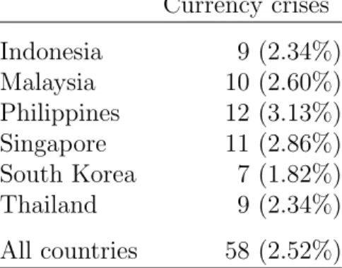
Table 1 summarizes the distribution of the currency crises over the six Asian countries in our sample. The total number of currency crises identified with our method is 58 (2.52 percent of the sample observations), distributed more or less evenly over the six countries.
[Table 1 about here.]
3
Indicators
This study focuses on indicators of macroeconomic development and external shocks. Worsening of these indicators affects the stability of financial system
and may result in a financial crisis. The indicators are selected on the basis of economic theory and recent findings of empirical studies on financial crises. See Jacobs, Kuper and Lestano (2005) for details and references. Another major consideration was the data availability on a monthly basis for our country coverage and sample. For convenience, the indicators are clustered into four major groups:
• External: Real exchange rates (REX), export growth (EXG), import growth (IMP), terms of trade (TOT), ratio of the current account to GDP (CAY), the ratio of M2 to foreign exchange reserves (MFR) and growth of foreign exchange reserves (GFR).
• Financial: M1 and M2 growth (GM1 and GM2), M2 money multiplier (MMM), the ratio of domestic credit to GDP (DCY), excess real M1 balances (ERM), domestic real interest rate (RIR), lending and deposit rate spread (LDS), commercial bank deposits (CBD), and the ratio of bank reserves to bank assets (RRA).
• Domestic (real and public): The ratio of fiscal balance to GDP (FBY), the ratio of public debt to GDP (FBY), growth of industrial production (GIP), changes in stock prices (CSP), inflation rate (INR), GDP per capita (YPC), and growth of national saving (NSR).
• Global: Growth of world oil prices (WOP), US interest rate (USI), and OECD GDP growth (ICY).
The main source of all data is the International Financial Statistics of the IMF for the macroeconomic and financial indicators and the World Bank
Development Indicators for the debt variables. We use monthly data, cover-ing six Asian countries, Indonesia, Malaysia, Philippines, Scover-ingapore, South Korea and Thailand, from January 1977 to the end of 2001. Missing data are supplemented from Thompson Datastream and various reports of the countries’ central banks. All data in local currency units are converted into US dollars. Some annual indicators are interpolated to obtain a complete monthly database.
The Appendix lists definitions, sources and transformations of our crises indicators. Two types of transformations are applied to make sure that the indicators are free from seasonal effects and stationary, 12-months percentage changes and deviation from linear trends. In case the indicator has no visible seasonal pattern and is non-trending, its level form is maintained. Some unavailable indicators are proxied by closely related indicators, for example OECD GDP is substituted by industrial production of industrial countries.
4
Factor analysis
As already mentioned in the Introduction, the aim of this paper is to cal-culate the probability of a currency crisis. However, the set of economic indicators that is informative on whether or not a crises will occur is huge. It is not feasible to include all indicators in the logit model because of too few observations and multicollinearity among the indicators. So, for each country we reduce the information set into a limited number of factors using factor analysis. These factors are then used as explanatory variables in the logit model.
Technically speaking, factor analysis transforms a set of random variables linearly and orthogonally into new random variables.5 The first factor is the normalized linear combination of the original set of random variables with maximum variance; the second factor is the normalized linear combination with maximum variance of all linear combinations uncorrelated with the first factor; and so on. By construction factors are uncorrelated. The eigenvalue for a given factor measures the variance in all the variables which is accounted for by that factor. A factor with a low eigenvalue may be ignored, because other factors are more important in explaining the variance in the set of variables under consideration.
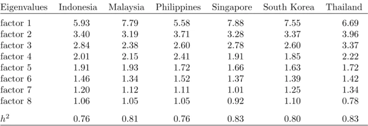
Unfortunately, there is no “best” criterion for dropping the least impor-tant factors. The so-called Kaiser criterion drops all factors with eigenvalues below one. The Cattell scree test is a graphical method in which the eigen-values are plotted on the vertical axis and the factors on the horizontal axis. The test suggests to select the number of factors that corresponds to the place of the curve where the smooth decrease of eigenvalues appears to level off to the right of the plot. In general, the scree test provides a lower bound on the number of relevant factors. In this paper we use the Kaiser criterion. Table 2 lists eigenvalues and the total variance explained by the factors for each country. For most countries, eight factors emerge with an eigenvalue above unity.6
[Table 2 about here.]
5For a detailed exposition of factor analysis including references seee.g., Venables and
Ripley (2002, Chapter 11).
6For Singapore and Thailand we maintain eight factors although only seven factors
5
Logit model
Since our dependent variable is a binary variable (where 0=no crisis and 1=crisis) we use a binary choice model. Two popular versions are the probit and the logit model. The major difference is that the probit model is based on the normal distribution, whereas the logit model uses an S-shaped logistic function to constrain the probabilities to the [0,1] interval. Predicted prob-abilities calculated by these models differ only slightly in practice. We opt for the logit model
P =F(Z) = 1 1 +e−Z =
1 1 +e−(α+βX),
where P is the probability that Z takes the value 1 and F is the cumulative logistic probability function; X is the set of regressors and α and β are parameters. It can be shown that the regression equation is equal to
ln P 1−P =Z =α+βX.
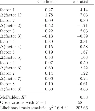
In our model, the vector of explanatory variables X consists of the eight factors rather than the full list of economic indicators themselves. However since the change in the factors may affect the probability of a currency crisis to occur, we also include differences in the factors which reduces the number of observations for each country by one. Finally, testing for fixed effects rejects the null of common effects in all models except the ERW and FR types of currency models. The results are presented in Table 3. Intercepts and country-specific intercepts (fixed effects) are not reported.
[Table 3 about here.]
From the likelihood ratio statistics, which test the joint null hypothesis that all slopes coefficient except the constant are equal to zero, we conclude that the explanatory variables (factors in levels and in differences) contribute significantly to the explanation of the variation in the crises dummies. Also, tests whether the first differences of the factors contribute significantly to the explanation of the variation in the crises dummies (not reported), leads us to conclude that this indeed is the case. In addition, we observe that factor 1 has the largest impact on the predicted probability of a currency crises; it is significantly different from zero at the 1% level. In addition, the first difference of factor 8 is significant at 1%.
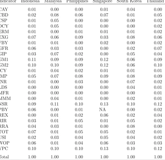
Factor 1 has by far the largest contribution to predicting crises probabil-ities. Although interpretation of the estimated coefficients in terms of the underlying indicators is not trivial, the eigenvector of factor 1 is informative, since factor 1 is a linear combination of the indicators with weights given by the first eigenvector. These weights are presented in Table 4. The largest weights in factor 1 are related to the growth of money (M1 and M2), sup-porting Kamin, Schindler and Samuel (2001),the growth of national saving, the rate of growth of GDP per capita, and import growth. These variables are dominant for all countries in our sample. Other variables that have an impact in some countries are commercial bank deposits, growth of foreign ex-change reserves, export growth, and to a lesser extent domestic real interest rate, terms of trade, and growth of world oil prices.
6
Performance
The logit models discussed above produce estimated probabilities of crises. High probabilities signal crises, low probabilities tranquil periods. The model might give false signals, i.e., a crisis does not take place despite the logit model producing a high probability. There are four possibilities. A model may indicate a crisis (high estimated probability) when a crisis indeed oc-curs (P(1,1)) or it may indicate a crisis when no crisis actually takes place (P(1,0)). It is also possible that the model does not signal a crisis (low estimated probability) where in fact a crisis does occur (P(0,1)). The final possibility (P(0,0)) is a situation in which the model does not predict a crisis and no crisis occurs. Table 5 lists the four possibilities.
[Table 5 about here.]
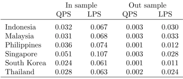
Once we generate time series of crisis probabilities, we can evaluate the forecasting ability of the model. Instead of carrying out a standard signaling experiment along the lines of e.g. Frankel and Rose (1996) and Berg and Pattillo (1999) which both require an ad-hoc assumption on the translation of estimated crisis probabilities into crisis dummies, we use the quadratic probability score (QP S) and the log probability score (LP S) proposed by Diebold and Rudebusch (1989). Both scores give an indication of the average closeness of the predicted probabilities and the observed realizations, as mea-sured by a dummy variable that takes on a value of one when there is a crisis and zero otherwise. Let Pt is the prediction probability of the occurrence of crisis or no crisis event by the model at date t and Rt is zero-one dummy
variable, that is equal to 1 if the event occurs in the actual data and equal to zero otherwise. The QPS and LPS are then given by
QP S = 1 T T X t=1 2(Pt−Rt)2 LP S = −1 T T X t=1 ((1−Rt) ln(1−Pt) +Rtln(Pt)).
The QP S ranges from 0 to 2, with a score of 0 corresponding to perfect accuracy. The LP S takes value between zero and infinity, with 0 being perfect accuracy.
We evaluate in-sample (1970.01–2001.12) and out-of-sample (2002.01– 2002.12) crisis probabilities. Table 6 reports the accuracy of the model. The second and the third column report in-sample performance, while the last two columns examine out-of-sample forecast performance. Recall that the closer the score statistics in Table 6 are to zero, the more accurate the forecasts. For all countries, the model performs quite well in-sample, except for Singapore with an LP S score of 0.11. The out-of-sample forecasts are significantly better than the in-sample projections. This should not come as a complete surprise considering the fact that hardly any currency crisis occur in the forecast period.
7
Conclusion
This paper builds an econometric EWS of six Asian countries, Malaysia, Indonesia, Philippines, Singapore, South Korea and Thailand. We set up a qualitative choice—in our case logit—model. From the literature we extract a broad set of potentially relevant financial crisis indicators which are combined into factors using factor analysis. These factors are used as explanatory variables in a panel covering the period January 1970–December 2001.
The factor analysis outcomes in combination with the estimation results of the logit model and the in-sample and out-of-sample performance allow the general conclusion that (some) indicators of financial crises do work, at least in our EWS of six Asia countries. We find that the growth rates of money (M1 and M2), GDP per capita, national savings, and imports correlate with currency crises. Other variables that have an impact in some countries are growth rates of commercial bank deposits, foreign exchange reserves, exports, and to a lesser extent domestic real interest rates, terms of trade, and world oil prices changes. So, our method—the combination of factor analysis and logit modeling—offers a solution to the bad performance (mixed and weak in timing of crisis) of EWS as noted by IMF (2002) and Edison (2003). A second, important conclusion is that first differences in indicators add to explaining probabilities of currency crises. Including dynamics in the fac-tors improves the fit of EWS models making it a more powerful surveillance instrument for policy makers.
An early warning system provides insights into which variables signal the likelihood of countries experiencing a financial crisis. The models should be
used with care though. Applying our EWS to developed economies could easily produce a result similar to what The Economist (2003) reported, the US being at risk according to Damocles, Lehman Brothers’ EWS (Subbara-man, Jones, and Shiraishi, 2003). To avoid pitfalls like these, EWS analyses should be accompanied by country risk assessments.
Appendix. Explanatory variables
Indicator Code Definition and source Transformation
External sector (current account)
Real
ex-change rate
REX Nominal exchange rate is local currency unit (LCU) per USD, IFS-AE. The CPI is IFS-64. The real exchange rate is the ratio of foreign (US CPI) to domestic prices (measured in the same currency). Thus, REX = ePf/P, where e =
nom-inal exchange rate, P = domestic price (CPI), andPf = foreign price (US CPI). A
decline in the real exchange rate denotes a real appreciation of the LCU.
Deviation from trend
Export growth
EXG IFS-70.D 12 month
percentage change Import
growth
IMP IFS-71.D 12 month
percentage change)
Terms of
trade
TOT Unit value of exports divided by the unit value of imports. Unit value of exports is IFS-74.D. Import unit value for coun-try (IFS-75.D) is not available, instead ex-ports prices of industrialized countries is used, IFS-110.74.D. 12 month percentage change Ratio of the current account to GDP
CAY Current account (IFS-78AL) divided by nominal GDP (interpolated of IFS-99B).
-External sector (capital account)
Ratio of M2 to foreign exchange reserves
MFR Ratio of M2 (IFS-34 plus IFS-35) and international reserves (IFS-1L.D). M2 is converted into USD.
12 month percentage change Growth of foreign exchange reserves GFR IFS-1L.D 12 month percentage change to be continued
Indicator Code Definition and source Transformation
Financial sector
M1 growth GM1 IFS-34 12 month
percentage change
M2 growth GM2 IFS-35 12 month
percentage change
M2 money
multiplier
MMM Ratio of M2 (IFS-34 plus IFS-35) to base (reserve) money (IFS-14).
12 month percentage change Ratio of do-mestic credit to GDP
DCY Total domestic credit (IFS-32) divided by nominal GDP (interpolated of IFS-99B).
12 month
percentage change Excess real
M1 balance
ERM Percentage difference between M1 (IFS-34) deflated by CPI (IFS-64) and esti-mated demand for M1. Demand for real M1 is estimated as function of real GDP, nominal interest rates (IFS-60L), and a time trend. If monthly real GDP data is not available for a country, then its annual counterpart (IFS-99BP) is interpolated to monthly data. Based on esti-mated money demand equa-tion Domestic real interest rate
RIR 6 month time deposit (IFS- 60L) deflated by CPI (IFS-64)
-Lending and deposit rate spread
LDS Lending interest rate (IFS-60P) divided by 6 month time deposit rate (IFS-60L)
-Commercial bank deposits
CBD Demand deposit (IFS-24) plus time, sav-ings and foreign currency deposits (IFS-25) deflated by CPI (IFS-64)
12 month percentage change Ratio bank reserves to bank assets
RRA Bank reserves (IFS-20) divided by bank assets (IFS-21 plus IFS-22a to IFS-22f)
Indicator Code Definition and source Transformation
Domestic real and public sector
Ratio of fis-cal balance to GDP
FBY Government budget balance (IFS-80) di-vided by nominal GDP (interpolated IFS-99B).
-Ratio of pub-lic debt to GDP
PBY Public and publicly guaranteed debt (World Bank) divided by nominal GDP (interpolated IFS-99B).
-Growth of in-dustrial pro-duction
GIP Industrial production index for Country is not available, then index of primary pro-duction (crude petroleum, IFS.66AA) is used 12 month percentage change Changes in stock prices CSP IFS-62 12 month percentage change
Inflation rate INR IFS-64. 12 month
percentage change
GDP per
capita
YPC GDP (interpolated IFS-99B) divided by total population (interpolated IFS-99Z).
12 month
percentage change National
sav-ings
NSR public (IFS-91F) and private consumption (IFS-96F) subtracted from GDP (interpo-lated IFS-99B). 12 month percentage change Global economy Growth of world oil prices
WOP IFS-176.AA 12 month
percentage change US interest
rate
USI US treasury bill rate (IFS-111.60C) 12 month percentage change OECD GDP
growth
ICY Proxied by industrial production (IFS-66).
12 month
percentage change
References
Abiad, A. (2003), “Early warning systems: a survey and a regime-switching approach”, IMF Working Paper 32, International Monetary Fund, Wash-ington, D.C.
Aziz, J., F. Caramazza, and R. Salgado (2000), “Currency crises: in search of common elements”, IMF Working Paper 67, International Monetary Fund, Washington, D.C.
Berg, A., E. Borensztein, and C. Pattillo (2004), “Assessing early warning systems: how have they worked in practice?”, IMF Working Paper 52, International Monetary Fund, Washington, D.C.
Berg, A. and C. Pattillo (1999), “Predicting currency crises: the indica-tors approach and an alternative”, Journal of International Money and Finance, 18(4), 561–586.
Burkart, O. and V. Coudert (2002), “Leading indicators of currency crises for emerging countries”, Emerging Markets Review,3(2), 107–133.
Bussiere, M. and M. Fratzscher (2002), “Towards a new early warning system of financial crises”,Working Paper145, European Central Bank, Frankfurt am Main, Germany.
Bustelo, P. (2000), “Novelties of financial crises in the 1990s and the search for new indicators”, Emerging Markets Review, 1(3), 229–251.
Chauvet, M. and F. Dong (2004), “Leading indicators of country risk and currency crises: The Asian experience”, Economic Review, Federal Re-serve Bank of Atlanta, 89(1), 26–37.
Cipollini, A. and G. Kapetanios (2003), “A dynamic factor analysis of finan-cial contagion in Asia”, Working Paper 489, Queen Mary, University of London, UK.
Cipollini, A. and G. Kapetanios (2005), “Forecasting financial crises and contagion in Asia using dynamic factor analysis”, Working Paper 538, Queen Mary, University of London, UK.
Cline, W.R. (1995),International debt reexamined, Institute for International Economics, Washington D.C.
Dermirg¨u¸c-Kunt, A. and E. Detragiache (1997), “The determinants of bank-ing crises in developbank-ing and developed countries”, IMF Working Paper
106, International Monetary Fund, Washington, D.C.
Dermirg¨u¸c-Kunt, A. and E. Detragiache (2000), “Monitoring banking sector fragility: a multivariate logit approach”, World Bank Economic Review, 14(2), 287–307.
Diebold, F. and G. Rudebusch (1989), “Scoring the leading indicators”, Jour-nal of Business, 62(3), 369–391.
Dungey, M. and V.L. Martin (2004), “A multifactor model of exchange rates with unanticipated shocks: measuring contagion in the East Asian cur-rency crisis”, Journal of Emerging Market Finance, 3(3), 305–330. Edison, H. J. (2003), “Do indicators of financial crises work? An
evalua-tion of an early warning system”, International Journal of Finance and Economics, 8(1), 11–53.
Eichengreen, B. and C. Arteta (2002), “Banking crises in emerging markets: presumptions and evidence”, in M.I. Blejer and M. Skreb, editors, Finan-cial Policies in Emerging Markets, MIT Press, Cambridge, M.A., 47–94. Eichengreen, B., A.K. Rose, and C. Wyplosz (1995), “Exchange rate
may-hem: the antecedents and aftermath of speculative attacks”, Economic Policy,21, 251–312.
Evans, O., A.M. Leone, M. Gill, and P. Hilbers (2000), “Macroprudential indicators of financial system soundness”, Occasional Paper 192, Interna-tional Monetary Fund, Washington, D.C.
Frankel, J. and S.J. Wei (2005), “Managing macroeconomic crises: policy lessons”, in J. Aizenman and B. Pinto, editors, Managing volatility and crises. A practitioner’s guide, Cambridge University Press, Cambridge, Ch. 7.
Frankel, J.A. and A.K. Rose (1996), “Currency crashes in emerging markets: an empirical treatment”, Journal of International Economics, 41(3-4), 351–366.
Girton, L. and D. Roper (1977), “A monetary model of exchange market pres-sure applied to the postwar Canadian experience”, American Economic Review, 67(4), 537–548.
Glick, R. and A.K. Rose (1999), “Contagion and trade: why are currency crises regional?”, Journal of International Money and Finance, 18(4), 603–617.
Goldstein, M., G. Kaminsky, and C. Reinhart (2000), Assessing financial vulnerability: an early warning system for emerging markets, Institute for International Economics, Washington, D.C.
Gonzalez-Hermosillo, B. (1996), “Banking sector fragility and systemic sources of fragility”,IMF Working Paper12, International Monetary Fund, Wash-ington, D.C.
Granger, C.W.J., B.W. Huang and C.W. Yang (2000), “A bivariate causality between stock prices and exchange rates: evidence from recent Asian flu”,
Quarterly Review of Economics and Finance, 40(3), 337–354.
International Monetary Fund (2002), Global Financial Stability Report, A Quarterly Report on Market Developments and Issues, International Mon-etary Fund, Washington, D.C.
International Monetary Fund (2003), International Financial Statistics CD-ROM, International Monetary Fund, Washington, D.C.
Ito, T. and Y. Hashimoto (2002), “High frequency contagion of currency crises in Asia”,NBER Working Paper9376, National Bureau of Economic Research, Cambridge, MA.
Jacobs, J.P.A.M., G.H. Kuper, and Lestano (2004), “Currency crises in Asia: a multivariate logit approach”, mimeo April 2004, University of Gronin-gen, GroninGronin-gen, The Netherlands.
Jacobs, J.P.A.M., G.H. Kuper, and Lestano (2005), “Identifying financial crises”, in M. Dungey and D.N. Tambakis, editors, Identifying Interna-tional Financial Contagion: Progress And Challenges, Oxford University Press, New York.
Kamin, S.B., J.W. Schindler, and S.L. Samuel (2001), “The contribution of domestic and external sector factors to emerging market devaluations crises: an early warning systems approach”, International Finance Dis-cussion Papers 711, Board of Governors of the Federal Reserve System, Washington, D.C.
Kaminsky, G.L., S. Lizondo, and C.M. Reinhart (1998), “Leading indicators of currency crisis”, IMF Staff Papers45/1, International Monetary Fund, Washington, D.C.
Kaminsky, G.L. and S.L. Schmukler (1999), “What triggers market jitters? a chronicle of the Asian crisis”, Journal of International Money and Fi-nance, 18(4), 537–560.
Lestano and J.P.A.M. Jacobs (2004), “A comparison of currency crisis dating methods: East Asia 1970–2002”, CCSO Working Paper 12, Department of Economics, University of Groningen, The Netherlands.
Lestano, J.P.A.M. Jacobs and G.H. Kuper (2003), “Indicators of financial crises do work! An early-warning system for six Asian countries”, CCSO Working Paper 13, Department of Economics, University of Groningen, The Netherlands.
Martinez-Peria, S.M. (2002), “A regime-switching approach to the study of speculative attacks: a focus on EMS crises”, Empirical Economics, 27(2), 299–334.
Sachs, J.D., A. Tornell, and A. Velasco (1996), “Financial crises in emerging markets: the lessons from 1995 (with comments and discussion)”, Brook-ings Papers on Economic Activity, 1, 147–198.
Subbaraman, R., R. Jones, and H. Shiraishi (2003), “Financial crises: an early warning system”, Research Report, Lehman Brothers.
The Economist (2003), “America the risky?”, The Economist [October 2nd 2003].
Venables, W.N. and B.D. Ripley (2002), Modern applied statistics with S, 4th edition, Springer, New York, Berlin, Heidelberg.
World Bank (2002),World Development Indicators CD-ROM, World Bank, Washington, D.C.
List of Tables
1 Currency crises: distribution over countries . . . 26 2 Eigenvalues and the cumulative proportion of the variance
ex-plained by the factors (h2) . . . . 27 3 Estimation results of the binomial logit model (fixed effects
not reported) with Huber-White robust standard errors. . . . 28 4 Weights of the first factor . . . 29 5 The probabilities of right and wrong crisis predictions . . . 30 6 Model performance . . . 31
Table 1: Currency crises: distribution over countries Currency crises Indonesia 9 (2.34%) Malaysia 10 (2.60%) Philippines 12 (3.13%) Singapore 11 (2.86%) South Korea 7 (1.82%) Thailand 9 (2.34%) All countries 58 (2.52%)
The number between parentheses shows the frequency of crisis occurrence which is calcu-lated by dividing the total number of crisis months by the total number of observations.
Table 2: Eigenvalues and the cumulative proportion of the variance explained by the factors (h2)
Eigenvalues Indonesia Malaysia Philippines Singapore South Korea Thailand factor 1 5.93 7.79 5.58 7.88 7.55 6.69 factor 2 3.40 3.19 3.71 3.28 3.37 3.96 factor 3 2.84 2.38 2.60 2.78 2.60 3.37 factor 4 2.01 2.15 2.41 1.91 1.85 2.22 factor 5 1.91 1.93 1.72 1.66 1.63 1.72 factor 6 1.46 1.34 1.52 1.37 1.39 1.42 factor 7 1.20 1.12 1.11 1.01 1.25 1.34 factor 8 1.06 1.05 1.05 0.92 1.10 0.78 h2 0.76 0.81 0.76 0.83 0.80 0.83
Table 3: Estimation results of the binomial logit model (fixed effects not reported) with Huber-White robust standard errors.
Coefficient z-statistic factor 1 −0.27 −4.14 ∆(factor 1) −1.78 −7.03 factor 2 0.09 0.80 ∆(factor 2) −0.52 −1.71 factor 3 0.22 2.03 ∆(factor 3) −0.13 −0.39 factor 4 0.39 3.31 ∆(factor 4) 0.15 0.58 factor 5 0.19 1.67 ∆(factor 5) 0.53 1.63 factor 6 0.07 0.50 ∆(factor 6) 0.60 2.22 factor 7 0.14 1.22 ∆(factor 7) 0.06 0.24 factor 8 −0.10 −0.61 ∆(factor 8) 0.80 3.83 McFaddenR2 0.38 Observations with Z = 1 58 Likelihood ratio statistic,χ2(16 d.f.) 202.66
Critical values of the z-statistic at the 1% and 5% level are 2.57 and 1.96, respectively. The critical value of the likelihood ratio test at 1% (16 d.f.) is 32.00.
Table 4: Weights of the first factor
Indicator Indonesia Malaysia Philippines Singapore South Korea Thailand CAY 0.01 0.00 0.00 0.01 0.04 0.00 CBD 0.02 0.08 0.06 0.07 0.01 0.05 CSP 0.01 0.05 0.00 0.00 0.00 0.02 DCY 0.01 0.05 0.01 0.00 0.00 0.02 ERM 0.01 0.00 0.01 0.01 0.01 0.02 EXG 0.07 0.06 0.09 0.03 0.08 0.06 FBY 0.01 0.01 0.00 0.02 0.00 0.02 GFR 0.06 0.03 0.03 0.00 0.02 0.07 GIP 0.03 0.07 0.02 0.00 0.05 0.04 GM1 0.11 0.09 0.09 0.12 0.06 0.09 GM2 0.10 0.10 0.09 0.12 0.06 0.10 ICY 0.01 0.04 0.02 0.01 0.01 0.01 IMP 0.05 0.07 0.08 0.09 0.08 0.09 INR 0.01 0.00 0.03 0.00 0.07 0.02 LDS 0.00 0.00 0.00 0.00 0.04 0.01 MFR 0.00 0.00 0.00 0.00 0.00 0.01 MMM 0.00 0.04 0.01 0.00 0.02 0.01 NSR 0.09 0.11 0.10 0.13 0.10 0.12 PBY 0.06 0.00 0.01 NA 0.00 0.02 REX 0.00 0.01 0.02 0.06 0.02 0.04 RIR 0.03 0.01 0.05 0.01 0.05 0.02 RRA 0.04 0.03 0.01 0.00 0.08 0.00 TOT 0.07 0.01 0.05 0.05 0.02 0.01 USI 0.02 0.03 0.04 0.05 0.04 0.02 WOP 0.06 0.01 0.04 0.06 0.03 0.03 YPC 0.10 0.10 0.10 0.13 0.10 0.12 Total 1.00 1.00 1.00 1.00 1.00 1.00
Table 5: The probabilities of right and wrong crisis predictions Crisis (Z= 1) No crisis (Z= 0) high P(1,1) P(1,0) Estimated probability
Table 6: Model performance
In sample Out sample
QPS LPS QPS LPS Indonesia 0.032 0.067 0.003 0.030 Malaysia 0.031 0.068 0.003 0.033 Philippines 0.036 0.074 0.001 0.012 Singapore 0.051 0.107 0.003 0.028 South Korea 0.024 0.061 0.001 0.011 Thailand 0.028 0.063 0.002 0.024
Note: QPS and LPS stand for the quadratic probability score and the log probability score, respectively.