System Dynamics Model for Remanufacturing in Closed-Loop Supply Chains

1

System Dynamics Model for Remanufacturing in Closed-Loop

Supply Chains

Dr. Lewlyn L.R. Rodrigues, Head, Humanities & Social Sciences, MIT, Manipal, India

[email protected]

Ms. Farahnaz Golrooy Motlagh, Near East University, Cyprus.

[email protected]

Mr. Deepak Ramesh, Manipal Institute of Technology, Manipal India.

[email protected]

Mr. Vasanth Kamath, Asst. Professor, Humanities & Social Sciences, MIT, Manipal, India.

[email protected]

Abstract

This paper is an application of model-based management in remanufacturing environment, under a dichotomous situation of environmental protection at lower cost of manufacturing, in order to ensure sustainability. Reverse logistics in a remanufacturing scenario can be very challenging due to the increased number of exogenous factors such as uncertainties in quantity, quality and timing of returns. The work was carried out in an electronic equipment remanufacturing industry. The focus of this paper is on identifying and selecting the variables and establishing the relationships between them to simulate the influence of recollection effort and remanufacturing time on raw material requirements, serviceable inventory, distributors’ inventory, reusable products, remanufacturing rate, environmental consciousness, remanufacturing cost, and total cost of manufacturing. Validation of the model and numerical experimentation has been carried out to authenticate the results. The results indicate that sustainability can be ensured only on long term basis and the remanufacturers should not aim at short term profits.

Keywords: System dynamics, Remanufacturing time, Recollection effort, Closed loop supply chain.

1. Introduction

Manufacturing of today is not only concerned with the quality of the product, but also, its impact on the environment during its manufacturing. It is now becoming a compelling necessity to consider the environmental impacts of the manufacturing system and mitigate the environmental hazards. In other words, „green image‟ of the company is becoming day-by-day an important parameter even from the customers‟ perspective. Owing to this fact, reverse supply chain management has been an area of increasing attention during the last decade both in the real-world and in the academic research due to the importance of its increasing economic impact and the necessity to adhere to stricter legislation. Already, reverse channel strategy and operations face challenging problems. Hence, there is a felt need for the development of methodological tools that would assist in the decision-making process on capacity planning of recovery activities for remanufacturing reverse chains.

The main motivation for this research is that there is enough evidence of literature on various aspects of remanufacturing such as: resources optimization, quality enhancement, cost reduction, strategic planning etc., but not much of work has been done on studying the influence of recollection effort and remanufacturing time on various endogenous factors of

2 remanufacturing, despite the fact that unless the users cooperate on the return of goods, remanufacturing cannot be effective. So, this paper is an attempt in that direction.

2. Objectives of research

The cardinal objective of this research is to develop a system dynamics based model to facilitate model based decision making in a remanufacturing plant. To accomplish this following are the sub-objectives:

 Identify the endogenous and exogenous variables in a remanufacturing plant in order to study the long-term behavior of reverse supply chain and establish inter-relationship between these variables.

 Develop a System Dynamics Model to simulate the remanufacturing environment for model-based decision support.

 Study the influence of Recollection effort and Remanufacturing time on the endogenous factors.

 Draw implication and make suggestions for efficient running of the remanufacturing plant.

3. Literature review

Forrester introduced System Dynamics (SD) in the early 60s as modeling and simulation tool for decision-making in dynamic industrial management problems (Sterman, 2000). Since then, SD has been applied to various business policy and strategy problems. Forrester included a model of supply chain as one of his early examples of the SD methodology. Towill (1996) used SD in supply chain redesign to provide added insights into SD behavior, and its underlying causal relationships.

In recent times, the focus has shifted from replacement to recycle and then more into remanufacturing, and thus, necessitating reverse logistics, so as to promote sustainability. This is because of environmental protection issues, legislation, corporate social responsibility, corporate green image and several such factors to be considered to ensure sustainability. Sustainability has three dimensions, namely, social, environmental, and economic. The interaction between social and economic dimensions ensures whether the process is equitable, that between social and environment ensures whether it is bearable, and the interaction between environmental and economic ensures whether it is viable. The interaction between all these three dimensions addresses sustainability. So, sustainability is a complicated endeavor, particularly while it deals with manufacturing environment. This is because the manufactured goods could be replaced, rejected or recycled through remanufacturing. So, there are different streams of research, most of them focusing on sustainability, as it has become a compelling necessity.

There is an active team of researchers working on replacement strategy. Scarf and Bouamra (1999) have modeled fleet age at replacement of the current fleet and size of the new fleet in case of medical equipment. Their approach is to introduce a penalty cost incurred when demand is not met. They have also considered technological development as a factor in their analysis. The model presents optimal fleet replacement decisions for a range of penalty costs. Mardin and Arai (2011) have developed a model for replacement/renewal and overhaul/refurbish policies in a combination under technological change. The study has revealed that combination of replacement and overhaul policies results in the lowest net present value of total cost. There are quite a good number of researches in the stream of replacement strategy (Hekkert et al. 2001, Hesselbach and Herrmann 2011, Boulet and Ali 2009, Jan and Noortwijk 2000).

3 Georgiadis (2004) has developed a system dynamics reverse logistic model, which includes all the reverse logistic models such as remanufacturing, recycling, reusable and repair and through simulation they proposed that ecological and economic profits can be concurrently achieved. Georgidis et al. (2006) have provided an insight to capacity planning in remanufacturing system and provided the relationships between different external and internal factors affecting the system. Kapetanopoulou and Tagaras (2009) have identified the factors having the strongest influence on the choice of value-added product recovery activities (PRA) at the original equipment manufacturers (OEMs) as: the type, features, and quality of the returned products, along with the consumer perceptions for recovered products. They have also identified that the main factor influencing the choice of PRA is market demand for recovered products.

Grant and Banomyong (2010) opine that in case of fast moving consumer goods, such as disposable razors or plastic bottle packaging for cleaners and detergents, are difficult to recover and reuse, or even recycle without some form of consumer incentive in today‟s disposable society with „cash rich‟ and „time poor‟ consumers. So, unless there is some kind of mechanism to recollect the products not in use either due to malfunction or end of life cycle, there is no way remanufacturing is going to be effective. Having realized this, many researchers have even suggested methods and means to recollect the rejected products (Thierry et al. 1995; Stock 1992, 1998; Rogers and Tibben-Lembke 2001;).

Remanufacturing enables the embodied energy of virgin production to be maintained, preserves the retained „added value‟ of the product for the manufacturer and enables the resultant product to be sold „as new‟ or be restored with updated features if necessary (King et al., 2006). Warsen et al. (2011) through their extensive research on 5-speed manual transmission system have found that the remanufactured transmission performs significantly better than the newly manufactured unit. On quantitative terms, they have proved that energy consumption is reduced by 33 % for the remanufactured transmission compared with a newly manufactured transmission.

The literature is thus rich in several aspects related to replacement, renewal, overhaul, refurbish, recycle, remanufacture etc. But when sustainability becomes the focus, it is very important to ensure that the interaction between its three dimensions is carefully handled and for remanufacturing to be effective, it should be viable, bearable as well as equitable. So, recollection of the products released to the market becomes very important as it is concerned with sustainability. Hence, the focus of this research is on the study of the influence of recollection effort and remanufacturing time on the endogenous factors of remanufacturing with sustainability as the focus.

4. Problem definition and description

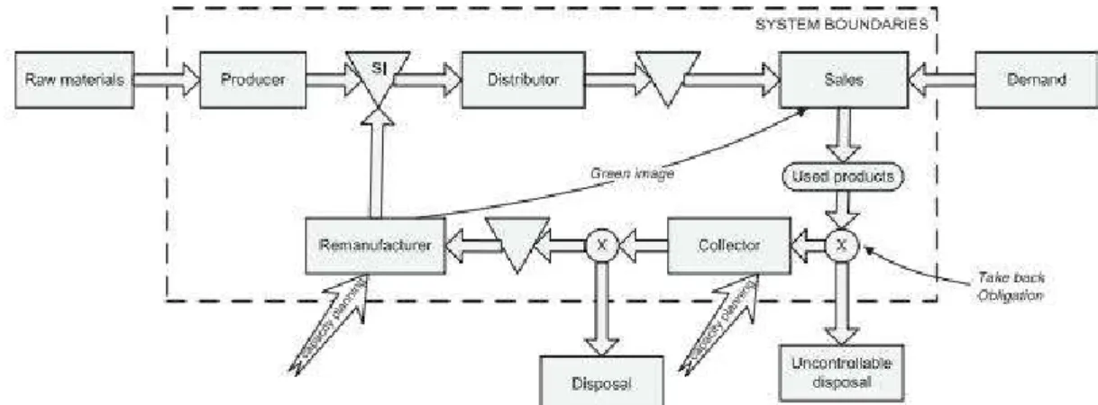
The key parameter for a forward supply chain is the number of echelons from the vendor of raw materials to the end user. Reverse supply chains in comparison, are more complicated as return flows may include products, sub-assemblies and/or materials and can enter the forward supply chain in several return points. Georgiadis (2004) made an interesting presentation of all operations and potential flows in a closed-loop supply chain, which combines forward and reverse supply chains. Specifically, it addresses among others, the collection, inspection/separation, reprocessing (direct reuse, recycling, repair, remanufacturing), disposal and re-distribution of used products as the main operations of a reverse channel. The focus is on a single product closed-loop supply chain which included the following distinct operations: supply, production, distribution, usage, collection (and inspection), remanufacturing and disposal. Figure 1 presents the general structure of the system. The forward supply chain includes two echelons viz. producer and distributor. In the reverse channel, it is assumed that the only reuse activity is remanufacturing.

4 Remanufacturing brings the product back into an “as good as new” condition by carrying out the necessary disassembly, overhaul and replacement operations.

Figure 1: Close loop supply chain for remanufacturing process (Source: Georgidis et al., 2006)

The finished products will be first transferred to the distributor and then sold to meet the demand. The product sales at the end of their life-cycle turn-out into used products, which will either be uncontrollably disposed, or collected for reuse. The collected products after inspection either get rejected and controllably disposed or accepted and transferred for remanufacturing. The loop closes with the remanufacturing operation in two ways. Firstly, through the flows of “as good as new” products to the serviceable inventory (SI in Figure 1). Secondly, by raw materials input, total demand, and legislation acts (take-back obligation) shape the external environment of the system.

Two aspects of research interest in this model are “recollection effort” and “remanufacturing time”, which have not been considered so far by the researchers seriously, as their influence on the system behavior is not directly visible. Both of these parameters have influence on remanufacturing performance with specific reference to sustainability, and hence, there is a need to study the significance of their influence. So, this study makes an attempt to develop and SD model of the entire remanufacturing system so as to study the influence of these two key factors.

5. Model construction

The model developed in this research is for an industry, based in India, which deals with the manufacture and market of quality products for the electronic equipment manufacturing industries, including, soldering related equipment and electrostatic discharge control products having many component parts that can be recycled. The cost figures used on the model are based on the actual figures in the industry. Production capacity of the industry is about 1000 items per week with a cycle time of the product varying from 2 to 3 weeks. The serviceable inventory fluctuation based on past records is between 50 to 200 items and distributors‟ inventory fluctuates between 100 to 300 items. Remanufacturing rate on the average is about 50 items per week. The total cost for the company based on past data on an average is about INR 50,000 (US $ 1000) per week.

Initially the raw material is manufactured based on the production rate and the product will pass to the serviceable inventory. The serviceable inventory is a sum of the re-manufactured items and the new items produced from the raw materials. The serviceable inventory goes to the distributor‟s inventory depending upon the order backlog by the shipment to the distributor. From the distributor inventory the items are sold as per the demand. After a period of time, these become used products and they will be collected

5 depending upon the collection capacity, and most of them will become uncontrollable disposed products. The collected products will be inspected and the failure percentage will be recorded and accordingly, the items will be moved to the reusable product inventory for remanufacturing to take place and the unusable items will be disposed.

These products will be remanufactured based on the remanufacturing rate, according to the remanufacturing capacity. As the remanufacturing process increases, environmental consciousness of the users also increases, which increases the green image of the organization. This is very important in the current competitive market condition and can play an important role in gaining the competitive advantage from the others. The Causal diagram and the Stock & Flow diagram of the model are presented in the Figures 2a and 2b. The equations used in the model are listed in the appendix 1.

6 Raw Materials Production Rate Production Capacity Input Rate transportation time Servicable inventory Sl Discrepancy Desired Servicable Inventory Order qty Expected Distributor's Orders Distributor's Orders Orders Backlog Sl Cover Time Dl Adj Time Shipments to Distributor Sl Adj Time Expected Remanufacturing Rate Shipment time Reuse Ratio Distributor's Inventory Sales Demand Backlog Demand Dl Descrepancy Expected Demand Quality Total Demand Actual Quality Quality perspective index Market Share - + + + - -+ + + -+ + -+ -+ + + + -+ + + + + + + + + -+ + + + -Desired Distributor's Inventory + + Dl Cover Time -Remanufacturing Rate + + Remanufacturing Time -Remanufacturing Capacity RC Adding Rate Delay RC Discreapancy RC Expansion rate Reusable products Controllable Disposal Desired Remanufacturing Capacity Reusable Stock Keeping Time Products Accepted for Reuses Inspection

Time Products RejectedFor Reuse

Failure Percentage Disposed Products Collected Products Collection rate Collection Capacity Uncontrollable Disposal Uncontrollably Disposed Products Used Products Approximate Collection Effort for recollection Targeted PEC Desired Collection Capacity Transformation Rate Productivity Person <Productivity Person> PEC Attrition Time to adjust PEC CC Discrepancy CC Expansion Rate Kc Pc Kr Pr <PEC> CC Adding Rate <Delay> + -+ + + + + -+ -+ -+ -+ + - ₊ -+ + Expected Used Products + + -+ -+ + + + + + -+ -+ + + + + -+ + + + -+ + + B B B B B B R R B R

Figure 2a: Stock and flow diagram of remanufacturing system

7 6. Simulation & analysis

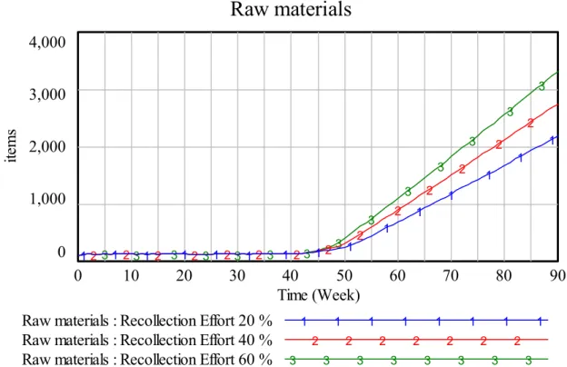
The model was simulated for studying the influence of variation of recollection effort, and remanufacturing time on various endogenous factors of remanufacturing as discussed below. 6.1Influence of recollection effort

Simulation based on recollection effort considers the effort exerted on collecting the used products through advertising, sales promotion, awareness camps, media broadcast etc. The recollection effort was varied from 20% to 60% and after studying the system stabilization for all the factors under consideration, results were plotted for 90 weeks.

6.1.1 Raw materials

It is evident from Figure 3 that initially recollection effort doesn‟t seem to have any influence on recollection of raw material inventory. This is because it takes time for the methods adopted for recollection to be effective, and hence, all the raw material is consumed for the production process till the recollection activity increases and takes its effect, after which, there is a drastic increase in raw material inventory. As the recollection effort increases, there is an increase in raw material inventory.

Raw materials Serviceable inventory Distributors inventory Demand backlog Orders backlog Remanufacturing capacity Reusable products Disposed products Collected products production rate remanufacturing rate RC adding rate controllable disposals products accepted for reuse products rejected for reuse shipment to distributor distributors orders orders backlog reduction rate demand demand backlog reduction rate collection rate Collection capacity CC adding rate Uncontrollably disposed products uncontrolable disposal production capacity

production time _{SI adj time} SI discrepancy desired SI SI cover time expected distributors orders DI DI adj time sales DI discrepancy desired DI DI cover time expected demand D total demand market share delivery time shipment time RC expansion rate RC discrepancy Kr Pr Desired RC RC remanufacturing time RR expected remanufacturing rate reuse ratio expected used products UP used product desired CC CC CC discrepancy Pc CC expansion rate Kc faliure percentage inspection time reusable stock keeping time <reuse ratio> <expected distributors orders> <products accepted for reuse> ordering qty transportation time input rate <demand> Unit time Impulse impulse 2 EC transformation _attrition productivity Targeted EC <desired CC> time to adj EC

quality actual quality quality perspective index effort for recollection app. collection

cost per unit

remanufacturing<remanufacturing_rate> Remanufacturing

Cost

Production cost <production

rate>

Cost of unit item for production Total Cost Raw material cost collection cost <collection rate> Cost of unit item for

raw matwrial

Cost of unit item for collection

<production rate>

Figure 2b: Stock and flow diagram of remanufacturing system

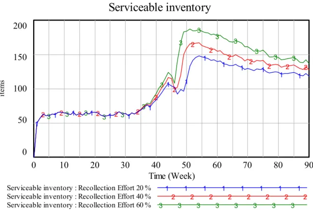
8 6.1.2 Serviceable inventory

It is interesting to observe that it appears as if the effort of recollection has no influence on serviceable inventory for the first about 35 weeks. Moreover, it appears as if, even an increase in the effort of recollection has no influence on serviceable inventory, as all the graphs merge into a single line. There is an increase in serviceable inventory with the distortion type of behavior and the inventory level reaches its peak by about 50th week, after which, it gets stabilized and gradually decreases. The inventory level increases from 120 units to 180 units from 45th to 50th week, when the recollection effort is 60% (Figure 4).

Raw materials

Raw materials : Recollection Effort 20 % 1 1 1 1 1 1 1 1

Raw materials : Recollection Effort 40 % 2 2 2 2 2 2 2

Raw materials : Recollection Effort 60 % 3 3 3 3 3 3 3 3

9

Figure 4: Influence of recollection effort on Serviceable Inventory

6.1.3 Distributors’ inventory

Figure 5: Influence of recollection effort on Distributors‟ Inventory

Distributors‟ inventory peaks to about 290 items in about 45th to 50th week. This is due to the impact of the order backlog on the shipment to distributor, which increases it owing to

Serviceable inventory

Serviceable inventory : Recollection Effort 20 % 1 1 1 1 1 1 1 1

Serviceable inventory : Recollection Effort 40 % 2 2 2 2 2 2 2 2

Serviceable inventory : Recollection Effort 60 % 3 3 3 3 3 3 3 3

Distributors inventory

Distributors inventory : Recollection Effort 20 % 1 1 1 1 1 1 1 1

Distributors inventory : Recollection Effort 40 % 2 2 2 2 2 2 2 2

10 the meeting of the backlog level (Figure 5). Increase in the recollection effort does not seem to have a significant influence on distributors‟ inventory except for the period of quantum rise in the distributors‟ inventory.

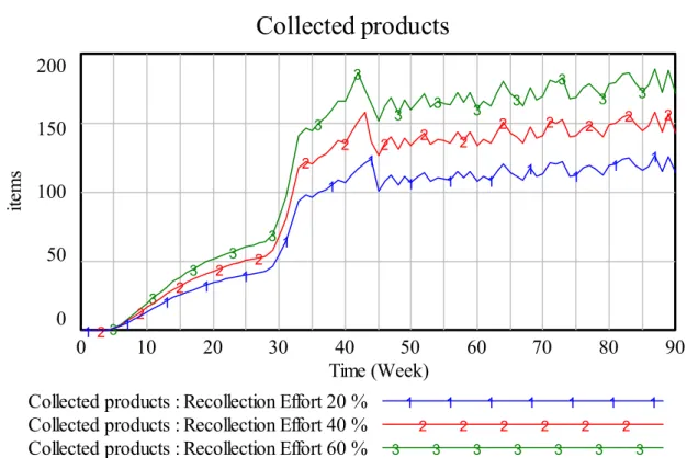
6.1.4 Collected products

Figure 6: Influence of recollection effort on Collected Products

There are two distinct stages of rise in collected products (Figure 6). For the first 30 weeks there will be an exponential increase, and then, from 30th to about 42nd week a quantum rise can be observed. Thereafter, from about 45th week the number of collected products will settle down for an average of about 150 items. However, there is a significant rise (about 100 items when effort is increased from 20% to 60%) in the collected products based on the recollection effort.

6.1.5 Environmental consciousness

The environmental consciousness of people is directly proportional to the recollection effort, obviously (Figure 7). Hence, higher the effort put on recollection, more the environmental consciousness.

Collected products

Collected products : Recollection Effort 20 % 1 1 1 1 1 1 1

Collected products : Recollection Effort 40 % 2 2 2 2 2 2

11 6.1.6 Remanufacturing rate

Figure 8: Influence of recollection effort on Remanufacturing Rate

Initially, remanufacturing rate is nil for about 30 weeks (Figure 8), following which, a drastic increase can be observed up to 45 weeks, and thereafter, the remanufacturing rate

Env Consc

Env Consc : Recollection Effort 60 % 1 1 1 1 1 1 1 1 1

Env Consc : Recollection Effort 40 % 2 2 2 2 2 2 2 2

Env Consc : Recollection Effort 20 % 3 3 3 3 3 3 3 3

remanufacturing rate

remanufacturing rate : Recollection Effort 60 % 1 1 1 1 1 1 1

remanufacturing rate : Recollection Effort 40 % 2 2 2 2 2 2

remanufacturing rate : Recollection Effort 20 % 3 3 3 3 3 3 3 Figure7: Influence of recollection effort on Environmental Consciousness

12 stabilizes. Also, remanufacturing rate increases with increase in recollection effort. This behavior is because of the fact that remanufacturing can be started only after substantial material has been recollected.

6.1.7 Remanufacturing cost .

In the environment of remanufacturing, the total cost/week is given by:

Total Cost = Production cost + Remanufacturing Cost + Raw material cost + Collection cost Remanufacturing cost will be nil until the products are recollected, serviced and introduced to the manufacturing line (the first 30 weeks) (Figure 9a), after which, it suddenly increases during the next 15 weeks and then tries to stabilize. Again, the higher the recollection effort, the higher will be the remanufacturing cost.

The point to be noted is, despite the higher remanufacturing cost for a period of 15 weeks commensurate with the 30th week (Figure 9b), the total cost drastically falls down after the 45th week and stabilizes by the 55th week. One more interesting observation is that up to 40th week higher recollection effort does not guarantee lower total cost, due to the initial operating costs in the system, however, after the 40th week, the more the effort of recollection the lesser will be the total cost. For about 60 items remanufactured, savings of INR. 12,500 (250 US $) per week can be achieved by increasing the recollection effort by about 40%.

Figure 9a: Effort of Recollection on Remanufacturing cost

Remanufacturing Cost

Remanufacturing Cost : Recollection Effort 60 % 1 1 1 1 1 1 1 1

Remanufacturing Cost : Recollection Effort 40 % 2 2 2 2 2 2 2 2

Remanufacturing Cost : Recollection Effort 20 % 3 3 3 3 3 3 3 3

13 Policy implications

 Raw materials: Even though the effort of recollection appears to have no influence in the beginning, after about 45 weeks, higher the effort of recollection greater will be the raw material inventory. So, the firm should not ignore the recollection effort, instead, enhance recollection efforts, as considerable increase (linear growth) in raw material for remanufacture can be expected in the long run.

 Serviceable inventory: A quantum jump is observed after 45 weeks, and thereafter a serviceable inventory of about 120 items can be maintained on an average. Accordingly, the company may plan the production process.

 Distributor inventory: Again, a quantum jump is observed in the 45th week, but the point to be noted is that enhancement of recollection effort has no significant influence on distributor inventory after the quantum increase period. The implication is that the firm can be prepared for a distributor inventory of about 180 to 200 items on an average, after about 70 weeks of operations, but should be prepared to hold stock of about 300 items during the peak period.

 Collected products: Up to the 30th week, the increase of recollected products will be gradual but a quantum rise after 28 weeks may be expected. On an average, 150 items can be collected after 45 weeks of operation and if the maximum recollection effort is aimed by the company, it should be prepared to handle 200 collected products after 40th week.

 Environmental consciousness: It is obvious that higher the effort of recollection greater will be the environmental consciousness, but the awareness increases rapidly at the initial stages and will be gradual at latter stages, say after 50 weeks of operations. It is natural that it is only in the initial stages the company will have to exert more effort to reach the mass for recollecting the used products, but after certain time, people will automatically get tuned to the process and approach the retailers for facilitating recollection.

 Remanufacturing rate: The company will have to prepare itself to be ready by 30 weeks of its operations on recollection effort to remanufacture about 80 items per

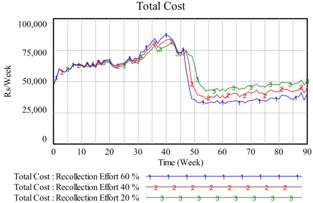
Figure 9b: Influence of recollection effort on Total Cost 100,000 75,000 50,000 25,000 0 3 3 3 3 3 3 3 3 3 3 3 3 3 3 2 2 2 ₂ 2 2 2 2 2 2 2 2 2 2 1 1 1 1 1 1 1 1 1 1 1 1 1 1 0 10 20 30 40 50 60 70 80 90 Time (Week) R s/ W ee k

Total Cost : Recollection Effort 60 % 1 1 1 1 1 1 1 1 1

Total Cost : Recollection Effort 40 % 2 2 2 2 2 2 2 2

14 week if they exert 60% of recollection effort. On an average, it is possible to maintain a constant remanufacturing rate of about 50 items per week after the 45th week, if a moderate recollection effort (about 40%) is exerted.

 Remanufacturing cost: After 30th week as the remanufacturing rate shoots up, correspondingly the total cost of production also shoots up gradually from INR 50,000 (US $ 1,000) per week to about 87,500 (US $ 1,750) per week. The management should not be mislead by this rise in the cost of production, as the remanufacturing concept is aimed towards long term savings in cost as well as ensuring sustainability through environmental protection. This is revealed through the lowering of the cost after 45weeks of operations, where a sudden fall in total cost from about INR 75, 000 (US $ 1,500) to an average of INR 37,500 (US $ 750) in a span of 10 weeks, and thereafter, remaining almost constant for the future operations for a remanufacturing rate of about 60 items per week.

6.2Remanufacturing time

Remanufacturing time is the cycle time for remanufacturing process. As it is an exogenous factor, it is important to study its influence on the entire remanufacturing process. In the industry under consideration, on an average, the remanufacturing time can be varied (through resource manipulation), from 2 to 4 weeks as observed through the past records. 6.2.1 Raw materials

Figure 10: Influence of Remanufacturing Time on Raw Material

It is clear that until the 50th week the consumption of raw materials is not influenced by the remanufacturing time (Figure 10). But after that period, there will be a substantial linear increase. This is due to the reduction in usage rate of raw material due to the increase in the remanufacturing rate.

Raw materials

Raw materials : remanufacturing time 2 1 1 1 1 1 1 1 1

Raw materials : remanufacturing time 3 2 2 2 2 2 2 2 2

15 6.2.2 Serviceable inventory

Figure 11: Influence of Remanufacturing Time on Serviceable Inventory

Serviceable inventory level increases abruptly in the first week itself and it appears as if the increase in cycle time from 2 to 4 weeks has no influence on it (figure 11). However, after the 40th week, the lesser the remanufacturing time, the higher will be the serviceable inventory with a rise from 50th to 55th week, after which, it settles for an average of about 120 items. The point to be observed is that as the remanufacturing time increases, the serviceable inventory level decreases. This is due to the fact that as the remanufacturing time increases, there ought to be reduction in number of remanufactured items coming out of the system. 6.2.3 Distributors inventory

There is a notable increase in level of distributors‟ inventory compared to the serviceable inventory even though both the graphs follow almost identical pattern (Figure 12). Deeper analysis delineates the fact that the order backlog acts on the distributor inventory along with the serviceable inventory, due to which, a sudden rise is recorded. Further, unlike serviceable inventory, in case of distributors‟ inventory, after reaching the threshold value (50th week), the inventory level decreases with the decrease in remanufacturing time. This is an important revelation as far as distributors‟ inventory is concerned and has a direct bearing on the long term perspective of the remanufacturing operations.

Serviceable inventory

Serviceable inventory : remanufacturing time 2 1 1 1 1 1 1 1

Serviceable inventory : remanufacturing time 3 2 2 2 2 2 2

16

6.2.4 Reusable products

Figure 13: Influence of Remanufacturing Time on Reusable Product

It is important to study the fluctuation in the reusable products based on the variation in remanufacturing time. The number of reusable products gets stabilized after the 45th week, as

Distributors inventory

Distributors inventory : remanufacturing time 2 1 1 1 1 1 1 1

Distributors inventory : remanufacturing time 3 2 2 2 2 2 2

Distributors inventory : remanufacturing time 4 3 3 3 3 3 3 3

Reusable products

Reusable products : remanufacturing time 2 1 1 1 1 1 1 1 1

Reusable products : remanufacturing time 3 2 2 2 2 2 2 2

Reusable products : remanufacturing time 4 3 3 3 3 3 3 3

17 it is a function of recollection capacity (Figure 13). Initially, the number of reusable products collapses and records an exponential growth only after 5 weeks of operations and a drastic increase is observed thereafter in two distinct stages. However, after 45th week the number of reusable products settles down to an average of about 100 items. The remanufacturing time variation appears to be passive up to 40th week, after which, it can be observed that there is a significant reduction in the reusable product level with shorter remanufacturing time. An important observation through simulation is that - to maintain an average of reusable products level of at least 100, the remanufacturing time must be set to at least 3 weeks.

6.2.5 Remanufacturing rate

Remanufacturing starts only after 30 weeks after the release of the product to the market and the rate suddenly increases over 50 items/week in a span of about 12 weeks and settles to an average of about 40 items/week (Figure 14). The influence of remanufacturing time is dominant after about 40th week, and obviously, the decrease in remanufacturing time (cycle time) increases the remanufacturing rate.

6.2.6 Remanufacturing cost

Lower the remanufacturing time, higher will be the remanufacturing rate (which is controlled by a threshold value of remanufacturing capacity), and hence, the remanufacturing cost is higher in the long term. Therefore, remanufacturing cost increases with the remanufacturing rate from the 30th week, and settles for about INR 9000 (180 US $) per week (Figure 15a).

remanufacturing rate

remanufacturing rate : remanufacturing time 2 1 1 1 1 1 1 1

remanufacturing rate : remanufacturing time 3 2 2 2 2 2 2 2

remanufacturing rate : remanufacturing time 4 3 3 3 3 3 3 3

18

Figure 15b: Influence of Remanufacturing Time on Total Cost

The Total cost will be the highest for the period of peak remanufacturing rate (40th to 45th week) and settles to a minimum value (about INR 48,000 (US $ 960)) after the 55th week (Figure 15b). It can be observed that that once the remanufacturing starts there will be a

Remanufacturing Cost

Remanufacturing Cost : remanufacturing time 2 1 1 1 1 1 1 1

Remanufacturing Cost : remanufacturing time 3 2 2 2 2 2 2

Remanufacturing Cost : remanufacturing time 4 3 3 3 3 3 3 3

Total Cost

Total Cost : remanufacturing time 2 1 1 1 1 1 1 1 1 1

Total Cost : remanufacturing time 3 2 2 2 2 2 2 2 2

Total Cost : remanufacturing time 4 3 3 3 3 3 3 3 3 3

19 drastic reduction in production cost, which stabilises over a period of time. To minimize the total cost, the plant should operate on minimum possible remanufacturing time (after 50th week).

Policy implications:

 Raw material requirements: Lower the remanufacturing cycle time, higher will the raw material requirements, reason being obvious. However, the simulation results do not show any change in raw material requirements for the first 50 weeks, after which, the above fact is revealed. The reason for this could be that a change in one week cycle time may be too small to cause variations, but over a period of time when the number of recollected products reaches the peak, even a one week shortening of remanufacturing time can cause substantial change in raw material requirements. So, the manufacturing system should prepare itself for higher rates of production well in advance.

 Serviceable Inventory: After the 50th week, lower the remanufacturing time, higher will be the serviceable inventory level, as it is a function of production rate, remanufacturing rate and shipment to distributor. It is very clearly implied that if reducing the remanufacturing time is in the agenda, then higher stock of serviceable inventory may have to be accommodated.

 Distributors’ Inventory: Distributors‟ inventory reduction with lower

remanufacturing time is possible only after 50 weeks of operations. Moreover, for the first 45 weeks, attempts to reduce remanufacturing time will have no bearing on inventory.

 Reusable Product: Increase in the consumption of reusable parts with the increase in remanufacturing time is possible only after about 42 weeks of operations. A steady consumption of about 100 items for about 3 weeks remanufacturing time can be expected only after this period.

 Remanufacturing Rate: Increase in remanufacturing rate is possible only after 30 weeks of operations. A steady remanufacturing rate, of about 35 items per week, can be obtained only after 42 weeks of operations.

 Remanufacturing Cost: It is possible to decrease the total cost with reduced remanufacturing time (2 weeks) after 50 weeks of operations. The plant can be run at a total cost of about INR 48,000 (US $ 960) after about 55 weeks.

7. Validation and testing

Validation of the SD model is basically through testing the model by a set of tools and procedures (Sterman 2000). Following tests have been performed to validate the model: Table 1: Tool and procedures used in validation:

Test Purpose of Test Tools and Procedures used

1. Boundary

Adequacy Are the important concepts for addressing the problem endogenous to the model?

Does the behaviour of the model change

significantly when

Model boundary charts, subsystem diagrams, causal diagrams, stock and flow maps, and direct inspection of model equations have been carried out (Fig.2a & 2b).

When one of the boundary conditions viz. maximum production capacity was increased to 5000 items from 1000 items,

20 boundary assumptions are

relaxed? Do the policy

recommendations change when the model boundary is extended?

the peak inventory value fell down by about 30 items.

Yes, in the above case when the production capacity has been increased, the policy recommendation would be for a reduced number of serviceable inventories. 2. Structure

Assessment

Is the model structure consistent with relevant descriptive knowledge of the system?

Does the model conform to basic physical laws such as conservation laws?

Do the decision rules capture the behaviour of the actors in the system?

Policy structure diagrams, causal diagrams, stock and flow maps are in accordance to the literature and direct inspection of model equations indicate that they follow the rules of production. According to the laws of systems thinking, cause and effect are not closely related in time and space. This behaviour is exhibited in all the simulation results.

Partial model tests of the intended rationality of decision rules conform to the basic physical laws such as, increase in remanufacturing rate results in increase of serviceable inventory.

Effort of recollection having no influence on serviceable inventory in the initial stages of remanufacturing, decline in distribution inventory over a period of time, the stabilization of the number of collected products over a period of time etc. are the indications of the capture of behaviour of the actors of the system 3. Dimensional

Consistency Is each equation dimensionally consistent without the use of

parameters having no real world meaning?

Dimensional analysis has yielded positive results. For example:

Remanufacturing rate (Unit: items/Week) =MIN (Reusable product / remanufacturing time, Remanufacturing capacity)

Unit: MIN(items/week, items/week) = items/week

Therefore, the units on either side of the equations match.

4. Parameter

Assessment Are the parameter values consistent with relevant descriptive and numerical knowledge of the system?

Judgmental methods based on interviews, expert opinion, focus groups, archival materials, and direct experience has indicated that the parameters are consistent. 5. Extreme

Conditions

Does each equation make sense even when its inputs take on extreme values?

Every equation has been tested for extreme values. For instance, when the inventory and labour were set to zero, no production was recorded. It means that, the model is

21 Does the model respond

plausibly when subjected to extreme policies, shocks, and parameters?

capable of not losing its confirmations in the eventuality of using extreme values. Yes, when the model was subjected to large shocks and extreme conditions it has still conformed to basic physical laws without compromising on the quality of the output.

6. Integration Error

Are the results sensitive to the choice of time step or numerical integration method?

The time step in half has been used for testing integration and it works well. For instance, the recollection effort was also checked for intermediate values between 20% and 60%. It was observed that, the model integrity was unaffected.

7. Behaviour Reproduction

Does the model reproduce thebehaviour of interest in the system

(qualitatively and quantitatively)?

Does the model generate the various modes of behaviour observed in the real system?

Under the quantitative analysis, the model indicated that the total cost was insensitive to the increase in recollection effort up to about 45th week, thereafter, higher the recollection effort, lesser was the total cost. About INR. 12,500 (250 US $) per week reduction was brought when Recollection effort was increased by 40% just for about 60 items remanufactured.

Qualitatively speaking, the above observation can also be attributed to the laws of fifth discipline by Peter Senge (2000) which says, Cause and effect are not closely related in time and space.

One can see that, it takes time for the recollection efforts to yield results and not as soon as the system is implemented which is quite realistic phenomenon in nature. The underlying reason is that, the customers take time to be fully aware of the benefits of recycling the product, once this happens, they introduce more and more used products into the remanufacturing process and economies of scale start functioning.

The model outputs fit into the general behaviour of manufacturer, distributor and retailer system. For instance, it was seen that, the decrease in remanufacturing time by 50%, increased the remanufacturing rate by 50% which is a realistic mode of behaviour (Fig. 14).

8. Behaviour

22 of the model are changed

or deleted?

(flattening) is observed. 9. Family

Member

Can the model generate the behaviour observed in other instances of the same system?

The system behaviour is in line with the typical bullwhip effect behaviour of the manufacturer-distributor-wholesaler-retailer system.

10.Surprise

Behaviour Does the model generate previously unobserved or unrecognized behaviour?

Accurate, complete, and dated records of model simulations have been maintained. Likely future behaviour of system was observed and found to be in accordance to the natural behaviour. For instance, under normal circumstances, the reduction in total cost after 36 months of operations may go unnoticed, if not for simulation results.

11.Sensitivity

Analysis Numerical sensitivity: the numerical values of Do the parameters change significantly. . .

Behavioural sensitivity: Do the modes of

behaviour generated by the model change significantly . . .

Policy sensitivity: Do the policy implications change Significantly. . . . . . when assumptions about parameters, boundary, and

aggregation are varied over the plausible range of uncertainty?

Univariate and multivariate sensitivity analysis has been performed on the model and the behavioural changes were proportionate to the change of values up to the threshold limit.

Further, it was observed that policy implementation changed significantly when the boundary conditions were different e.g. the recorded 25% reduction in total cost changed drastically when the number of items produced was changed.

12.System

Improvement Did the modelling process help change the system for the better?

The entire modelling exercise was to find whether remanufacturing is worth the effort and does is ensure sustainability. The result and conclusions are in accordance to the laws of systemic thinking that, behaviour grows worse before it grows better (Peter Senge 2000). The model has responded very positively to this fundamental principle (section 6).

8. Conclusion

Today‟s manufacturing industry has to concurrently meet a wide range of diversified challenges as sustainability is more of focus than mere short term profitability. Model based

23 decision making is the key, as it provides an efficient means to look into the future without spending much on prototyping or consumption of resources in various forms. It is an excellent aid to scenario planning and situational analysis.

In this research, two major outcomes have emerged in the field of remanufacturing with sustainability on the focus, and model based management as the approach. Firstly, the research based on modelling and simulation has very successfully proved that the total cost in the remanufacturing scenario can be very successfully brought down when long term focus is adopted as the strategy. For a firm producing an average of about 60 items per week the cost can be reduced by 25% by the end of the first year of operations, by increasing the recollection effort by about 40%. Secondly, it is clear from the simulation that as the remanufacturing time decreases, remanufacturing rate increases, but the total cost decreases on the long term basis. Thirdly, the environmental consciousness of people continuously increases proportional to the recollection effort.

Hence, it is recommended that an improvement in the remanufacturing process is necessary and effort has to be directed towards reducing the cycle time of the remanufacturing process, to gain the benefits like reduced cost, and also, improvement in the green image by reducing the consumption of fresh raw materials. Applying clean, green and lean manufacturing would be one of the methods to achieve it. A sizable number of researchers in remanufacturing have opined that environmental consciousness is good but comes with an expense associated with it. This general notion is dispelled through this research by demonstrating that on a long term basis, sustainability is surely ensured as the total cost will be reduced drastically. This revelation would surely encourage the manufacturers to consider remanufacturing as an option, whenever possible, so that mother earth may be protected against environmental hazards and at the same time profitability is ensured on long term basis.

References

Boulet J.F. and Ali G. (2009), “Multi-objective optimization in an unreliable failure-prone manufacturing system”, Journal of Quality in Maintenance Engineering, vol. 15 no. 4, pp. 397-411.

Georgiadis P. and Vlachos, 2004, “Decision making in reverse logistics using system dynamics”, Yugoslav Journal of Operations Research, vol. 14, no. 2, , pp. 259-72.

Georgidis P., Vlachos D. and Tagaras G., (2006), “The Impact of Product Lifecycle on Capacity Planning of Closed-Loop Supply Chains with Remanufacturing”, Production and Operations Management, vol. 15, no. 4, p. 514.

Grant and Banomyong (2010), “Design of closed-loop supply chain and product recovery management for fast-moving consumer goods”, Asia Pacific Journal of Marketing and Logistics, vol. 22, no. 2, p. 233, Emerald Group Publishing Limited, 1355-5855, DOI 10.1108/13555851011026971.

Hekkert, M.P., van der Pas, F. and Treffers, D.J. (2001), “Dematerialization and sustainable product service systems”, Sustainable Services and Systems: Transition towards Sustainability? Towards Sustainable Product Design, Proceedings of the 6th International Conference, 29-30 October, The Center for Sustainable Design, Amsterdam, p. 116. Hesselbach J. and Herrmann C. (eds.), (2011), Glocalized Solutions for Sustainability in

Manufacturing: Proceedings of the 18th CIRP International 497 Conference on Life Cycle Engineering, Technische Universität Braunschweig, Braunschweig, Germany, DOI 10.1007/978-3-642-19692-8_86, © Springer-Verlag Berlin Heidelberg.

Jan M. and Noortwijk V., (2000), Journal of Quality in Maintenance Engineering, vol. 6 no. 2, pp. 113-122.

24 Kapetanopoulou P., and Tagaras G., (2009), An empirical investigation of value-added product recovery activities in SMEs using multiple case studies of OEMs and independent remanufacturers, Flex Service Manufacturing Journal), vol. 21, pp. 92–113. King, A.M., Burgess, S.C., Ijomah, W., and Mcmahon, C.A. (2006): Reducing waste: Repair,

recondition, remanufacture or recycle? Sustainable Development vol. 14, no. 4, pp. 257-267.

Mardin and Arai, (2011), “A System Dynamics Model For Replacement and Overhaul Policy for Capital Asset Subject to Technological Change, Conference Proceedings, The 29th

International Conference of the System Dynamics Society

Washington, DC, ISBN 978-1-935056-08-9.

Rogers, D.S. and Tibben-Lembke, R. (2001), „„An examination of reverse logistics practices‟‟, Journal of Business Logistics, Vol. 22 No. 2, pp. 129-48.

Scarf P.A., and Bouamra O. (1999), Journal of Quality in Maintenance Engineering, vol. 5 no. 1, pp. 40-49, © MCB University Press.

Sterman J.D. (Ed.) (2000), Business Dynamics: Systems Thinking and Modeling For a Complex World. Newyork: McGraw-Hill.

Stock, J.R. (1992), “Reverse Logistics Programs”, Council of Logistics Management, Oak Brook, IL.

Stock, J.R. (1998), “Development and Implementation of Reverse Logistics Programs”, Council of Logistics Management, Oak Brook, IL.

Thierry, M., Salomon, M., Van Nunen, J. and Van Wassenhove, L. (1995), „„Strategic issues in product recovery management‟‟, California Management Review, vol. 37, no. 2, pp. 114-35.

Towill D. R., (1996), “Industrial dynamics modelling of supply chains”, Logistics Information Management, vol. 9, issue 4, pp. 43-56.

Warsen J, Laumer M., and Momberg W., (2011), “Comparative Life Cycle Assessment of Remanufacturing and New Manufacturing of a Manual Transmission”, Glocalized Solutions for Sustainability in Manufacturing: Proceedings of the 18th CIRP International Conference on Life Cycle Engineering, Technische Universität Braunschweig, Braunschweig, Germany, Springer-Verlag Berlin Heidelberg.

25 Appendix 1 Actual quality=0.9 Units: Dmnl "App. collection"=0.6 Units: Dmnl Attrition=0.1*transformation Units: people/Week CC=12 Units: Week

CC adding rate=DELAY FIXED (CC expansion rate, 24, 0) Units: items/ (Week*Week)

CC discrepancy=IF THEN ELSE (Impulse>0, desired CC-Collection capacity, 0) Units: items/Week

CC expansion rate=MAX (Kc *CC discrepancy, 0) Units: items/ (Week*Week)

Collected products=INTEG (collection rate-products accepted for reuse-products rejected for reuse, 0)

Units: items

Collection capacity= INTEG (CC adding rate,0) Units: items/Week

Collection cost= Cost of unit item for collection*collection rate Units: Rs/Week

Collection rate= MIN (Collection capacity, used product) + (productivity person*PEC) Units: items/Week

Controllable disposals= Reusable products/reusable stock keeping time Units: items/Week

Cost of unit item for collection=10 Units: Rs/items

Cost of unit item for production=20 Units: Rs/items

Cost of unit item for raw material=75 Units: Rs/items

Cost per unit remanufacturing=25 Units: Rs/items

26 D=12

Units: Week Delivery time=1

Units: Week

Demand=total demand*market share*quality Units: items/Week

Demand backlog= INTEG (demand-demand backlog reduction rate, 0) Units: items

Demand backlog reduction rate=sales Units: items/Week

Desired CC=DELAY1I (used product, CC, used product) Units: items/Week

Desired DI=expected demand*DI cover time Units: items

Desired RC= DELAY1I (products accepted for reuse, RC, products accepted for reuse) Units: items/Week

Desired SI=expected distributors orders*SI cover time Units: items DI=12 Units: Week DI adj time=2 Units: Week DI cover time=1.2 Units: Week

DI discrepancy=MAX (desired DI-Distributors inventory, 0) Units: items

Disposed products= INTEG (controllable disposals + products rejected for reuse, 0) Units: items

Distributors inventory= INTEG (shipment to distributor-sales, 0) Units: items

Distributors orders=expected demand + DI discrepancy/DI adj time Units: items/Week

27 Units: Dmnl

Expected demand=DELAY1I (demand, D, demand) Units: items/Week

Expected distributors orders=DELAY1I (distributors orders, DI, distributors orders) Units: items/Week

Expected remanufacturing rate=DELAY1I (remanufacturing rate, RR, remanufacturing rate) Units: items/Week

Expected used products=DELAY1I (used product, UP, used product) Units: items/Week

Failure percentage=0.2 Units: Dmnl FINAL TIME = 300

Units: Week

The final time for the simulation Impulse=PULSE TRAIN (0, 50, Pc, 300)

Units: Dmnl

Impulse 2=PULSE TRAIN (0, 50, Pr, 300) Units: Dmnl

INITIAL TIME = 0 Units: Week

The initial time for the simulation Input rate=ordering qty/transportation time

Units: items/Week Inspection time=1 Units: Week Kc=1 Units: 1/Week Kr=1 Units: 1/Week

Market share=0.1+0.03*reuse ratio Units: Dmnl

Ordering qty=demand*Unit time Units: items

28 Units: items

Orders backlog reduction rate=shipment to distributor Units: items/Week

Pc=50

Units: Week

PEC= INTEG (transformation-attrition, 100) Units: people

Pr=50

Units: Week Production capacity=1000

Units: items/Week

Production cost=Cost of unit item for production*production rate Units: Rs/Week

Production rate=MAX (MIN (MIN (Raw materials/production time, production capacity), expected distributors orders-expected remanufacturing rate + SI discrepancy/SI adj time), 0)

Units: items/Week Production time=2

Units: Week Productivity person= 2

Units: items/people/Week

Products accepted for reuse=Collected products*(1-faliure percentage)/inspection time Units: items/Week

Products rejected for reuse=Collected products*failure percentage/inspection time Units: items/Week

Quality=actual quality*quality perspective index Units: Dmnl

Quality perspective index=0.8 Units: Dmnl

Raw material cost=production rate*Cost of unit item for raw material Units: Rs/Week

Raw materials= INTEG (input rate-production rate, 100) Units: items

RC=12

29 RC adding rate=DELAY FIXED (RC expansion rate, 24, 0)

Units: items/ (Week*Week)

RC discrepancy=IF THEN ELSE (impulse 2>0, Desired RC-Remanufacturing capacity, 0) Units: items/Week

RC expansion rate=MAX (Kr*RC discrepancy, 0) Units: items/ (Week*Week)

Remanufacturing capacity= INTEG (RC adding rate, 0) Units: items/Week

Remanufacturing Cost= cost per unit remanufacturing*remanufacturing rate Units: Rs/Week

Remanufacturing rate= MIN (Reusable products/remanufacturing time, Remanufacturing capacity)

Units: items/Week Remanufacturing time=2

Units: Week

Reusable products= INTEG (products accepted for reuse-controllable disposals-remanufacturing rate, 200)

Units: items

Reusable stock keeping time= 2 Units: Week

Reuse ratio=ZIDZ (expected remanufacturing rate, expected used products) Units: Dmnl

RR=48

Units: Week

Sales= MIN (Demand backlog, Distributors inventory)/delivery time Units: items/Week

SAVEPER = TIME STEP Units: Week [0,?]

The frequency with which output is stored

Serviceable inventory= INTEG (production rate + remanufacturing rate-shipment to distributor, 0)

Units: items Shipment time=1

Units: Week

30 Units: items/Week SI adj time=2 Units: Week SI cover time= 1.2 Units: Week

SI discrepancy= desired SI-Serviceable inventory Units: items

Targeted PEC= desired CC/productivity person Units: people

TIME STEP = 1

Units: Week [0,?]

The time step for the simulation Time to adj PEC=3

Units: Week

Total Cost= Production cost + Remanufacturing Cost + Raw material cost + collection cost Units: Rs/Week

Total demand=RANDOM UNIFORM (800, 1000, 2) Units: items/Week

Transformation= (Targeted PEC-PEC)/time to adj PEC Units: people/Week

Transportation time= 1 Units: Week

Uncontrollable disposal= used product-collection rate Units: items/Week

Uncontrollably disposed products= INTEG (uncontrollable disposal, 0) Units: items

Unit time=1

Units: Week UP=48

Units: Week

Used product= ("app. collection"+effort for recollection)*sales Units: items/Week