Texture classification of fabric defects using machine learning

ISSN: 2088-8708, DOI: 10.11591/ijece.v10i4.pp4390-4399  4390

Texture classification of fabric defects using machine learning

Yassine Ben Salem, Mohamed Naceur Abdelkrim Engineering School of Gabes, University of Gabes, Tunisia

Article Info ABSTRACT

Article history: Received Nov 25, 2019 Revised Feb 29, 2020 Accepted Mar 9, 2020

In this paper, a novel algorithm for automatic fabric defect classification was proposed, based on the combination of a texture analysis method and a support vector machine SVM. Three texture methods were used and compared, GLCM, LBP, and LPQ. They were combined with SVM’s classifier. The system has been tested using TILDA database. A comparative study of the performance and the running time of the three methods was carried out. The obtained results are interesting and show that LBP is the best method for recognition and classification and it proves that the SVM is a suitable classifier for such problems. We demonstrate that some defects are easier to classify than others.

Keywords: Image processing Machine learning Pattern recognition Texture analysis

Woven fabric defects Copyright © 2020Institute of Advanced Engineering and Science. All rights reserved. Corresponding Author:

Yassine Ben Salem,

National Engineering School of Gabes, University of Gabes,

Road Omer Ibn Elkhattab, Zrig, University of Gabes, Tunisia County 6029, Tunisia, TN. Email: [email protected]

1. INTRODUCTION

In order to maintain the high quality standards established for the clothing industry, Textile manufacturers have to monitor the quality of their products. Therefore, textile quality control is a key factor for the increase of competitiveness of their companies. Textiles faults have traditionally been detected by human visual inspection; skilled worker could at most detect and distinguish 70% of all fabric defects. Then, some defects are classified as reparable because they can be processed through some usual operations by workers and will leave no trace after that. In the other hand, those irreparable defects have a great impact on the quality of cloth which should be eliminated in production and later picked out as many as possible. That’s why we should work on an automaticvisual inspectionand conceive a system to substitute the role of textile workers and surpass their ability in speed and accuracy.

In the past, a lot of work has been done focused on automatic fabric defect detection [1-4]. Fabric defect classification has not yet attracted a wide research interest. Also, it is very rare that we have based on the texture of tissue in the automatic visual inspection visualization despite the appearance of new texture methods in recent years such as Features Extracted from Co-occurrence Matrix GLCM [5-7], or Local Binary pattern LBP [8, 9] or local phase quantization LPQ [10].

The object classification problem is divided into two categories: feature extraction and classification. For the classification, most researchers used the neural network as a classifier, but it is proved that it has shown weak performances and among all, it has a too-long running time [11]. All the research works are based on three approaches: spectral, statistical, and model-based. The statistical approaches, texture features extracted from co-occurrence matrix, mean and standard deviations of sub blocks [12], autocorrelation of images or sub-images [13], and KarhumenLoeve transform have been used for the fabric defects detection [14]. In [15], Bodnarovause the normalized cross-correlation functions for defects detection of textile fabrics. Many model-based techniques for fabric defect detectionwereexisted, for example,

Cohen and al [16] used a Markov random field (MRF) model for defect fabrics inspection. Chen and Jain [17] used a structural approach to detect defects in images based on texture. In [18] they implemented an MRF-based method. Finally, Tajeripourhas used local binary patterns (LBP), this method is known to be a highly discriminative texture operator [19]. In this paper, we build upon previous work to establish a comparative study of three methods based on texture: LBP method, the co-occurrence matrix method, and LPQ method. We choose the SVM classifier to be combined with texture models; it is known to be suitable in this case [20, 21].

2. RESEARCH METHOD

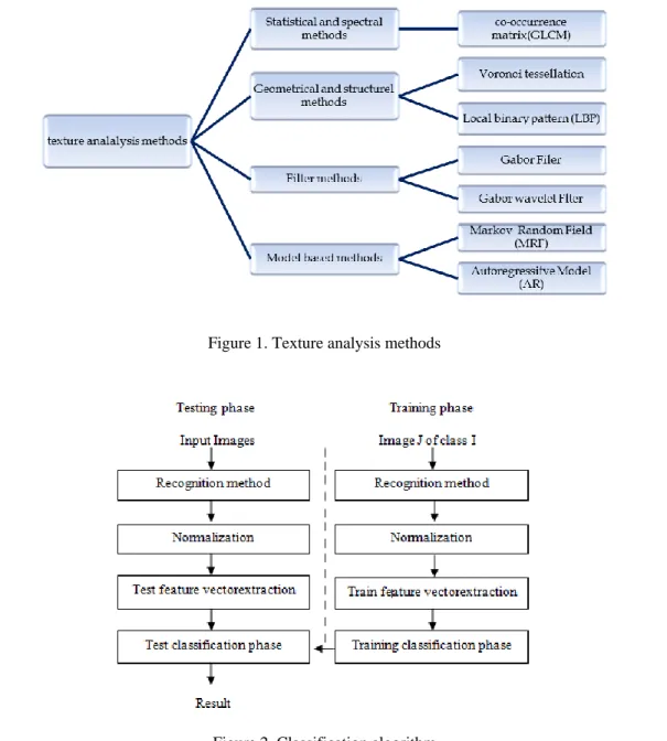
In many applications,especially in industrial surface inspection,texture analysis is an important issue in image processing, medical imaging [5], content-based image retrieval remote sensing [8], and document segmentation, etc. Since the acquisition of images, orientation can be a problem. In the past, some texture analysis methods have not considered this, but recently an increasing amount of attention has been given to invariant texture analysis that’s why many methods for rotation invariance have been proposed. We note many approaches for texture analysis, which can be classified: statistic, structural, model-based and transform-based methods Figure 1. We have elaborated on an algorithm based on the organigram presented in Figure 2. The train and the test feature vectors obtained are implemented in the support vector machine classifier.

Figure 1. Texture analysis methods

2.1. LBP method

TimoOjala has introduced the first LBP operator in 2002, which is evaluated us a robust mean of the texture description of images [22]. In LBP, the pixels are labels by thresholding the 3×3 neighborhood of each pixel with the center value, the result is a binary number. Finally, the histogram of the labels will be enter as a texture descriptor, see Figure 3.

Figure 3. The histogram of the labels

Later, this LBP was extended by using neighbourhoodsfor many sizes [22]. If we usea bi-linearly interpolating and the circular neighbourhoods of the pixel values, we can allow any number of pixels in the neighbourhood and radius. So we obtain a new extensionof the LBP called uniform patterns. The LBP operator is called uniform if it contains at most two transitions (bitwise) from 0 to 1 or vice versa when the binary string is considered circular. A is the histogram of labeled image M(x, y), it can be defined as:

(1)

where n: number of labels produced by the LBP, and I

(2) A is the histogram and represent the distribution of the local micro-patterns of the texture image. (R, P) are the two parameters in this histogram, P is the points (sampling) on a circle radius R see Figure 4. The features vector of the histogramformed will be the input vector for the SVM classification step.

Figure 4. Three circular neighborhoods: ( 1, 6), (1, 8), (2, 16)

2.2. GLCM method

The Gray-Level Co-Occurrence Matrix (GLCM) is the second texture analysis method tested in this work. It based on an extraction of the texture measured from an image. There are three parameters varied in this method: the distance D whereDis the distance between two pixels, the angle θ, it is the angle between two directions, and the offset [22, 23]. For θ, There are four directions: θ = 0°, θ = 45°,θ = 90° and θ = 135° shown in Figure 5. We define the offset parameter:offset= (0 D, -D D,-D 0, -D –D). In our work, we note that we detect a second parameter that affects the result of classification it is the number of gray-levels: the Numlevels. We will demonstrate that this parameter is very influential in the classification results.

Figure 5. GLCM parameters

All the values of GLCM Mmn should benormalized. Than GLCM is expressed by:

(3) The origin of GLCM is the paper [23], Haralick proposed 14 different statistical features in order to estimate the similarity in the texture image. We have tested all the 14 features and we concluded that the most significant ones are 4 features expressed in Table 1, and then we form the GLCM features vector. We consider an image with (N×N) dimension, where m,n formed the coordinates of the GLCM co-occurrence matrix, and Cmn is the corresponding element of (m,n).

Table 1 Haralick’s parameters

Features Formula Contrast

 

 









 

 

The third method is (LPQ) Local Phase Quantization.It is based on localize ofthe phase information extracted using the 2-D DFT or in other way we can say it uses a Fourier transform in a short-term (STFT) computed over M-by-M neighborhoodrectangular. It was used on the blur invariance property of the Fourier phase spectrum [10]. xis the pixel position of the image f(x) defined by:

(4) Which is the basis vector of the 2-D DFT and u is the frequency, and is another vector containing (M×M) image samples from . As it can be noticed from (4), an efficient way of implementing the STFT is to use 2-D convolutions:

for all u. (5)

Computation can be performed using 1-D convolutions for the rows and columns successively since the basic functions are separable, In LPQ only four complex coefficients are considered, corresponding to 2-D frequencies.

(6) a is a scalar frequency below the first zero crossing of that satisfies the condition:

∠G(u) = ∠F(u) for all H(u) ≥0 let

and

(7)

Im{.} andRe{.}return imaginary and real parts of a complex number, respectively. The corresponding 8-by- transformation matrix is:

Then (8)

For each pixel position this results in a vector:

(9) We mark the signs of the real in F(x) and imaginary in F(x) and we record the phase information in the Fourier coefficients by using a simple scalar quantization.

where gj is the j component of the vector: G(x) = [Re{F(x)}, Im{F(x)}]

qj are the integer values between 0 and 255 using LPQ:

(10)

Finally we obtain a feature vector input for the classification phase. 2. 4. Classification phase

We use machine learning and practically the multi-class SVM as a classifier for this study [24]. The main idea of The SVM classifier is to obtain a function f(x) which determines the optimal hyperplane that separe the different classes’ zones. We obtain this hyperplane when it managed to separate two classes, or more, of input data points shown in Figure 6. M represents the distance from the hyperplane to the closest point for both classes of data points. In order to maximize the margin M, we consider and the conditions of the problem will be written:

(11) where:

w: a vector defining the boundary, n: number of input of data of SVM, b: a scalar threshold value.

: input data point,

The optimal hyperplane problem of SVM,f(x):

(12)

Figure 6. Optimal separation hyperplane of SVM

In this case we can note that there are more than two types of multi-class classifiers in this SVM algorithm. The first is called one against all and the other is called one against one. We have compared the performance of the two types. The type one against one needs to construct one classifier for two arbitrary classes, i.e. k(k-1)/2 classifiers all together. For One against all trains k classifiers (k is the number of classes). In that case, the classifier tries to separate the class i from the rest. Then the two-class classifiers evaluate the input data and vote on their classes. In this study, we have worked with a toolbox named ‘simpleSVM’in Matlab [25]. We can conclude that it is a simple and efficient toolbox.

3. DATABASE

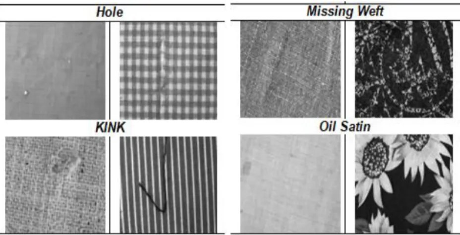
In 1995, the TechnischeUniversitt Hamburgelaborated a database special textile texture images namedTILDA [26], which consists of 8 different classes of woven fabric. The hardest case in this database is that the orientation of the textile is not known. It is an important test of the robustness of our approach. In our study, we have included a new class named “No Defect”. The results show that this class regarded as the best available one. It presents many forms related to the textures analysis and recognition Figure 7.

Figure 7. 4 woven fabric defects class

4. RESULTS AND ANALYSIS

We have chosen to use 5 classes of woven fabric defects, “Hole”, “Kink”, Missing weft”, “oil satin”, and “No defect”; each class contains 100 images: 20 images for training and 80 for the test. In total, we have used 500 samples from the TILDA database see Table 2. The samples are picking randomly.

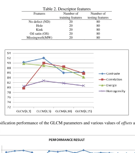
In order to compare the three proposed methods in resolving the problem of classification of woven fabric images, we have started with the GLCM one. In Figure 8, we present the performances of classification using the followingGLCM parameters (contrast, energy, homogeneity, correlation) and varying the offset values. The results of classification presented in Figure 8 shows that the contrast gives a better classification result with 92% compared to other parameters: homogeneity, energy, and correlations. With the GLCM method

we remark that we obtained the best percentage of the successful classified images is 98.25%. It is obtained with the couple (offset,Numlevels)=(6, 3), and the running time is about 44.84 seconds as showed in Figure 9 and Table 3.

Table 2. Descriptor features

Features Number of training features Number of testing features No defect (ND) 20 80 Hole 20 80 Kink 20 80

Oil satin (OS) 20 80

Missingweft(MW) 20 80

Figure 8. Classification performance of the GLCM parameters and various values of offsets and Numlevels

Figure 9. Comparison of classification performance between the three methods

Table 3. Classification performance of the GLCM method

GLCM (level, offset)

Class”OS” Class”MW” Class”Hole” Class”kink” Class”ND” Time (sesond) Result

GLCM(2,3) 95 96.25 83.75 78.75 100 45.35 90.75

GLCM(4,3) 100 95 96.25 90 100 53.36 96.25

GLCM(6,3) 100 98.75 95 97.5 100 44.84 98.25

GLCM(2,5) 98.75 96.25 91.25 36.75 100 69.35 90

GLCM(4,5) 68.75 100 83.75 50 15 69.88 63.5

With the LBP method, we varied two parameters (R, P) and we obtained 99.75 % as the best result percentage illustrated in Table 4. We note that this result is obtained with LBP method and with the couple (1, 16) and in a running time equal to 474.49 seconds. We can conclude that the percentage of this method is higher than the GLCM while the disadvantage it is long run time shown in Figure 10.

Table 4. Classification performance of the LBP method

LBP(R, P) Class”OS” Class”MW” Class”Hole” Class”kink” Class”ND” Time (sesond) Result

LBP(1,4) 93.75 92.5 96.25 95 100 11.69 95.5

LBP(2,4) 78.75 98.75 95 91.25 100 10.7 92.75

LBP(1,8) 100 98.75 91.25 96.25 100 16.18 97.25

LBP(5,8) 67.5 100 90 81.25 100 15.7 87.75

LBP(1,16) 99.75 100 100 98.75 100 474.49 99.75

Figure 10. Comparison of running time of the three methods

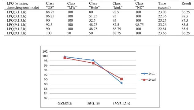
With the LPQ method, we obtain us a result with the combination of the four parameters (win_size, decor, freqstem, and mode)=(3,1,2,h) and the result is about 90.5% shown in Table 5. This method seems to be less accurate than the two other methods. The detailed percentage of correctly classifications for each method is illustrated in Figure 7. We notice that the images with no defects ‘ND’ are easier to classify than the others. Furthermore, the method LBP provides a good classification that reached 98.75% with a short time 16.18s. We can say that the GLCM method can give a good classification rate but with a longer time.

The LPQ method is characterized by its short running time and its classification rate lower than the other techniques precisely of the "Hole" class. Another important result concerning the SVM classifier algorithm is determined; more detailed results are presented in Figure 11. The approach "1vs1" increases the classification rate more than the “1vsall”. For example, the LBP method with parameters (1, 16) leads to 99.75%, whereas with the approach “1vsall” we obtained 99.25 %.

Table 5. Classification performance of the LPQ method

LPQ (winsize, decor,freqstem,mode)

Class

”OS” Class ”MW” Class ”Hole” Class ”kink” Class ”ND” Time (sesond)

Result LPQ(3,1,1,h) 88.75 100 80 92.5 100 23.03 86.25 LPQ(3,1,2,h) 96.25 100 51.25 95 100 22.36 88.5 LPQ(3,1,3,h) 90 100 52.5 95 100 23.25 87.5 LPQ(9,1,1,h) 92.5 100 48.75 87.5 98.75 23.26 85.5 LPQ(9,1,2,h) 90 100 48.75 88.75 100 22.81 85.5 LPQ(9,1,3,h) 100 50 50 88.75 100 23.66 86.25

5. CONCLUSION

We have studied the problem of automatic classification of the woven fabric defects based on texture of the images. The presented work consists on a comparative study of three different approaches: GLCM, LBP and LPQ. Using the GLCM method, after studying the different statistical features, we conclude that only 4 are the most significant Contrast, Homogeneity, correlation, and energy. The best one is the contrast. With this method, we remark that the best performance result ofclassification is about of 98.25% with a 44.84 seconds running time. With the LBP method, based on the property of local image textures and their occurrence histogram, we obtained 97.25 % as the best result percentage with a running time about 16.18 seconds only.

The third method LPQ is based on local frequency coefficient; it showed not bad results with 88.5% performance and 22.36 seconds. The established study proves that SVM is a suitable classifier for such problems. A TILDA database is used to test our algorithm. Some defects which are easier to classify than others, for example, unrelated corpus, hole, and oil satin are easier to classify. In conclusion, we remark that LBP method is the best method for this problem of recognition and classification woven defects, it is characterized also by good running time

REFERENCES

[1] Kumar, Ajay, “Computer-vision-based fabric defect detection: A survey,” IEEE Trans. Ind. Electron, vol. 55, no. 1, pp. 348-363, 2008.

[2] Xie, Xianghua, “A review of recent advances in surface defect detection using texture analysis techniques,” ELCVIA: Electronic letters on computer vision and image analysis, vol. 7, no. 3, pp. 1-22, 2008.

[3] Murino V., Bicego M. and Rossi I. A, “Statistical classification of raw textile defects,” Proceedings of ICIP’O4, vol. 4, pp. 311-314, 2004.

[4] Tsai I. S., Lin C. H., and Lin J.-J, “Applying an artificial neural network to pattern recognition in fabric defects,” Textile Research Journal, vol. 65, no. 3, pp. 123-130, 1995.

[5] Yahia S., Ben Salem Y., and Abdelkrim M. N., “Multiple sclerosis lesions detection from noisy magnetic resonance brain images tissue,” 15th International Multi-Conference on Systems, Signals and Devices, pp. 240-245, 2018.

[6] Yahia S., Ben Salem Y., and Abdelkrim M. N., “Analysis of 3D textures based on features extraction ”. 15th International Multi-Conference on Systems, Signals and Devices, 2018.

[7] Nanni L., Lumini A., Brahnam S., “Survey on LBP based texture descriptors for image processing,” Expert Systemswith Applications, vol. 39, no. 3, pp. 3634-3641, 2012.

[8] Chairet R., Ben Salem Y., and Aoun M., “Features extraction and land cover classification using Sentinel 2 data,” 19th International Conference on Sciences and Techniques of Automatic Control and Computer Engineering, pp. 497-500, 2019.

[9] Ben Salem Y., and Salem Nasri, “Woven fabric defects detection based on texture classification algorithm,” 8th International Multi-Conference on Systems, Signals and Devices, 2011.

[10] Ojansivu V., and Heikkila J., “Blur insensitive texture classification using local phase quantization,” International conference on image and signal, pp. 236-243, 2008.

[11] Ben Salem Y., Nasri S., and TourkiR., “Classification of tissues by neural network,” Proceedings of the IEEE International Conference on Electronics, Circuits, and Systems, 2005.

[12] Zhang X. F. and Bresee R. R., “Fabric defect detection and Classification using image analysis,” Textile Research Journal, vol. 65, no. 1, pp. 1-9, 1995.

[13] Wood E. J., “Applying fourier and associated transforms to pattern characterization in textiles,” Textile Research Journal, vol. 60, no. 4, pp. 212-220, 1990.

[14] Unser M. and Ade F., “Feature extraction and decision procedure for automated inspection of textured materials,” Pattern Recognition Letters, vol. 2, no. 2, pp. 181-191, 1984.

[15] Bodnarova A., Bennamoun M., and Kubik K. K., “Defect detection in textile materials based on aspects of the HVS,” Proceedings of IEEE International Conference on Systems, Man and Cybernetics, vol. 5, pp. 4423-4428, 1998. [16] Cohen F. S., Fan Z., and Attali S., “Automated inspection of textile fabrics using textural models,”

IEEE Transactions on Pattern Analysis and Machine Intelligence, vol. 13, no. 8, pp.803-808, 1991.

[17] Chen J. and Jain A. K., “A structural approach to identify defects in textured images,” Proceedings of IEEE International Conference on Systems, Man, and Cybernetics, vol. 1, pp. 29-32, 1988.

[18] Atalay A., “Automated defect inspection of textile fabrics using machine vision techniques,” M.S. thesis, Bogazici University, 1995.

[19] Tajeripour F., Kabir E., and Sheikhi A., “Fabric defect detection using modified local binary patterns,” EURASIP Journal on Advances in Signal Processing, vol. 2008, pp. 1-12, 2007.

[20] Burges, C. J. C., “A tutorial on support vector machines for pattern recognition,” Data Mining and Knowledge Discovery, vol. 2, no. 2, pp. 121-167, 1998.

[21] Ben Salem Y., and Nasri S., “A comparative study of rotation-invariant texture classification using SVM,” 3rd International Conference on Signals, Circuits and Systems, 2009.

[22] Ojala, T., Pietikäinen, M., and Mäenpää, T., “Multiresolution gray-scale and rotation invariant texture classification with local binary patterns,” IEEE Transactions on Pattern Analysis and Machine Intelligence, vol. 24, no. 7, pp. 971-986, 2002.

[23] Haralick, R. M., Shanmugam, and K., Dinstein, I., “Textural features for image classification,” IEEE Transactions on systems, man, and cybernetics, vol. 3, no. 6, pp. 610-621, 1973.

[24] Wang Z., Xue X., “Support Vector MachinesApplications,” Springer, 2014.

[25] Gaëlle, L., Canu, S., Vishwanathan S.V.N., Alexander, S. J., and Chattopadhyay, M., “Boîte à outils SVM simple et rapide,” Revue d'intelligence artificielle, vol. 19, no. 4-5, pp. 741-767, 2005.

[26] Workgroup on Texture Analysis of DFG, TILDA textile texture database, 1996 http://lmb.informatik.uni-freiburg.de/research/dfg-texture/tilda

BIOGRAPHIES OF AUTHORS

Yassine ben Salem was born in Gabes (Tunisia) on 1973. He began teaching at Tunisia

University in 1999 in the « Higher Institute of Technological Studies of Sousse-ISETSo». He received the State Doctorate in 2011 at the University of Sfax. Since 2013 he has been an Associate Professor in computer science at the “National School of Engineers of Gabes –ENIG”, University of Gabes, He is the member of the Research Laboratory « Modeling, Analysis and Control Systems-MACS-LR16ES22 (www.macs.tn). He has directed more than 50 Engineering projects and master and 3 theses.

Mohamed Naceur Abdelkrim was born in Gabes (Tunisia) on 1958. He began teaching at

Tunisia University in 1981 in the « National School of Engineers of Tunis – ENIT». He received the State Doctorate in 2003. Since 2003 he has been a Professor in Automatic Control at the “National School of Engineers of Gabes –ENIG”, University of Gabes. He is the Head of the Research Laboratory « Modeling, Analysis and Control Systems-MACS-LR16ES22 (www.macs.tn) with about 100 researchers. He has more than 50 publications and more than 200 communications. He has directed more than 50 Thesis