Copyright by
Priyanka Khante 2017
The Thesis committee for Priyanka Khante Certifies that this is the approved version of the following thesis:
Learning Attributes of Real-world Objects by
Clustering Multimodal Sensory Data
APPROVED BY
SUPERVISING COMMITTEE:
Peter Stone, Supervisor Andrea Thomaz
Learning Attributes of Real-world Objects by
Clustering Multimodal Sensory Data
by
Priyanka Khante, B.S.
THESIS
Presented to the Faculty of the Graduate School of The University of Texas at Austin
in Partial Fulfillment of the Requirements
for the Degree of
MASTER OF SCIENCE IN COMPUTER SCIENCE
THE UNIVERSITY OF TEXAS AT AUSTIN May 2017
Acknowledgments
I would like to thank my supervisor, Dr. Peter Stone for his support and advice throughout my Master’s degree. I am also very appreciative of Dr. Andrea Thomaz for so graciously agreeing to be my second reader. I would also like to thank Jivko Sinapov for being my mentor and for his guidance and advice throughout my Master’s thesis. Thank you for being there every step of the way.
I would like to thank my parents and brother for their unwavering support as I continue to pursue higher studies away from home. I also very grateful for the many friends that I have made here, who are always there for me and have helped make Austin a second home.
I would like to thank Maxwell Svetlik for helping me with the data collection process, for spending hours brainstorming all ideas and also for our delightful conversations. Thank you to Arnimal Kaul for always being there and for your patience in the initial stages of my thesis. Thanks for putting up with my ramblings of every detail of every algorithm that I came up with to solve my thesis problem. Thank you, Pranjal Natu, for the little needed distractions and conversations that always helped me relax in times of stress. I would like to thank all the participants of my user study as it would not have been possible to successfully finish my thesis without their time and
effort. I appreciate all your feedback and advice and would definitely use it in the future works. You all made my first user study very enjoyable.
Finally, I am also very appreciative of all my labmates that I have worked with, the times that we have spent together and all the fun that we have had. It is a continuing pleasure to have known and worked with you all. My graduate years would not have been the same without all of you. Thank you for have made these years a very enriching experience.
Learning Attributes of Real-world Objects by
Clustering Multimodal Sensory Data
Priyanka Khante, M.S.C.S
The University of Texas at Austin, 2017
Supervisor: Peter Stone
The goal of this work is to propose a framework for learning attributes of real-world objects via a clustering-based approach that aims to reduce the amount of human effort required in the form of labels for object categorization. Due to clustering, with just a single annotation, we can get information about all the objects in a cluster. In the field of robotics, even though studies have focused on the problem of object categorization, the aspect of the amount of workload for a user has not been explored much. However, as the presence of robots has started growing in our daily lives, it is important to reduce the human effort required in labelling for a robot to learn about its environment. Therefore, we propose a hierarchical clustering-based model that can learn the attributes of objects without any prior knowledge about them. It clusters multi-modal sensory data obtained by exploring real-world objects in an un-supervised fashion and then obtains labels for these clusters with the help of a human and uses this information to predict attributes of novel objects.
Table of Contents
Acknowledgments iv Abstract vi List of Tables ix List of Figures x Chapter 1. Introduction 1Chapter 2. Related Works 4
2.1 Psychology and Cognitive Science . . . 4
2.2 Robotics and Computer Vision . . . 5
Chapter 3. Experimental Methodology 7 3.1 Robot . . . 7
3.2 Exploratory Behaviors . . . 10
3.3 Sensory Modalities . . . 11
3.3.1 Visual Feature Extraction . . . 11
3.3.2 Auditory Feature Extraction . . . 12
3.3.3 Haptic Feature Extraction . . . 12
3.3.4 Proprioceptive Feature Extraction . . . 12
3.4 Sensorimotor Contexts . . . 13
Chapter 4. Theoretical Model 14 4.1 Problem Formulation . . . 14
4.2 Weka and Spectral Clustering . . . 15
4.3 Learning Attributes of Objects . . . 16
4.4.1 Interaction stage . . . 17 4.4.2 Clustering stage . . . 18 4.4.3 Experiment 1: Incremental Learning of Object Attributes 18 4.4.4 Experiment 2: Clustering-based Incremental Learning of
Object Attributes . . . 20 4.4.4.1 Experiment 2a: Labels from an Expert in
Simu-lation . . . 21 4.4.4.2 Experiment 2b: User study with Volunteers . . 28
Chapter 5. Results and Analysis 31
Chapter 6. Conclusion and Future Works 40
Appendix 43
Appendix 1. Result’s Appendix 44
1.1 Training Objects VS Questions Answered Graphs . . . 45 1.2 Kappa Co-efficient VS Questions Answered Graphs . . . 47 1.3 Context and Attribute Mapping Experiment Graphs . . . 49
Bibliography 51
List of Tables
3.1 Attribute Ground Truth Table for all the objects in the dataset 9 3.2 Attribute range cutoffs . . . 9 3.3 Number of features extracted from a particular context for the
different sensor modalities. . . 13 4.1 Context and Attribute Mappings from the prior experiment to
be used for Experiment 2a . . . 24 4.2 Context and Attribute Mapping for Experiment 2b . . . 30 5.1 Variations in labels obtained per attribute from Experiment 2b
with the different users against expert labels used for Experi-ment 2a. . . 35
List of Figures
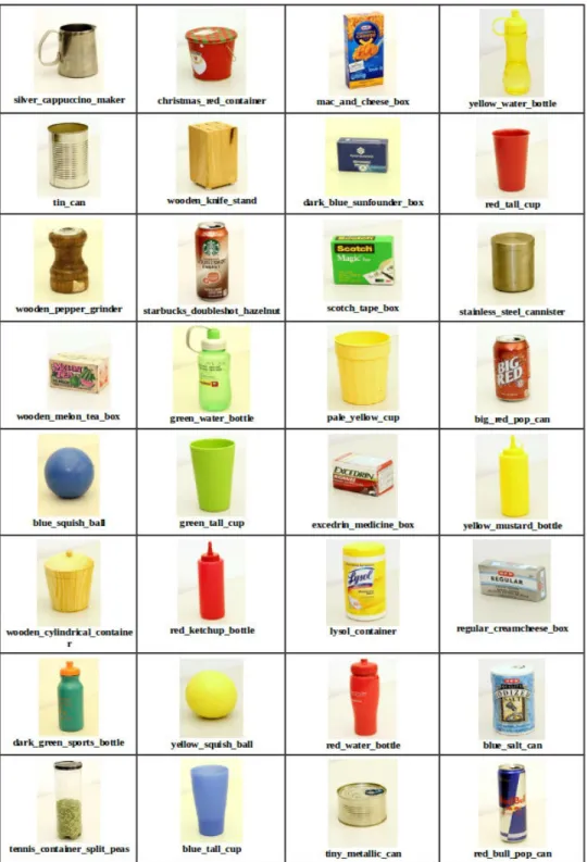
3.1 32 real-world objects used as our data set. . . 8 3.2 10 exploratory behaviors used in our framework. . . 11 4.1 The results of the prior experiment carried out to map which
contexts are best to learn a particular attribute for Experiment 2a. . . 27 4.2 Snapshot of the interface used for our user study. User can
either label, mark a maximum of two outliers or skip a cluster in each iteration. The category of the attribute label is specified on the top. . . 29 5.1 Graphs depicting the kappa coefficient for each question
an-swered by the expert for a particular context to learn a partic-ular attribute. . . 37 5.2 Graphs depicting the rate of number of training objects labelled
per question count for a particular context to learn a particular attribute. . . 39 1.1 The graphs of the all the other contexts for Experiment 1 and
Experiment 2a. The plots showcase the rate of number of train-ing objects labelled per question count for a particular context to learn a particular attribute. The error bars give one stan-dard deviation of uncertainty. It can be seen that Experiment 2a performs better than the baseline of Experiment 1 in terms of number of questions answered. . . 46 1.2 The graphs of the all the other contexts for Experiment 1 and
Experiment 2a. The plots showcase the kappa coefficient for each question answered by the expert for a particular context to learn a particular attribute. The error bars give one standard deviation of uncertainty. It can be seen that Experiment 2a performs better than the baseline of Experiment 1 in terms of number of questions answered. . . 48
1.3 The graphs of the all the other contexts for the prior experi-ment which was done to choose which contexts performed best for a particular attribute. The plots showcase the kappa co-efficient for each question answered and also the total number of questions answered for each attribute. It can be seen that these contexts did not perform well for any of the attributes and hence were not chosen. . . 50
Chapter 1
Introduction
Various studies in psychology have focused on the human skill of cate-gorizing objects. Humans seem to learn this skill at a very young age [3] and it is an important part of their mental development [5]. Various branches of research have shown the importance of object exploration for object catego-rization [9][26]. Most of these works have focused on categorizing objects using only the visual domain [20][22][18] or using toy objects [23]. [7][21] show that an only vision approach is not the best source to learn about object attributes. Other sensory modalities such as auditory, haptic and proprioceptive are also useful in distinguishing between several objects based on their attributes [31] and hence we choose to use a multi-modal approach that combines sensory data from visual, auditory, haptic and proprioceptive domains and use it to learn attributes of 32 real-world objects.
As robots are getting more ubiquitous, object exploration and learning about the environment is of much interest to the robotics community. How-ever, although a robot placed in an unknown environment can go around and explore objects and collect multi-modal sensory data, a human user is still required to connect the data to natural language. Early works concerned with
object labelling and categorization using the multi-modal approach incremen-tally learn the object labels, one at a time, and hence each attribute of the object has to be labelled individually [31][32][11]. This is a major impediment when it comes to large sets of objects where it’s time consuming to label each object individually and small training data can lead to bad performance. A few groups in the computer vision field have explored active learning [14][15][17] and group-based learning [6][19] as solutions to reducing the amount of work-load required from the human for labelling; however they have employed only a vision-based approach (see Chapter 2 for more details).
To address this gap, we propose a framework that grounds the at-tributes of the objects to the robot’s exploratory interactions with the objects. In the first stage, following an unsupervised learning method, the robot first clusters the data from each sensory modality separately which was obtained via performing each of the exploratory behaviors on the objects. Then, the robot obtains labels for these clusters from a human user, thereby reducing the amount of human effort required to label each attribute of an object individu-ally. More specifically, the robot is trying to ground each attribute it learns of an object using the sensory data collected while performing a particular action. In the end, the robot uses this grounded knowledge to predict the attributes of new objects it has not encountered before. We assume that the robot has no prior knowledge about which action is best for learning a particular attribute and hence chooses to cluster and label all sensory data obtained during every behavior and then, in the end, based on the results, deduces which one would
be a best fit to learn a particular attribute.
The model proposed above is explained in greater detail in the follow-ing sections. Chapter 2 discusses some of the prior work that has been done and the inspiration for our methodology from the fields of robotics, computer vision, psychology and cognitive science. Chapter 3 and 4 will cover our ex-perimental methodology in greater detail. Chapter 3 discusses the robot used for our experiment, the real-world objects used along with the attributes that are to be learnt, the exploratory behaviors performed on those objects and the sensory data that was collected. Chapter 4 explains the baseline experiment implemented for our comparison and our clustering approach. Chapter 5 gives the analysis of the results obtained and Chapter 6 concludes this thesis and highlights some of the major takeaways and some future improvements.
Chapter 2
Related Works
Our work focuses on reducing the amount of human effort required in obtaining labels about attributes of objects. Research carried out in the field of psychology and cognitive science shows that children, since a very young age, take advantage of similar characteristics in objects to group them together in order to remember them. We incorporate this clustering based approach in our labelling process, so that we can obtain labels for groups instead of single objects. From, the field of robotics and computer vision, we build upon the idea of active learning of iteratively getting labelled data and group-based learning where human help is required to pick out noisy data.
2.1
Psychology and Cognitive Science
The ability to categorize objects based on their similarities and dis-similarities emerges in children at a very young age. Studies have shown that 4-to-6 year old children employed spontaneous clustering memory strategies to remember objects. They found that the recall rate was much better when the children first sorted the items based on conceptual or perceptual similarities and then stored them in their memory [33]. Younger children tend to group
objects based on color and form first and then at older stages move on to grouping based on conceptual attributes [24]. They also found that 2-year-old children guessed the categories correctly when the objects belonging to same conceptual categories were placed together and they could also figure out the odd one out [10].
The general experiment conducted for these tests are that infants are familiarized with different pairs of objects belonging to the same categories (exploration stage) and then in the testing phase are introduced and are al-lowed to explore novel objects and are asked to pick the objects belonging to the same category [25]. We implemented this same learning methodology in our clustering-based approach where the robot first clustered the sensory data in an unsupervised fashion that it obtained and then got labels for those clus-ters from the human user and this knowledge was tested out on novel objects in the testing phase.
2.2
Robotics and Computer Vision
Reducing the amount of human effort required in labelling for classifica-tion is a rising problem that is being tackled by active learning [14][15][17] and group-based learning [6][19] in the fields of computer vision as large amounts of training data is required for image classification tasks. However, in the field of robotics, this aspect has not received a lot of attention majorly because object categorization for robots has not been explored much for large data sets [23][31][11].
Active learning selects a meaningful subset of the available training data and uses it to train a classifier. However, such a system is only efficient if there exists a subset that is good enough to train the classifiers [37]. Also [36] mentions that active learning usually requires apriori information about the visual concepts in order pick a good subset of the unlabelled data for labelling and also requires prior knowledge on the number of classes present [15]. So, active learning usually starts out with a certain amount of labelled data [28][35][13][34] and then accordingly picks unlabelled data to better the performance of its classifiers. On the other hand, group-based learning assigns labels to a group of training samples. It is more efficient than active learning but it does require more human effort and latency to remove the noisy data if they differ from the dominating class labels [8] or exactly picking those groups that represent a coherent label [36].
However, both of these methods are only concerned with the visual domain and also each of them has it’s own disadvantages. Therefore, we introduce a new clustering based-algorithm that builds on the goodness of both active and group-based learning. Like active learning, it learns iteratively but does not require apriori information regarding the number of classes or concepts. Like group-based learning it picks clusters and provides labels to entire groups but does take human help to pick out the noisy data from the clusters that do not adhere to the dominant label. Moreover, to our knowledge, ours is the first algorithm that does this with multi-modal data in the field of robotics.
Chapter 3
Experimental Methodology
3.1
Robot
The robot used in our experiment is a custom-built two-wheeled robot that uses Segway Robotic Mobility Platform (RMP). There is a 6-DOF Kinova Mico Arm with a two-fingered under-actuated gripper installed on the robot which is used for manipulation purposes. We further equipped the robot with a Asus XTION Pro USB 3.0 RGB and Depth Sensor to capture the visual data and also a Audio-Technica U853AW cardioid microphone used to collect the auditory feedback.
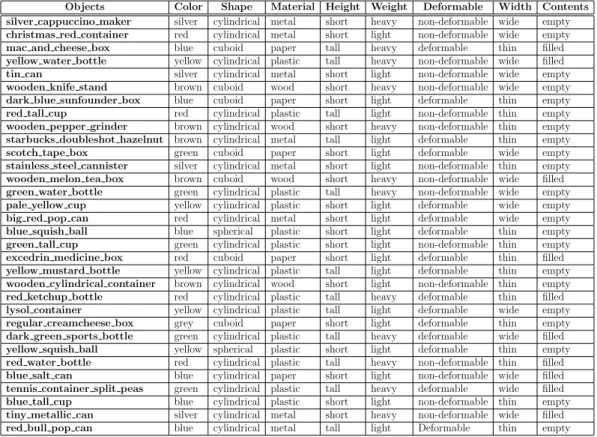
To test out our proposed framework, the robot explored a set of 32 real-world objects. The set mostly consisted of bottles, cans, balls, boxes as shown in Figure 3.1. The objects were chosen in such a way that they varied incolor, shape, material, size (width), height, weight, deformability and contents. The ground truth table for all the objects is shown in Table 3.1 and the attribute categories and ranges are shown in Table 3.2. The height and width of the objects was measured in millimeters and the weight was measured in grams. Some of the objects were filled with water, coffee beans, or lentils so as to make them differ in the attributes learnt.
Objects Color Shape Material Height Weight Deformable Width Contents silver cappuccino maker silver cylindrical metal short heavy non-deformable wide empty
christmas red container red cylindrical metal short light non-deformable wide empty
mac and cheese box blue cuboid paper tall heavy deformable thin filled
yellow water bottle yellow cylindrical plastic tall heavy non-deformable wide filled
tin can silver cylindrical metal short light non-deformable wide empty
wooden knife stand brown cuboid wood short heavy non-deformable wide empty
dark blue sunfounder box blue cuboid paper short light deformable thin empty
red tall cup red cylindrical plastic tall light non-deformable thin empty
wooden pepper grinder brown cylindrical wood short heavy non-deformable thin empty
starbucks doubleshot hazelnut brown cylindrical metal tall light deformable thin empty
scotch tape box green cuboid paper short light deformable wide empty
stainless steel cannister silver cylindrical metal short light non-deformable thin empty
wooden melon tea box brown cuboid wood short heavy non-deformable wide filled
green water bottle green cylindrical plastic tall heavy non-deformable wide empty
pale yellow cup yellow cylindrical plastic short light deformable wide empty
big red pop can red cylindrical metal short light deformable wide empty
blue squish ball blue spherical plastic short light deformable thin empty
green tall cup green cylindrical plastic short light non-deformable thin empty
excedrin medicine box red cuboid paper short light deformable thin filled
yellow mustard bottle yellow cylindrical plastic tall light deformable thin empty
wooden cylindrical container brown cylindrical wood short light non-deformable thin empty
red ketchup bottle red cylindrical plastic tall heavy deformable thin filled
lysol container yellow cylindrical plastic tall light deformable wide empty
regular creamcheese box grey cuboid paper short light deformable thin empty
dark green sports bottle green cylindrical plastic tall heavy deformable wide filled
yellow squish ball yellow spherical plastic short light deformable thin empty
red water bottle red cylindrical plastic tall heavy non-deformable thin filled
blue salt can blue cylindrical paper short light non-deformable wide filled
tennis container split peas green cylindrical plastic tall heavy deformable wide filled
blue tall cup blue cylindrical plastic short light non-deformable thin empty
tiny metallic can silver cylindrical metal short heavy non-deformable wide filled
red bull pop can blue cylindrical metal tall light Deformable thin empty
Table 3.1: Attribute Ground Truth Table for all the objects in the dataset
Short Tall Height (mm) <= 150 >150 Thin Wide Width (mm) <= 61 >61 Light Heavy Weight (g) <= 90 >90
3.2
Exploratory Behaviors
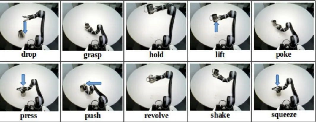
The robot explored the set of 32 objects using 11 exploratory be-haviours. These 10 actions - look, drop, grasp, hold, lift, poke, press, push, revolve, shake and squeeze were done in a sequence, one after the other. Each one of them is shown in Figure 3.2. These behaviors were chosen so that the robot could obtain a grounded object representation irrespective of a particu-lar action and even though its possible that some behaviors are not good for learning any of the attributes, the robot did not have this information apriori. All the behaviors except for thelook behavior were programmed as joint-space trajectories for fixed object positions on a table and executed using the Kinova arm, while thelook behavior consisted of taking 6 RGB-D snapshots of the ob-jects from different viewpoints using the XTION RGB and Depth Sensor. All of the 11 behaviors were performed 6 times on each object, finishing one round on all 32 objects first and then starting the next round in order to minimize any transient noise. So, there were a total of 2112 interactions categorized into 60 trials for each object. The whole data collection process took 12 hours in total.
Figure 3.2: 10 exploratory behaviors used in our framework.
3.3
Sensory Modalities
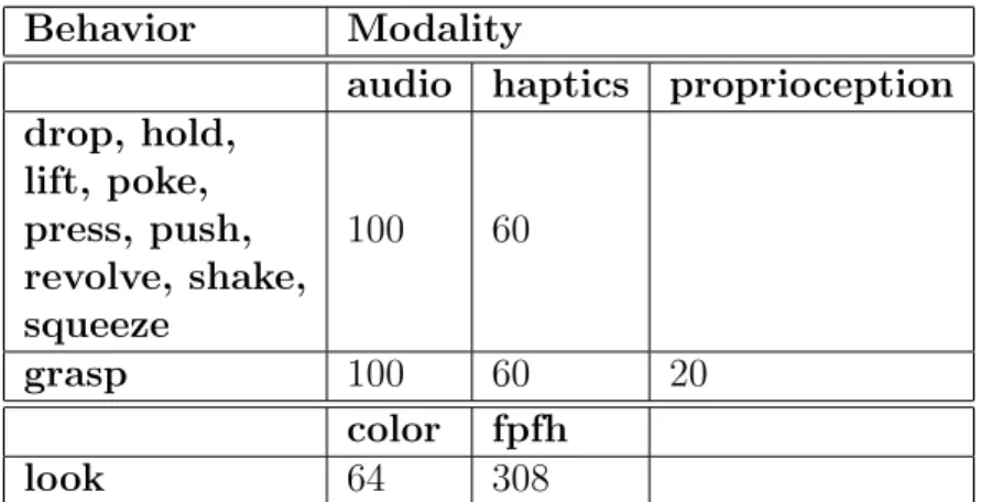
The robot explored the object set using an approach formerly imple-mented in [30]. Table 3.3 gives a short summary of the number of features extracted for each modality and behavior and a detailed description is provided below.
3.3.1 Visual Feature Extraction
During each trial of the look behavior, using the segmented point clouds of the object perceived by the robot, a 8×8×8 RGB color histogram was extracted by binning over each channel. Due to its high-dimensionality, it was further binned into so that the color histogram for each trial was represented by a feature vector of size 64. The binning was done by setting the value of each bin to the average of the values of the color histogram that fell into that bin. Also, Fast Point Feature Histogram (fpfh)[27] from the Point Cloud
Library [2] were used to compute shape features in a similar way. These were represented by a vector with 308 features for each trial.
3.3.2 Auditory Feature Extraction
During each of the other 10 behaviors, auditory data was recorded from start to end of each action in the form of a waveform via a microphone. By calculating log-normalized Discrete Fourier Transforms (DFT), auditory features were extracted using 65 frequency bins. Each bin represented the intensity of each frequency bin at each time step. To reduce the dimensionality of these features, they were down sampled via temporal binning into a 10 x 10 matrix in the same way as mentioned above. So, finally auditory features for each trial were represented by a feature vector of size 100.
3.3.3 Haptic Feature Extraction
Haptic data was recorded for the duration of each of the behaviors except the look behavior. The robot recorded the joint efforts values for all 6 joints at a frequency of 15Hz. To reduce the dimensionality, the data was down sampled into 10 bins and therefore the haptic features were represented by a feature vector of size 60.
3.3.4 Proprioceptive Feature Extraction
Prioprioceptive data was recorded in the form of joint angular positions of the fingers of the end effector during the duration of the grasp behavior.
This was also recorded at a frequency of 15Hz and down sampled into 10 equal sized bins, giving a features vector of size 20.
3.4
Sensorimotor Contexts
Each valid combination of a behavior picked from the set of 11 behav-iors performed by the robot and a modality (set ofaudio, visual, haptic, and proprioceptive) formed a behavior-modality pair called a sensorimotor con-text denoted by CBM. Let P(CBM) denote the power set of all sensorimotor
contexts. Therefore, there were a total of
10∗2 + 1∗2 + 1 = 23
as all 10 behavior except for look has both audio and visual modalities avail-able, grasp had an additional proprioceptive modality andlook had color and fpfh (shape).
Behavior Modality
audio haptics proprioception drop, hold, lift, poke, press, push, revolve, shake, squeeze 100 60 grasp 100 60 20 color fpfh look 64 308
Table 3.3: Number of features extracted from a particular context for the different sensor modalities.
Chapter 4
Theoretical Model
4.1
Problem Formulation
In our proposed framework, the robot learns the attributes of the ob-jects by incrementally adding obob-jects to its training data set. Three experi-ments were carried out with variations to show that clustering objects with the same attribute together, minimizes the amount of human effort required in the form of answering questions in order to learn all attributes of the objects. For all the experiments below, we measure the amount of human effort required in terms of questions being answered to obtain the labels for the attributes. So to label all attributes for a single object, a total of 8 questions need to be answered. However, for a perfect cluster, where say all objects are ”red”, to label the color of the all objects in that cluster, only 1 question was answered. LetQH be the number of questions answered by the human at any given point
of time.
Experiment 1 was where the robot explored the objects incrementally, adding one object to the training set each time. This experiment serves as the baseline for our algorithm. Experiment 2 was where the robot added a cluster of objects with a unifying attribute to the training data set each
time using our proposed algorithm. Here, for each sensorimotor context, the objects were clustered via a spectral clustering method developed by Luigi Dragone [1] implemented for Weka [12] (Section 4.2) using methods from [29], [16], Java and the linear algebra library named COLT developed by CERN. This experiment goes to show that clustering the objects beforehand reduces the number of questions asked. Experiment 2a was the automated version (similar to getting the labels from an expert user) and Experiment 2b is a variation where the labels are provided by different users via an interface. This experiment was carried out to show that our algorithm still does better than the baseline even with a lot of variations in the labels learnt and it also serves as a way to get a variety of labels for the same set of objects.
4.2
Weka and Spectral Clustering
WEKA is an Open Source Knowledge Discovering and Data Mining system developed by the University of Waikato in New Zealand. It contains tools for data pre-processing, classification and clustering and therefore was our choice for the experiments.
The spectral clustering algorithm is based on the concept of finding similarity between two points. It clusters the data by trying to maximize the similarity of data in one cluster and minimize the similarity of data points between two clusters. It can be looked at as a graph-partitioning problem where the edges of the graph represent the similarity between two points and the goal of the algorithm is to find minimum weight cuts. The similarity is
computed using the Euclidean distance function as shown below:
s(x, y) =exp(−d(x, y)2/(2∗σ2))
where: s(x, y) represents the similarity between the points x and y d(x, y) represents the Euclidean distance
σ represents the scaling factor.
The way it is implemented by Dragone [1] is in the form of a hierarchical clustering algorithm which if given a set of objects, outputs a tree where the leaves are each one single object and the parent is represented by the combined set of objects of its children.
4.3
Learning Attributes of Objects
Let LR be the set of labels for a particular attribute, AR where R ∈
material, size, height, width, color, shape, deformable, has contents. For ex-ample, Lheight ={short, tall} for Aheight. Let L be a label such that L ∈LR.
P(AR) represents the power set of all possibleAR. Also, let the object set be
denoted by O and the number of objects known at any given point of time be denoted as Oknown. Oknown starts out by being a null set at the beginning of
each trial for each experiment (explained further in Section 4.4.1). The task of the robot is to Slearn a model for each of the attributes, AR, such that the
model can classify if a feature vector for an object in a particular context, FN C
where C ∈ CM B (contexts defined in Section 3.5) and N represents the Nth
L ∈ LR. Let UOL represent the positive example for a label, L provided by
objectO. To solve this problem, the robot uses a supervised machine learning approach to build a model,MC
AR for each context which computes a probabilis-tic estimate of whether a givenFN
C holds for each L∈ LR. Note that here we
are performing a multi-class classification, so each feature vector,FN
C serves as
a positive example for its ground truth label,L, and also serves as a negative example for all the other labelsL0 =LR−L, for an attribute, AR. Essentially,
it’s a combined classifier formed out of combining all N binary classifiers for each of the labels Lin LR:
ˆ
P r(ON ∈L1|UOL) + ˆP r(ON ∈L2|UOL) +· · ·+ ˆP r(ON ∈LN|UOL) = 1
where {L1, L2, . . . , LN} ∈ LR. In our experiments, the models MACR learnt were C4.8 Decision trees from WEKA [38] and the probabilistic distributions given by the classifiers were the class level distributions at the leaves of the decision trees.
4.4
Incremental Learning of Attributes of Objects
4.4.1 Interaction stage
The robot explores the object set, O via behaviors and records multi-sensory data during each behavior in the form of feature vectors, FN
C where
C ∈ CBM and N represents the Nth object that is picked from O where
where each round had 27 training objects denoted byOtrain and 5 test objects
denoted by Otest. As the order in which the training objects are explored
matters and affects the performance, for each test-train split, we randomly shuffled the training objects 10 times, giving us a total of 100 trials for each attribute learnt, AR.
4.4.2 Clustering stage
For Experiments 2, we follow the clustering-based approach. For each context, CBM, we input the feature vectors for the training objects and
com-pute the similarity matrix of how similar one object is to another using the similarity function given in Section 4.2 and then perform spectral clustering and get a hierarchical tree of the object clusters. For each context, let the current object cluster picked be denoted by CO. We set the value of σ to 1.0
for our experiments. We stop splitting the nodes when they become clusters of 3 or less objects and hence those become our leaves. This is because our algorithm can handle cases of up to 2 outliers in a cluster (detailed explanation given in Section 4.3.1 and Section 4.3.3). We only pick those clusters, denoted by Ocls, that have 6 objects or less in them for our clustering approach.
4.4.3 Experiment 1: Incremental Learning of Object Attributes
Learning Stage: After the interaction stage, each iteration of a trial consists of adding an object ON to the set Oknown and training the classifier
full set of positive and negative example feature vectors associated with all the labels learnt so far up until exploring objectON.Each iteration consists of
training, |CBM| classifiers, one per context. The candidate training points in
Uknown are used to update the multi-class model, MACR as shown in Algorithm 1.
Performance Evaluation Stage: Later, after all the models per context are trained, we also used a combined recognition model to test on the 5 test objects, kept aside at the beginning of the experiment. Here,WC (line 11
of Algorithm 2) refers to the reliability weight of a context, which is obtained from performing a k-fold cross validation on the Oknown objects, where k is
equal to the number of Oknown objects for a particular iteration if Oknown is
less than 5 or else its a 5-fold cross validation.α is a normalization factor to sum all the probabilities to 1. The combined recognition model gives us the combined weightedkappa statistic (described in detail in Section 5) from each context in regards to the attribute being learnt. At each iteration, the number of questions answered, QH is recorded (line 12) to measure the human effort.
Algorithm 1 Incremental Learning of Object Attributes
1: for a∈P(AR) do 2: for c∈P(CBM) do 3: for ON ∈Oknown do
4: Generate UOL using FCN and L
5: UpdateUknown using UOL 6: train(MC
AR, Uknown)
7: P rˆ (ON ∈L)|Uknown) = evaluate(MACR, Utest)
8: end for 9: end for 10: for c∈P(CBM) do 11: P rˆ (ON ∈L)|Utest) = α P Uknown∈c WC×P rˆ (ON ∈L)|Uknown) 12: end for
13: return kappa for P C∈P(CBM)
MC
AR and QH
14: end for
4.4.4 Experiment 2: Clustering-based Incremental Learning of Ob-ject Attributes
There are two versions of this experiment being carried out. One is an automated version - Experiment 2a where the labels are provided by the expert user. The other one - Experiment 2b is where the labels are provided by different users via an interface. Each of the Experiments, 2a and 2b, has two variations. As the human effort is measured in terms of the number of questions answered, in the first variation, we count a question being answered when a cluster gets a label. If a cluster is skipped because it does not have a unifying label for a particular attribute, we do not count that as answering a question. The second variation counts that as a question being answered. Here onwards, we will call the two variations as -Experiment 2a or 2b w/ Skip
Questions and Experiment 2a or 2b w/o Skip Questions.
4.4.4.1 Experiment 2a: Labels from an Expert in Simulation For Experiment 2a, we use the ground truth table given in Section 3.2 to simulate the expert’s answers. So the value of the labels is taken from the ground truth table. Experiment 2a is divided in the following two stages:
Learning Stage: To get the best context that learns a particular attribute, each context, CBM is trained to learn each attribute, AR. In each
iteration, the candidate training points inUknownare used to update the
multi-class multi-classifier, MACR as shown in Algorithm 2. Let Oout denote the set of
outliers at any given point of time in a trial and the clusters formed from the outliers beCout. Oout ={} at the beginning of each trial. Each iteration
consists of training |CBM| classifiers, one per context.
Performance Evaluation: At the end of each iteration of a context which involves getting a label for a cluster of objects, the model MACR is eval-uated with a set of objects,Otest, which, in this case, are 5 objects. The WC
used for each context and the combined weightedkappa statistic (described in detail in Section 5) for each context in regards to the attribute being learnt, is computed in the same way as of Experiment 1. At each iteration, the number of questions answered, QS, denoting the count including the Skip Questions
and QN S for the count excluding them is recorded to measure the amount
of human effort. QN S and QS are initialized to 0 at the beginning of each
Algorithm 2 Clustering-based Incremental Learning Experiment 1: for c∈P(CBM)do 2: Generate Ocls ={CO1, CO2, . . . , CON} 3: for a∈P(AR)do 4: for c∈P(CBM) do 5: Initialize QN S and QS to 0 6: for ON ∈CO do
7: Query expert user forL
8: if ∀(ON) has L then
9: for ON ∈CO do
10: UpdateOknown with CO
11: Generate UL
O using FCN and L 12: UpdateUknown using UOL
13: end for
14: QN S =QN S + 1
15: QS =QS+ 1
16: else if ∃(O1) or ∃(O1, O2) ∈ CO have¬L then 17: Update Oknown with CO\ {O1, O2}
18: Update Oout with (O1) or (O1, O2)
19: for ON ∈CO\ {O1, O2} do
20: Generate UL
O using FCN and L 21: UpdateUknown using UOL
22: end for 23: QN S =QN S + 1 24: QS =QS+ 1 25: else 26: QS =QS+ 1 27: getChildrenClusters(CO) 28: Repeat Steps (6-18) 29: end if 30: train(MC AR, Uknown) 31: evaluate(MAC R, Utest) 32: end for
Algorithm 2Clustering-based Incremental Learning Experiment (Continued)
33: Generate clusters from Oout using KMeans
34: for CO ∈Cout do 35: Repeat Steps (6-27) 36: end for 37: end for 38: for c∈P(CBM) do 39: P rˆ (ON ∈L)|Utest) =α P Uknown∈c WC ×P rˆ (ON ∈L)|Uknown) 40: end for
41: return kappa for P C∈P(CBM)
MC
AR and QN S and QS
42: end for
43: end for
The advantage of doing this experiment in simulation is that we can do multiple runs in simulation and therefore we do not have to constrain it to just one context being used to learn a particular attribute. However, it also doesn’t make sense to do all combinations of contexts and attribute, for example, we know that the clusters from look color context would definitely not be good to learn the attributeweight efficiently. Therefore, we do a prior experiment to get a set of contexts for every attribute which would be used to pick the clusters from for Experiment 2a. In this experiment, for each context we learn all 8 attributes, following the algorithm mentioned above. However, we do not use a combined context model to train the classifiers. We only use the data from current context to train the attribute classifiers and test on the test objects, so as to see which context is good for learning a particular attribute. The contexts that performed the best are tabulated in Table 4.1 and the results are depicted in Figure 4.1. The best contexts were chosen based
on the highest kappa co-efficient achieved at the end, after all 27 objects are trained and tested on the 5 objects, the smoothness of the curves and also the number of questions answered to label all objects. Rest of the graphs can be found in Appendix 1, Section 1.3.
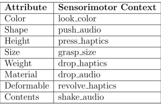
Attribute Chosen Sensorimotor Contexts
Color look color
Shape push audio, look shape
Height press haptics, press audio, squeeze haptics Size grasp size, grasp haptics
Weight drop haptics, hold haptics, lift haptics, push haptics, shake haptics
Material drop audio, push audio Deformable revolve haptics, lift haptics
Contents shake audio, drop haptics, revolve haptics
Table 4.1: Context and Attribute Mappings from the prior experiment to be used for Experiment 2a
(a) look color for Color (b) push audio for Shape and Mate-rial
(c) look shape for Shape (d) press audio for Height
(g) grasp haptics for Size (h) grasp size for Size
(i) hold haptics for Weight (j) lift haptics for Weight and De-formable
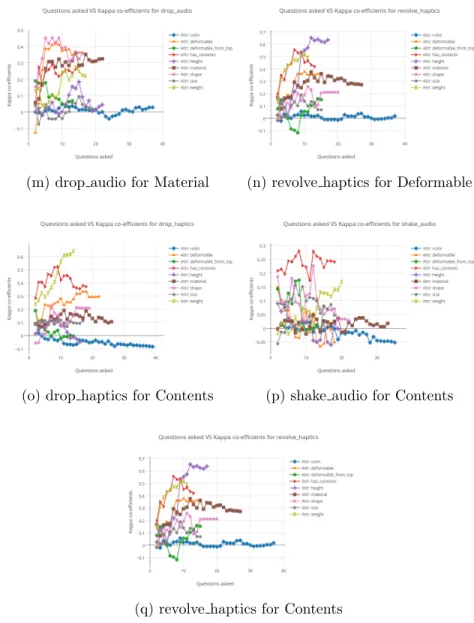
(m) drop audio for Material (n) revolve haptics for Deformable
(o) drop haptics for Contents (p) shake audio for Contents
(q) revolve haptics for Contents
Figure 4.1: The results of the prior experiment carried out to map which contexts are best to learn a particular attribute for Experiment 2a.
4.4.4.2 Experiment 2b: User study with Volunteers
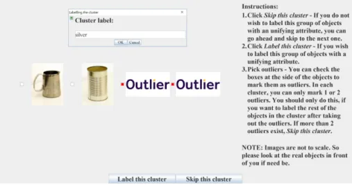
Experiment 2b is conducted to see if our algorithm is robust enough to be used by different users. Different users will have a different understanding on what unifies the cluster and what constitutes a noisy cluster and therefore we would like to see if our algorithm still manages to perform better than the baseline of singly annotating an object in terms of the number of questions asked. For this experiment, we had 18 volunteers (all graduate students from UT Austin), provide us with object attribute labels via a graphical user in-terface as shown in Figure 4.2. The graphical inin-terface displays clusters of objects and asks for attribute labels and follows the same algorithm as Ex-periment 2a except for the part that after each iteration, classifiers are not trained and tested on the test objects. This is because, the ground truth for the test objects will vary from person to person and it does not make sense to test it out with the expert’s ground truth. The aim of this experiment is to get all attribute labels for all objects from different users instead of using the expert’s ground truth table to get our object labels. We are not trying to do classification of novel objects here. However, for the attribute labeling round of the user study, we still do remove 5 objects from the dataset to be able to compare the results of the user study with that of the other experiments.
The volunteers were divided into Groups A and B, each consisting of 9 participants, where Group A provided thecolor, material, weight and size at-tributes and Group B provided theshape, has contents, height anddeformable attributes of the 27 objects. This grouping was done to make the user study
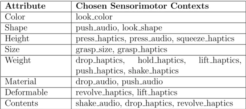
feasible for the participant by reducing the time it took per person to complete the study. Also, as users have to do this experiment in real time, we cannot do all the experiments for every possible context-attribute combination. There-fore, we decided to pick the 8 best contexts to learn the 8 attributes for Ex-periment 2b. These mappings, shown in Table 4.2, were decided based on the results from Experiment 2a. The decision is made based on the highestkappa achieved, the total number of questions asked and also the smoothness of the curve plotted. Plots of contexts which were chosen for a particular attribute are shown in Figure 5.1. The graphs showcase the improvement in kappa as more questions are answered by the expert (more clusters are labelled) for a particular context while learning a specific attribute. Rest of the plots for Experiment 2a can be found in Appendix 1, Section 1.2.
Figure 4.2: Snapshot of the interface used for our user study. User can either label, mark a maximum of two outliers or skip a cluster in each iteration. The category of the attribute label is specified on the top.
Attribute Sensorimotor Context Color look color
Shape push audio Height press haptics Size grasp size Weight drop haptics Material drop audio Deformable revolve haptics Contents shake audio
Chapter 5
Results and Analysis
Rate of Learning Object Attributes: For each of the experiments performed, the rate at which the object attributes were learnt is shown by plotting graphs of the mean number of questions answered against the mean number of training objects labelled. The error bars represent one standard de-viation of uncertainty. The results for the contexts that learnt the attributes best are shown in Figure 5.2. These are also the contexts that were used for Experiment 1, 2a and 2b. The rest of the graphs can be found in the Appendix 1, Section 1.1. The graphs for Experiment 1 are in blue, the ones from Exper-iment 2a w/o Skip Questions are in orange, the ones from ExperExper-iment 2a w/ Skip Questions are in green, the ones from Experiment 2b w/o Skip Questions are in red, the ones from Experiment 2b w/ Skip Questions are in purple. For all contexts, our clustering-based algorithm (Experiment 2a & 2b along with their variations) performs better that baseline of Experiment 1. The rate at which the training objects get labelled for each question answered for Exper-iment 2a & 2b is always much faster than ExperExper-iment 1 except for the color attribute. Forcolor, our algorithm still mostly fares well but not as well as the other attributes. This might be because we use real-world objects and most of them are multi-colored and hence its hard to build single color classifiers
for them. Also, humans tend to classify colors into more sub-categories than any other attribute and hence more questions are required to label all the colors. Many of the user study participants said that they incorporated new categories midway during attribute labelling rounds, leading to more questions being answered and some also made mistakes in picking out outliers, but our algorithm still does better despite that.
Measuring Human Effort: The experiments were carried out to determine how much human effort is required in labeling to learn all attributes for a particular set of objects. We used a multi-modal approach in contrast to the traditional vision approach to ground what each label of each attribute means and building class classifiers for each context using the multi-modal data obtained by the robot via exploring the objects. To measure if our clustering-based approach (Experiment 2a & Experiment 2b) performed better than the usual single object annotations (Experiment 1), we measured the amount of human effort required in the form of number of questions answered by the human during the labeling process. From Figure 5.2, it can be seen that our algorithm learns all the attributes with lesser human effort than the baseline Experiment 1.
To measure how well a context, CBM learned an attribute, AR, the
performance metric used was Cohen’s Kappa coefficient [4] defined as follows:
kappa= P r(c)−P r(e) 1−P r(e)
andP r(e) is the probability that the correct classification occurred by chance. Therefore, Kappa here denotes the level of agreement between the ground truth labels and the label produced by the multi-class classifier for an at-tribute. Kappa is a better performance metric than percentage agreement or percentage accuracy as it takes into consideration chance agreement.
The results are shown in Figure 5.1. Rest of the graphs can be found in Appendix 1, Section 1.2. Note that, Experiment 2b is not part of the plots, askappa is not calculated for Experiment 2b for reasons explained in Section 4.4.4.2. The figure shows the results for the contexts that performed the best for each attribute. and they are chosen based on the highestkappa achieved and also the total number of questions answered to label all the objects. The graphs obtained from Experiment 1 which showcase the baseline results for comparing our clustering-based algorithm are in blue, the one from Experiment 2a w/o Skip Questions are in orange and the ones from Experiment 2a w/ Skip Questions are in green. The error bars provide one standard deviation of uncertainty. In some contexts, the orange and the green graphs completely overlap. This is because no clusters are skipped in the algorithm and hence the count of QS =QN S. For Experiment 1, each object labelled amounts to 1
question being answered. For Experiment 2a, each cluster labelled amounts to 1 question being answered by the expert. As 100 trials were carried out for each context, each data point refers to the mean kappaobtained from all the trials for a particular question count. The graphs also show the standard deviation of the kappa for each question count. Usually for most contexts, the kappa
increases as the number of objects being trained on increases. Some attributes are learnt better than others. For example, height and weight achieve one of the highest kappas while color has the lowest even after training on all 27 objects. This accuracy can be improved in the future by training on more objects and also taking in consideration the issue of having multiple colors in the objects. Also, there is always some noise in the audio, visual and haptic data collected by the robot in the data collection stage and steps could be taken to remove the noise first and then using the cleaned data for clustering. It can be seen that the clustering-based algorithm (Experiment 2a) learns the object labels faster and with lesser human effort than the traditional method of labelling each object (Experiment 1).
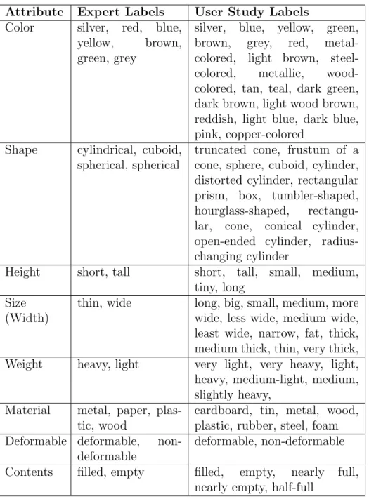
We also look at the variation of labels obtained from Experiment 2b. The different labels obtained for each attribute are tabulated in Table 5.1 which depicts how much they vary from the expert labels and therefore couldn’t be used to train classifier and test against the expert’s labels. However, this is a good way to get an understanding about how robust our algorithm is with different users and our algorithm does fare pretty well.
Attribute Expert Labels User Study Labels Color silver, red, blue,
yellow, brown, green, grey
silver, blue, yellow, green, brown, grey, red, metal-colored, light brown, steel-colored, metallic, wood-colored, tan, teal, dark green, dark brown, light wood brown, reddish, light blue, dark blue, pink, copper-colored
Shape cylindrical, cuboid, spherical, spherical
truncated cone, frustum of a cone, sphere, cuboid, cylinder, distorted cylinder, rectangular prism, box, tumbler-shaped, hourglass-shaped, rectangu-lar, cone, conical cylinder, open-ended cylinder, radius-changing cylinder
Height short, tall short, tall, small, medium, tiny, long
Size (Width)
thin, wide long, big, small, medium, more wide, less wide, medium wide, least wide, narrow, fat, thick, medium thick, thin, very thick, Weight heavy, light very light, very heavy, light, heavy, medium-light, medium, slightly heavy,
Material metal, paper, plas-tic, wood
cardboard, tin, metal, wood, plastic, rubber, steel, foam Deformable deformable,
non-deformable
deformable, non-deformable Contents filled, empty filled, empty, nearly full,
nearly empty, half-full
Table 5.1: Variations in labels obtained per attribute from Experiment 2b with the different users against expert labels used for Experiment 2a.
(a) look color for Color (b) push audio for Shape
(c) press haptics for Height (d) grasp size for Size
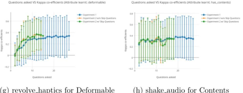
(g) revolve haptics for Deformable (h) shake audio for Contents
Figure 5.1: Graphs depicting thekappa coefficient for each question answered by the expert for a particular context to learn a particular attribute.
(a) look color for Color (b) push audio for Shape
(c) press haptics for Height (d) grasp size for Size
(g) revolve haptics for Deformable (h) shake audio for Contents
Figure 5.2: Graphs depicting the rate of number of training objects labelled per question count for a particular context to learn a particular attribute.
Chapter 6
Conclusion and Future Works
The process of labelling is an essential task that is required for all classification methods. To our knowledge, it is not possible yet to completely take out the human from the picture and labelling remains to be a human-intensive task. Presently, the state-of-the-art is still annotating a single object at a time. Therefore, we introduce our clustering-based approach to reduce the amount of human effort required in labelling. In our framework, the robot learns all the attributes of the objects by asking fewer questions to the human by clustering similar objects together and hence reducing the amount of human effort required in labelling. The robot also grounded the attributes learnt via its multi-modal sensory data and also learnt which multi-sensory context is good for learning a particular attribute. Via the user study, we find that our algorithm is also robust to different users and still fares much better than the baseline.
In the future, we would like to improve the algorithm by incorporating a way to do cluster analysis. This would involve coming up with a metric to calculate the goodness of the clusters formed across all contexts. Currently, there is no inter-cluster interaction when it comes to picking a cluster to be
labelled from a human. We focus only on one context at a time. We only make the decision based on all the clusters from one context. However, in the future, using the cluster analysis metric, we will be able to pick the best cluster that provides the classifier with the best training examples. This way, we need not even use all 27 objects for training and can still get the minimal number of labelled objects to build a good classifier, thereby reducing the amount of human effort required even further. We would like to implement some sort of an active learning technique where only the absolutely needed objects get labelled and are used to do further classification of the remaining objects, an approach similar to the one implemented for image classification in [14] and [15].
The other thing we would like to incorporate is relative category labels. Currently, some of the attributes that are learnt likesmall orbig for learning the attributeheight orlight orheavyfor the attributeweight are usually learnt in reference to some other objects. It is hard to say something is heavy if we do not know what it is being compared against. There was also a general consensus amongst the participants of our user study that relative attributes were much harder to label. Shown a cluster, many a times, they forgot to give a label based on all the objects in the dataset, rather than just considering the cluster in front of them. Also, realistically, as the robot will incrementally get labels for objects it needs to train on, all the objects will not be known beforehand and therefore it does not make sense to base the label of a cluster on all training objects but relative attributes do demand that. Humans are
usually able to make a decision about a relative attribute after multiple inter-actions with objects and in the future, we would like to incorporate that with the robot as well to see how many interactions are required to come up with an accurate label.
Result’s Appendix
1.1
Training Objects VS Questions Answered Graphs
(a) look shape for Shape (b) lift haptics for Deformable
(c) revolve haptics for Contents (d) drop haptics for Contents
(g) push audio for Material (h) grasp haptics for Size
(i) hold haptics for Weight (j) lift haptics for Weight
(k) push haptics for Weight (l) shake haptics for Weight
Figure 1.1: The graphs of the all the other contexts for Experiment 1 and Experiment 2a. The plots showcase the rate of number of training objects labelled per question count for a particular context to learn a particular at-tribute. The error bars give one standard deviation of uncertainty. It can be seen that Experiment 2a performs better than the baseline of Experiment 1 in terms of number of questions answered.
1.2
Kappa Co-efficient VS Questions Answered Graphs
(a) look shape for Shape (b) lift haptics for Deformable
(c) revolve haptics for Contents (d) drop haptics for Contents
(g) push audio for Material (h) grasp haptics for Size
(i) hold haptics for Weight (j) lift haptics for Weight
(k) push haptics for Weight (l) shake haptics for Weight
Figure 1.2: The graphs of the all the other contexts for Experiment 1 and Experiment 2a. The plots showcase the kappa coefficient for each question answered by the expert for a particular context to learn a particular attribute. The error bars give one standard deviation of uncertainty. It can be seen that Experiment 2a performs better than the baseline of Experiment 1 in terms of number of questions answered.
1.3
Context and Attribute Mapping Experiment Graphs
(a) grasp audio (b) hold audio
(c) lift audio (d) poke audio
(g) squeeze audio
Figure 1.3: The graphs of the all the other contexts for the prior experiment which was done to choose which contexts performed best for a particular at-tribute. The plots showcase the kappa coefficient for each question answered and also the total number of questions answered for each attribute. It can be seen that these contexts did not perform well for any of the attributes and hence were not chosen.
Bibliography
[1] Spectral clustering for weka. http://www.luigidragone.com/software/ spectral-clusterer-for-weka/. Accessed: 2015-07-12.
[2] Aitor Aldoma, Zoltan-Csaba Marton, Federico Tombari, Walter Wohlkinger, Christian Potthast, Bernhard Zeisl, Radu Bogdan Rusu, Suat Gedikli, and Markus Vincze. Tutorial: Point cloud library: Three-dimensional object recognition and 6 dof pose estimation. IEEE Robotics & Automa-tion Magazine, 19(3):80–91, 2012.
[3] Gregory Ashby and Todd Maddox. Human category learning. Annu. Rev. Psychol., 56:149–178, 2005.
[4] Jacob Cohen. A coefficient of agreement for nominal scales. Educational and psychological measurement, 20(1):37–46, 1960.
[5] Leslie B Cohen. Commentary on part i: Unresolved issues in infant categorization. 2003.
[6] Dengxin Dai, Mukta Prasad, Christian Leistner, and Luc Van Gool. En-semble partitioning for unsupervised image categorization. Computer Vision–ECCV 2012, pages 483–496, 2012.
[7] Marc O Ernst and Heinrich H B¨ulthoff. Merging the senses into a robust percept. Trends in cognitive sciences, 8(4):162–169, 2004.
[8] Carolina Galleguillos, Brian McFee, and Gert RG Lanckriet. Iterative category discovery via multiple kernel metric learning. International journal of computer vision, 108(1-2):115–132, 2014.
[9] Eleanor J Gibson. Exploratory behavior in the development of perceiv-ing, actperceiv-ing, and the acquiring of knowledge. Annual review of psychology, 39(1):1–42, 1988.
[10] Susan Goldberg, Marion Perlmutter, and Nancy Myers. Recall of re-lated and unrere-lated lists by 2-year-olds. Journal of Experimental Child Psychology, 18(1):1–8, 1974.
[11] Shane Griffith, Jivko Sinapov, Vladimir Sukhoy, and Alexander Stoytchev. A behavior-grounded approach to forming object categories: Separating containers from noncontainers. IEEE Transactions on Autonomous Men-tal Development, 4(1):54–69, 2012.
[12] Mark Hall, Eibe Frank, Geoffrey Holmes, Bernhard Pfahringer, Peter Reutemann, and Ian H Witten. The weka data mining software: an update. ACM SIGKDD explorations newsletter, 11(1):10–18, 2009. [13] Mahmudul Hasan and Amit K Roy-Chowdhury. Context aware active
learning of activity recognition models. In Proceedings of the IEEE In-ternational Conference on Computer Vision, pages 4543–4551, 2015. [14] Prateek Jain and Ashish Kapoor. Active learning for large multi-class
2009. IEEE Conference on, pages 762–769. IEEE, 2009.
[15] Ajay J Joshi, Fatih Porikli, and Nikolaos Papanikolopoulos. Multi-class active learning for image classification. InComputer Vision and Pattern Recognition, 2009. CVPR 2009. IEEE Conference on, pages 2372–2379. IEEE, 2009.
[16] Ravi Kannan, Santosh Vempala, and Adrian Vetta. On clusterings: Good, bad and spectral. Journal of the ACM (JACM), 51(3):497–515, 2004.
[17] Ashish Kapoor, Kristen Grauman, Raquel Urtasun, and Trevor Darrell. Active learning with gaussian processes for object categorization. In Computer Vision, 2007. ICCV 2007. IEEE 11th International Confer-ence on, pages 1–8. IEEE, 2007.
[18] Aleˇs Leonardis and Sanja Fidler. Learning hierarchical representations of object categories for robot vision. InRobotics Research, pages 99–110. Springer, 2010.
[19] David Liu and Tsuhan Chen. Unsupervised image categorization and object localization using topic models and correspondences between im-ages. In Computer Vision, 2007. ICCV 2007. IEEE 11th International Conference on, pages 1–7. IEEE, 2007.
[20] Lu´ıs Seabra Lopes and Aneesh Chauhan. Scaling up category learning for language acquisition in human-robot interaction. In Proceedings of
the Symposium on Language and Robots, pages 83–92. Citeseer, 2007. [21] Dermot Lynott and Louise Connell. Modality exclusivity norms for 423
object properties. Behavior Research Methods, 41(2):558–564, 2009. [22] Zoltan Csaba Marton, Radu Bogdan Rusu, Dominik Jain, Ulrich Klank,
and Michael Beetz. Probabilistic categorization of kitchen objects in table settings with a composite sensor. InIROS, pages 4777–4784, 2009. [23] Cynthia Matuszek, Nicholas FitzGerald, Luke Zettlemoyer, Liefeng Bo, and Dieter Fox. A joint model of language and perception. InProceedings of the 29th International Conference on Machine Learning, Edinburgh, Scotland, UK, 2012.
[24] Rachel Melkman, Barbara Tversky, and Daphna Baratz. Developmen-tal trends in the use of perceptual and conceptual attributes in group-ing, clustergroup-ing, and retrieval. Journal of experimental child psychology, 31(3):470–486, 1981.
[25] Sabina Pauen. Evidence for knowledge–based category discrimination in infancy. Child Development, 73(4):1016–1033, 2002.
[26] Thomas G Power. Play and exploration in children and animals. Psy-chology Press, 1999.
[27] Radu Bogdan Rusu, Nico Blodow, and Michael Beetz. Fast point feature histograms (fpfh) for 3d registration. InRobotics and Automation, 2009.
ICRA’09. IEEE International Conference on, pages 3212–3217. IEEE, 2009.
[28] Burr Settles. Active learning literature survey. University of Wisconsin, Madison, 52(55-66):11, 2010.
[29] Jianbo Shi and Jitendra Malik. Normalized cuts and image segmenta-tion. IEEE Transactions on pattern analysis and machine intelligence, 22(8):888–905, 2000.
[30] Jivko Sinapov, Connor Schenck, Kerrick Staley, Vladimir Sukhoy, and Alexander Stoytchev. Grounding semantic categories in behavioral in-teractions: Experiments with 100 objects. Robotics and Autonomous Systems, 62(5):632–645, 2014.
[31] Jivko Sinapov, Connor Schenck, and Alexander Stoytchev. Learning re-lational object categories using behavioral exploration and multimodal perception. In Robotics and Automation (ICRA), 2014 IEEE Interna-tional Conference on, pages 5691–5698. IEEE, 2014.
[32] Jivko Sinapov and Alexander Stoytchev. Object category recognition by a humanoid robot using behavior-grounded relational learning. In Robotics and Automation (ICRA), 2011 IEEE International Conference on, pages 184–190. IEEE, 2011.
[33] Beate Sodian, Wolfgang Schneider, and Marion Perlmutter. Recall, clus-tering, and metamemory in young children. Journal of Experimental
Child Psychology, 41(3):395–410, 1986.
[34] Sudheendra Vijayanarasimhan and Kristen Grauman. Large-scale live active learning: Training object detectors with crawled data and crowds. International Journal of Computer Vision, 108(1-2):97–114, 2014.
[35] Carl Vondrick and Deva Ramanan. Video annotation and tracking with active learning. In Advances in Neural Information Processing Systems, pages 28–36, 2011.
[36] Maggie Wigness, Bruce A Draper, and J Ross Beveridge. Selectively guiding visual concept discovery. In Applications of Computer Vision (WACV), 2014 IEEE Winter Conference on, pages 247–254. IEEE, 2014. [37] Maggie Wigness, Bruce A Draper, and J Ross Beveridge. Efficient label collection for unlabeled image datasets. InProceedings of the IEEE Con-ference on Computer Vision and Pattern Recognition, pages 4594–4602, 2015.
[38] Ian H Witten, Eibe Frank, Mark A Hall, and Christopher J Pal. Data Mining: Practical machine learning tools and techniques. Morgan Kauf-mann, 2016.
Vita
Priyanka Khante was born in Mumbai, India on 7 April, 1993. She is the daughter of Milind G. Khante and Ujwala M. Khante. She received the Bachelor of Science degree from Stony Brook University in May 2014. She decided to pursue her graduate studies in order to learn about robots in real-world environments and joined University of Texas at Austin in August 2014. Since then, she worked with Dr. Peter Stone in the Building Wide Intelligence (BWI) Lab. This thesis is a summary of the subset of work performed from Fall 2015 to Spring 2017.
Permanent address: [email protected]
This thesis was typeset with LATEX† by the author.
†LATEX is a document preparation system developed by Leslie Lamport as a special version of Donald Knuth’s TEX Program.