methods
Jason F. Ralph,1,∗ Simon Maskell,1,† and Kurt Jacobs2, 3, 4,‡
1Department of Electrical Engineering and Electronics, University of Liverpool, Brownlow Hill, Liverpool, L69 3GJ, UK. 2
U.S. Army Research Laboratory, Computational and Information Sciences Directorate, Adelphi, Maryland 20783, USA. 3
Department of Physics, University of Massachusetts at Boston, Boston, MA 02125, USA 4Hearne Institute for Theoretical Physics, Louisiana State University, Baton Rouge, LA 70803, USA
(Dated: October 12, 2017)
This paper proposes an efficient method for the simultaneous estimation of the state of a quan-tum system and the classical parameters that govern its evolution. This hybrid approach benefits from efficient numerical methods for the integration of stochastic master equations for the quantum system, and efficient parameter estimation methods from classical signal processing. The classical techniques use Sequential Monte Carlo (SMC) methods, which aim to optimize the selection of points within the parameter space, conditioned by the measurement data obtained. We illustrate these methods using a specific example, an SMC sampler applied to a nonlinear system, the Duff-ing oscillator, where the evolution of the quantum state of the oscillator and three Hamiltonian parameters are estimated simultaneously.
PACS numbers: 05.45.Mt, 03.65.Ta, 05.45.Pq
Keywords: quantum state-estimation, continuous measurement, classical parameter estimation, sequential Monte Carlo methods
I. INTRODUCTION
Stochastic master equations provide a model for the evo-lution of open quantum systems subject to continuous measurements [1–3]. The trajectories that the stochas-tic master equations generate represent the evolution of the state of an individual quantum system, conditioned on a particular measurement record. In theoretical stud-ies, the measurement record is a simulated sequence cor-responding to a particular realization of the evolution. However, recent experiments that implement continu-ous quantum measurements have demonstrated that the evolution of individual quantum systems can be recon-structed from experimental data [4–7]. The generation of such trajectories in real time during the measure-ment process will be an important step towards state-dependent feedback control of individual quantum sys-tems [1–3]. Feedback control has been demonstrated in quantum systems using the output measurement record as an input signal to the control system in optical [8, 9], opto-mechanical [10–12], and mesoscopic superconduct-ing systems [13, 14]. In most of these examples, while the direct use of the measurement record in the control sys-tem demonstrates the utility of quantum feedback con-trol, it is limited by the fact that the evolution of the un-derlying state of the system is not included in the genera-tion of the controls. State-dependent control is more flex-ible and can include quantities that are estimated from,
∗Electronic address: [email protected] †Electronic address: [email protected] ‡Electronic address: [email protected]
but are not directly measured in experiments.
Given a measurement record, a Stochastic Master Equation (SME) provides an estimate of the quantum state at each point in time, and – in the case of mixed states – an indication of the uncertainty associated with this state in terms of an estimate of its purity. The SME is derived by taking a single quantum system and cou-pling it weakly to environmental degrees of freedom that mediate a continuous measurement process. The con-tinuous measurement of the coupled system is realized by continuously measuring the state of the environment, which can be modeled as a sequence of projective mea-surements on successive environmental degrees of free-dom. The simplest example of this process is the mea-surement of the electromagnetic radiation emitted by the system, in which case the environment is the electromag-netic field [2, 3]. In the most common form of the SME, a Markovian condition is applied, meaning that the en-vironment carries information away from the system but does not by itself feed this information back to affect the system at a later time. The resulting evolution of the system is continuous and stochastic, with the stochastic term arising from the effect of the sequence of measure-ments on the combined system.
In simulations, an SME is used to analyze the proper-ties of an open system under the action of a continuous se-quence of measurement operators, using a realization for the noise process and calculating the evolution of the sys-tem conditioned on this realization. When interpreting experiments, the SME is used to reconstruct the estimate of the quantum state as a function of time from the given measurement record provided by the experiment. In this regard, the SME is very similar to classical state estima-tion techniques (often referred to as ‘target tracking’ or
‘object tracking’ [32–34]), which are used to interpret se-quences of classical noisy sensor measurements to form a coherent picture of the world. These classical techniques have been developed to interpret sensor data (radar or sonar signals, and sequences of images) where objects are moving against noisy backgrounds. The motion of the objects may be unpredictable or uncooperative, their identity may not be known from the measurements, they may be occluded for periods of time, and individual ob-jects may not be fully resolved by the sensor. Classical state estimation techniques provide methods to solve all of these problems and ambiguities.
With a continuous quantum measurement, the mea-surement record contains information about the evolu-tion of the particular quantum state (a quantum trajec-tory) but the properties of this trajectory also contain information about the classical parameters that govern the dynamics of the system: the classical parameters in the Hamiltonian and the strength of the coupling to the environment. In this paper, we demonstrate how the stochastic master equation can be augmented with tech-niques drawn from classical state estimation, Sequential Monte Carlo (SMC) methods, to estimate several Hamil-tonian parameters efficiently alongside the quantum tra-jectories.
We begin our presentation by first reviewing other ap-proaches to Hamiltonian parameter estimation, and the development of a set of Hybrid SMEs for the quantum evolution and the Kushner-Stratonovich equation for the classical parameters [15] in sections II and III, respec-tively. In section IV, we then discuss how efficient classi-cal parameter estimation techniques [16] can be applied to the solution of the classical aspects of the Hybrid SME. Section V introduces an example system, the Duffing os-cillator, which contains a number of relevant experimen-tal parameters, and Section VI presents results for the simultaneous estimation of the quantum trajectories for the oscillator and up to three Hamiltonian parameters. Section VII discusses how such methods may be useful in practical systems and draws conclusions from the results presented.
II. HAMILTONIAN PARAMETER
ESTIMATION
The problem of estimating the dynamical parameters of a quantum system has been studied previously by a number of authors, including those who have adopted a continuous measurement approach. This estimation pro-cess is often referred to as Hamiltonian parameter esti-mation. This is because the basic description of quantum dynamics is encapsulated by the Hamiltonian operator, which determines the equations of motion, and values of the classical parameters in the Hamiltonian determine the specifics of the evolution.
A standard method for determining the dynamics of a quantum system is to prepare it many times in a range
of different initial states, allow it to evolve, and then measure it before re-preparation. The results of the measurements can then be combined in a tomographic-like process to obtain the equation of motion for linear Schr¨odinger evolution [17]. An alternative approach, and the one in which we are interested here, is to prepare the system only once and to continually monitor its subse-quent evolution to build a picture of its dynamics. A full description of the problem involves starting with a prior probability density for the parameters one wishes to determine and then using Bayes’ theorem to contin-ually update this probability density from the stream of measurement results as they are obtained. A number of authors have considered this problem [15, 18–28]. This is of particular interest when the parameters of a system change slowly with time, and one wishes to be able to track the variations in the parameters. It is also rele-vant to the problem of using quantum systems as probes to measure time-varying classical fields (such as gravity waves [29] and magnetic fields [30]), as these fields appear as parameters in the Hamiltonian.
As discussed in the introduction, a dynamical equation referred to as the stochastic master equation (SME) can be used to track the evolution of a quantum system from the results of a continuous measurement so long as the dynamical parameters of the system are known. If they are not known then the full estimation problem involves both the SME and a Kushner-Stratonovich equation that evolves the probability density for the parameters of the system. The combined set of dynamical equations has been referred to as aHybrid SME[15]. The first papers on the subject of Hamiltonian parameter estimation via continuous measurements were concerned mainly with deriving the Hybrid SME and applying it to the estima-tion of a single parameter [18, 19]. Subsequently, Tsang and collaborators considered the more general problem of smoothing in which a time-varying parameter (a signal or wave-form) is estimated from all the measurement re-sults obtained, and determined the ultimate limits to this procedure [21–24, 26]. An alternative and interesting ap-proach to the problem was proposed recently by Bassaet al. [27]. While most of the related work on parameter estimation employs continuous measurements, this ap-proach considered a sequence of instantaneous measure-ments, and employed a discrete version of the Hybrid SME where several classical parameter values were en-coded in an expanded quantum state.
A major problem with the Hybrid SME is that it is highly demanding from a computational point of view; in order to evolve the Kushner-Stratonovich equation for the probability density describing the observer’s knowl-edge of the parameters, the SME must be evolved for every value of the parameters for which this density is appreciable. The grid of points for which the SME must be evolved becomes large very quickly as the num-ber of parameters increases. Two previous papers have put forward methods aimed at addressing this difficulty. Ralphet al.[15] and Cortezet al.[28] considered the
es-timation of a single frequency parameter, and presented methods to bypass the Kushner-Stratonovich equation. These papers estimate the natural oscillation frequency of a qubit directly from the measurement record. This approach has many benefits in terms of computational efficiency, but it has the disadvantage of not providing a simultaneous estimate of the quantum state of the sys-tem – which would be provided by the full solution of the Hybrid SME. Here, we will explore the use of a po-tentially more powerful technique in which the proba-bility density is replaced with a finite set of samples of the parameters that are evolved instead. The examples given below typically use 50-100 quantum states and the equivalent of thousands to millions of classical parame-ter values. The purpose is again to reduce the number of copies of the quantum state that must be evolved in parallel using the SME, but we will apply this method to the challenging problem of estimating multiple parame-ters simultaneously.
III. HYBRID STOCHASTIC MASTER EQUATIONS
The simultaneous estimation of the quantum state of a system and the classical Hamiltonian parameters that govern its evolution was considered in Ref. [15], where an approach was presented based on a set of parallel SMEs, each using a different set of parameter values contained in a vectorλ, which have an associated probability. The final mixed state is then constructed by averaging over the probabilities for the classical parameters. The prob-abilities associated with the different parameter vectors evolve via a Kushner-Stratonovich equation and are con-ditioned on the continuous measurement record [15].
For a quantum system subject to a continuous mea-surement, with a known set of Hamiltonian parameters, the evolution of the quantum state,ρc(t), conditioned on the measurement record, y(t), is given by the stochas-tic master equation [1–3]. In general, the interaction with the environment can be represented by a set of sys-tem operators which are coupled to environmental de-grees of freedom, some of which are not measured ˆVj (j= 1. . . m) (‘unprobed’ operators), and some of which are measured and generate the continuous weak measure-ment ˆLr(r= 1. . . m0). In an ideal case, the measurement record is 100% efficient, with all of the available infor-mation being reflected in the measurement record. Un-fortunately, real measurements are rarely ideal and the continuous measurement record is often corrupted with extraneous (classical) noise sources. These extraneous degrees of freedom can be characterized by an efficiency parameter for the measurement operators, ˆLrhas an effi-ciencyηr. Specifically,ηris the fraction of the total noise power due to the quantum measurement as opposed to power contained in the other extraneous noise sources.
For unprobed operators ˆVrand measurement operators ˆ
Lr, the general form for the SME is given by,
dρc = −i h ˆ H, ρc i dt + m X j=1 ˆ VjρcVˆj†− 1 2 ˆ Vj†Vˆjρc+ρcVˆj†Vˆj dt + m0 X r=1 ˆ LrρcLˆ†r− 1 2 ˆ L†rLˆrρc+ρcLˆ†rLˆr dt + m0 X r=1 √ ηr ˆ Lrρc+ρcLˆ†r−Tr( ˆLrρc+ρcLˆ†r) dWr (1)
where ˆH is the Hamiltonian of the system, dt is an in-finitesimal time increment, and the measurement record for each of the measurement operators ˆLr during a time stept →t+dt is given by, y(t+dt)−y(t) =dyr(t) = √
ηjTr( ˆLrρc +ρcLˆ†r)dt +dWr. We will take dWr to be a real Wiener increment such that dWr = 0 and
dWrdWr0 =δrr0dt for simplicity, but this is not strictly
necessary. More general forms of complex increments may also be used [35].
Where the evolution of a quantum system is governed by a set of Hamiltonian parameters that are not known exactly, we can describe the parameters in terms of a classical probability density,P(λ), whereλ= (λ1, λ2, ...). The system is then described by a set of SMEs, one for each set of possible parameter values,
dρc,λ = −i h ˆ H(λ), ρc,λ i dt + m X j=1 ˆ Vjρc,λVˆj†− 1 2 ˆ Vj†Vˆjρc,λ+ρc,λVˆj†Vˆj dt + m0 X r=1 ˆ Lrρc,λLˆ†r− 1 2 ˆ L†rLˆrρc,λ+ρc,λLˆ†rLˆr dt + m0 X r=1 √ ηr ˆ Lrρc,λ+ρc,λLˆ†r −Tr( ˆLrρc,λ+ρc,λLˆ†r)dWr (2)
The evolution of the probability density P(λ) is gov-erned by a Kushner-Stratonovich stochastic differential equation, derived in [15] for a single efficient measure-ment operator and in the absence of additional unprobed environmental operators. Any unprobed environmental operators affect the evolution of the individual SMEs but they do not play a role in the evolution of P(λ). How-ever, the equation given in [15] generalizes naturally to include measurement inefficiencies and is given by,
dPr(λ) = √ ηr(Tr( ˆLrρc,λ+ρc,λLˆ†r)−Tr( ˆLrρc+ρcLˆ†r)) ×(dyr(t)− √ ηrTr( ˆLrρc+ρcLˆ†r)dt)P(λ) (3)
wheredPr(λ) is the update to the probability density due to a measurement incrementdyr(t) corresponding to the
measured operator ˆLr, such that P(dyr(t)|λ) = e(−(dyr(t)− √ ηTr( ˆLrρc,λ+ρc,λLˆ†r))2/dt) √ 2πdt (4)
and the full conditional density matrixρc is given by,
ρc= Z
λ
P(λ)ρc,λdλ (5)
IV. SEQUENTIAL MONTE CARLO METHODS
Sequential Monte Carlo methods originate in the field of multi-target tracking [31]), but have been adopted and generalized to form a set of very efficient methods for pa-rameter and state estimation in classical signal process-ing and nonlinear filterprocess-ing. SMC methods are sometimes referred to asparticle filters, but particle filters are a spe-cial case of the general approach. An SMC method relies on the approximation of a continuous probability distri-bution by a finite set of points (or particles) which ple the parameter space. The importance of each sam-ple point changes in response to (is conditioned by) the measurements associated with the parameters being esti-mated, and the sample points can be periodically resam-pled to concentrate sampling towards regions of higher relative probability.
In particle filters, the sample points are allowed to evolve according to some dynamical process, generating a time dependent history or a track within the param-eter space. In the example presented in this paper, the parameters are selected to be constant and another SMC method is more suitable. We adopt an approach used recently for parameter estimation in classical differen-tial equations [16], which is an example of a
Sequen-tial Monte Carlo sampler. This approach is particularly
well-suited to the estimation of fixed parameters; how-ever, the SMC sampler used here still embodies all of the key features of a general SMC method: sampling, con-ditioning/updating, and resampling. A number of very approachable tutorials and introductions to particle fil-ters and general SMC methods have been published. For example, a comprehensive guide to SMC methods and their applications is available in [36], a mathematical in-troduction is given in [37], and a widely cited tutorial to particle filters and SMC methods is contained in [38].
Formally, an SMC method approximates a (classical) expectation for a functionh(x) over a probability distri-bution p(x) defined on some parameter space Λ, x∈Λ, given by
¯
h= Z
h(x)p(x)dx
using a finite sum of a set of points x(i) (i = 1. . . N) drawn from p(x), which is known as the target distribu-tion. The expectation value for an arbitrary function can
be approximated by, ¯ h' 1 N N X i=1 h(x(i))
The larger the number of sample points, the better the approximation – in fact, under reasonable assumptions, the variance of the error in ¯hcan be shown to scale as 1/N in any number of dimensions [39]. The problem is that, in most practical cases, the probability distribution is unknown. It needs to be estimated from a sequence of measurements. To do this, another distribution, the
proposal distributionq(x), is introduced such that [37],
¯ h = Z h(x)q(x)p(x) q(x)dx= Z h(x)q(x)w(x)dx ' N X i=1 w(i) PN j=1w(j) h(x(i)) (6)
where w(x) = p(x)/q(x) and the w(i)’s are (unnormal-ized) weights associated with each sample point. In our case, each sample point is associated with a parameter value or a vector of values for each of the parameters be-ing sought, w(i) ↔ λ(i), where λ(i) ∈ Λ. Initially, the sample points are randomly selected from a prior dis-tribution, which covers the entire range of possible pa-rameter values, and are given a uniform weight. As new measurements are added, the accuracy of the estimated quantity ¯h is improved by updating the weights associ-ated with the particles to reflect the new information that the measurement contains. Some weights are increased and some weights are reduced when the measurement supports or contradicts the corresponding sample point, respectively.
The valuesw(i)are referred to as ‘weights’ rather than probabilities because, although they are related to prob-abilities, they are not necessarily normalized after each time step and do not necessarily sum to one. In prac-tice, it is convenient to normalize the weights after each time step. Here, we denote the normalized weights by
˜
w(i) [16]. When sample points have very low weight, and hence very low probability, they can be removed and replaced with alternative particles, but this resampling process must be done carefully so as to ensure that the statistical quantities remain unbiased and will converge efficiently to the desired values.
The proposal distribution should be simple to calculate and different choices ofq(x) are used in different variants of the SMC approach [36–38]. The secret to working with SMC methods is to pick a suitable proposal distribution to solve the problem in a robust manner using limited computational resources. In particular, a good choice of proposal distribution allows classical parameters to be estimated significantly more efficiently than when using an enumerative or grid based method [38], as was used for a one parameter Hybrid SME problem in [15, 27].
For our Hybrid SME problem, we start by selecting an initial set of sample points in the parameter space
using a prior distribution and initialize an SME (2) for each of the sample points. For the examples shown be-low, the quantum state of the system is initialized to be a thermal mixed state, and the prior distribution is cho-sen to be uniform over some finite range within which the true parameter values are known to lie. An accu-rate initial prior distribution can significantly reduce the number of particles required by the SMC sampler, but in many situations the prior is not well defined. Once the points have been selected, the weights are initialized withw(0i)= ˜w(0i)= 1/N.
For each time step, the individual SMEs are integrated using the increment (2) found using the parameter value
λ(i) associated with the particle. A corresponding mea-surement probability is found from (4) and used to up-date the (unnormalized) particle weight wk−(i)1,r → w(k,ri)
using [16]
wk,r(i) =p(dyr(tk)|λ(i))w (i)
k−1,r (7) for thek’th measurement from measurement operator ˆLr at timetk. All particles are updated after the measure-ment incremeasure-ment and then weights are normalized.
Resampling to generate new particles only occurs when the distribution of weights amongst the particles is such that the effective sample size (or the effective number of particles)Nef f = 1/(Pi( ˜w
(i))2) falls below some thresh-old value – indicating that the weight is being concen-trated in a relatively small number of particles and a sig-nificant number of particles have low weight and do not contribute to the estimates; a problem known in the SMC literature assample impoverishmentorweight degeneracy
[37]. It is known that the variance of the weight distri-butions across different realizations of the SMC sampler is guaranteed to grow with each time step [38]. However, since a given realization (i.e. one run of the algorithm) does not have access to the ensemble of all possible real-izations, it is convenient to monitor something that can be computed from a single realization. The effective sam-ple size is well established as such a quantity [40] and it can be considered to be a noisy measurement of the (in-verse of the) variance. Between resampling events, the variance of the weight distributions will (on average) in-crease and the effective sample size will dein-crease. While the precise threshold value used is a somewhat arbitrary choice for the algorithm designer, it is common (across the vast range of applications of SMC samplers and par-ticle filters) to consider threshold values between N/10 and N/2. In the cases shown below the threshold value forNef f was set to beN/2 [16].
When the particles are resampled, the new candi-date values ˜λare sampled from the distribution formed from the current particle weights. The particles with the highest weights are more likely to be selected, al-though the particles with relatively low weights still have a chance of being selected. The new particle pa-rameter values are then selected using the distribution
q(˜λ|λ(i)) =N(˜λ;λ(i),Σ), where N(x;µx, S) is a normal
distribution with mean µx and covariance S, and Σ is related to the covariance matrix associated with the cur-rent particle weights, Σk. The role ofq(˜λ|λ(i)) is to select new points, ˜λ(i), around the current particles with large weights, but not at exactly the same point. In this pa-per, we use a defensive strategy [16, 41], where 90% of resampled points use a covariance which is 10% of the current covariance, Σ = 0.1Σk, and 10% of the resam-pled points use the full covariance matrix Σ = Σk. This allows for small perturbations in parameter space around the high weight sample points, including the correlations between different parameters seen in the covariance ma-trix, and a small number of large excursions, to explore more of the parameter space than is currently being cov-ered by the sample points with large weight. There are two specific design considerations relevant to the choice of the distribution,q. The first is to ensure that having more samples will give rise to more accurate estimates of quantities of interest, which is manifest empirically as robustness. Put simply, this demands that samples are proposed in a way that explores possible but potentially low probability states. The second is to ensure that the SMC method is computationally efficient, i.e. that it gets as accurate an estimate as is possible with a given num-ber of samples. This demands that samples are placed in high probability areas. A defensive proposal is an ad-vanced, but relatively standard technique, used in parti-cle filters and SMC samplers, that combines robustness with efficiency by having two elements to the proposal, one that is designed to ensure the sampler is robust and the other that is designed to ensure that it is efficient.
When the new sample points have been selected, they are initially assigned the weight ˇw(0i) = 1/N and then the unnormalized weight for the new candidate points is calculated reusing the entire record of measurement increments, ˇ wk(i)= Q r,kp(dyr(tk)|λ˜ (i) ) Q r,kp(dyr(tk)|λ(i)) ˇ w0(i) (8)
Once all of the new weights have been recalculated they can be renormalized, and the integration of the Hybrid SME can continue as normal. Where the new sample weights are still degenerate and the effective number of particles is still below the threshold value, the resampling (and recalculation) needs to be performed again.
To summarize, the SMC method used here can be de-scribed in the following five steps:
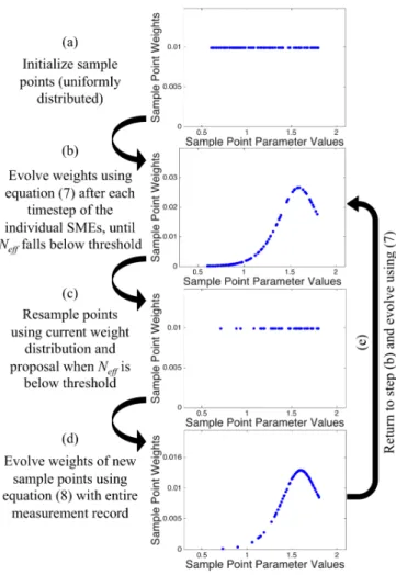
(a) Initialize the individual density matricesρc,λ(i) using
thermal mixed states, and select a set of classical pa-rameter values (sample points or particles)λ(i)using a uniform distribution covering the full range of pos-sible parameter values, and assign uniform weights to each of these ˜w0(i)= 1/N.
(b) Evolve the quantum state using the individual SMEs (2), using the corresponding classical parameters and
FIG. 1: (Color online) Schematic process, showing the main steps in the SMC Sampler for a one parameter example.
updating their weights using (7). Continue this evo-lution until Nef f drops below the threshold value. (c) If Nef f is below the threshold value, the classical
parameter values are resampled using a cumulative probability distribution calculated from the particle weights. This resampling creates a new set of par-ticles/sample points, where the classical parameters are selected around the ‘parent’ values. The defen-sive strategy introduces small perturbations around the parent values and the occasional large perturba-tion to explore a wider parameter space – the new weights associated with each of the new parame-ter values/sample points are uniformly distributed at this point.
(d) Once the new values have been selected, the com-plete evolution of each quantum state is recalculated using new initial thermal states and the individual SMEs (using the same measurement record), and the uniform weights from step (c) are recalculated using (8).
(e) Return to step (b) with evolution of the quantum state and weights determined by the individual SMEs
and the weight update (7), until Nef f drops below the threshold value again, at which point the resam-pling step (c) and the re-weighting step (d) are again required.
A schematic example of the estimation process for a one dimensional parameter example is shown in Figure 1. In this example, it is possible to see that the initial uniform weighting of the particles evolves so that the relatively large number of particles below a parameter value of 1.0 carry very little weight, and the distribution of particles immediately after resampling is concentrated more to-wards the values above 1.0. The re-weighted parameter values shown in (d) represent a better approximation to the underlying probability distribution than those shown in (b), which contains significant gaps towards the peak of the distribution. For a more detailed description of the implementation, a full description of the SMC method is given as pseudo-code in [16].
The recalculation over the entire measurement history is an unfortunate, but necessary, computational cost in the SMC sampler. Recalculating the weights for the en-tire history of measurement increments will often take a significant amount of time. However, the need to regu-larly resample the entire set of particles reduces as the distribution of the particles improves to reflect the infor-mation contained in the measurements [16]. This means that the computational load introduced is biased towards the start of the calculation of a quantum trajectory. In addition, for resampled points very close to the parent particles, some approximations are possible based on the fact that the ratio between the products in (8) is very close to one. It is not possible to remove the recalcula-tion entirely however without constraining the resampled parameter values and therefore not exploring the full pa-rameter space.
V. EXAMPLE SYSTEM – DUFFING
OSCILLATOR
The properties of the quantum trajectories generated by the Duffing oscillator have been studied extensively in terms of the appearance of chaotic behavior from quan-tum systems in the classical limit [42–52], but it is also a model used for a number of other practical systems where quantum effects in classical nonlinear systems are of interest. For example, it has been used to describe the motion of a levitated particle in an electromagnetic trap [53, 54], and is the basis for the analysis of the properties of vibrating beam accelerometers [55–57]. The Hamilto-nian for the Duffing oscillator can be written in the gen-eral form, using dimensionless position and momentum operators ˆqand ˆp, ˆ H(λ) = 1 2pˆ 2+1 2ω 2qˆ2+1 4µqˆ 4+gcos(t)ˆq+Γ 2(ˆqpˆ+ ˆpqˆ) (9) where the vectorλ= (ω, µ, g) contains the three Hamil-tonian parameters of interest: the natural (linear)
oscil-lation frequency ω, the nonlinear coefficient µ, and the strength of the external driving term g. The measure-ment is applied via a Linblad operator ˆL =√2Γˆa, and ˆ
a is the harmonic oscillator lowering operator so that ˆ
q = (ˆa†+ ˆa)/√2 and ˆp=i(ˆa†−aˆ)/√2 with [ˆa,ˆa†] = 1 and ~ = 1. We fix the measurement strength so that
Γ = 0.125 for all of the results presented here. The final term in the Hamiltonian is included because, in combination with the dissipative measurement process, it generates linear damping in momentum. This is a use-ful numerical addition because it keeps the phase space contained, thereby restricting the numbers of states re-quired in the simulation, without affecting the underlying physics.
The numerical integration of the individual SMEs uses a method developed by Rouchon and colleagues [58, 59] specifically for stochastic master equations. This method has been demonstrated to provide significant benefits in terms of accuracy versus computational resources when compared to standard methods, such as Milstein’s method [60], for both systems involving small numbers of basis states [59] and large numbers of basis states [61]. We also employ a moving basis method used by Schack, Brun and Percival [42, 43] to shift basis states to be cen-tred on the current expectation value of the state. Al-though not strictly necessary [42, 43], we shift the basis after each time step. This comes at a computational cost but it also ensures that the number of basis states em-ployed is minimized. Once the evolution of the individual SMEs has been calculated, using the appropriate set of parameters, the combined density operator is calculated by averaging over all of the individual states, weighted appropriately by the particle weights.
The increment to the stateρ(cn,λ)for the time step from
tn =n∆tto tn+1= (n+ 1)∆tis calculated using ρ(cn,λ+1)= ˆ Mn,λρ (n) c,λMˆ † n,λ+ (1−η) ˆLρ (n) c,λLˆ †∆t TrhMˆn,λρ (n) c,λMˆ † n,λ+ (1−η) ˆLρ (n) c,λLˆ†∆t i (10)
where ∆ρ(cn,λ)=ρc(n,λ+1)−ρ(cn,λ) and ˆMn,λ is given by
ˆ Mn,λ = I− iHˆ +1 2 ˆ L†Lˆ ∆t+η 2 ˆ L2(∆W(n)2−∆t) +√ηLˆ√ηTr[ ˆLρ(cn,λ)+ρ(cn,λ)Lˆ†]∆t+ ∆W(n)
where the ∆W’s are independent Gaussian variables with zero mean and a variance equal to ∆t. Once the incre-ment has been calcluated, center of the basis is moved to the new location of the state in phase space, as given by the expectation values of the phase space operators, (q(n+1),λ, p(n+1),λ) = (Tr[ˆqρ (n+1) c,λ ],Tr[ˆpρ (n+1) c,λ ]), using the displacement operator [42, 43], ˆ D(p(n+1),λ, q(n+1),λ) = exp i(p(n+1),λqˆ−q(n+1),λpˆ) (11)
and the conditioned state in the shifted basis is given by
ρ(cn,λ+1)→Dˆ(p(n+1),λ, q(n+1),λ)ρ (n+1)
c,λ Dˆ(p(n+1),λ, q(n+1),λ)† (12)
VI. RESULTS
The Duffing Hamiltonian (9) has four classical param-eters but we will fix the measurement strength so that Γ = 0.125 and we will concentrate on the estimation of the other three parameters: the linear oscillator fre-quency ω, the coefficient of the nonlinear term µ, and the magnitude of the drive termg. The estimated val-ues for these three parameters are denoted by ˜ω, ˜µ, and ˜
grespectively. For all of the examples shown below, the actual values for parameter values were set to beω= 1.2,
µ= 0.15, andg = 3.0. The numerical integration of the SMEs was performed using time steps ∆t = 2π/500 so that there were 500 steps per period of the drive term. The individual SMEs for each particle/sample point used a moving basis with 15 harmonic oscillator states, and the composite state was calculated by combining the density matrices from the individual SMEs using (5), using a moving basis with 60 harmonic oscillator states.
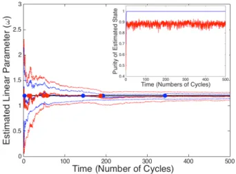
Figure 2 shows two examples for the estimation of the linear oscillator frequency ˜ω. The examples correspond to the same stochastic record (i.e. the same realization) but with different measurement efficiencies. The blue lines correspond to the case where the measurement is 100% efficient (with η = 1). This shows a rapid con-vergence to the actual value,ω = 1.2, within about 50-100 periods/cycles of the drive term. The 3 sigma er-rors predicted for the estimate are also shown, together with the resampling events as blue circles. The conver-gence is fairly rapid and the estimate is relatively stable once converged. The red line on the same figure shows an example where the measurement is inefficient, corre-sponding to a measurement efficiency of 40% orη = 0.4 (chosen to match the estimated efficiency reported in [5]). In this case, the convergence is much slower, indicating that the measurement record contains less information upon which a parameter estimate can be constructed. In this case, the estimated parameter value only stabi-lizes after around 150-200 cycles of the drive term, and the larger estimated errors indicate this increased uncer-tainty. In both cases shown, there are slight variations in the estimated values (seen around 200-250 cycles) but these are relatively small and are well within the esti-mated errors. In addition, where the estimation process takes longer, the number of resampling events (red cir-cles) tends to increase and they often occur later in the process than the corresponding resampling events for effi-cient measurements, leading to increased computational demands to recalculate the weights after resampling. In addition to the estimates, Figure 2 also shows the pu-rity of the full estimated quantum state for both cases as an inset. For efficient measurements, the conditioned
quantum state purifies very rapidly (1-2 periods of the drive term) and remains pure throughout the estimation process. For inefficient measurements, the conditioned quantum state purifies somewhat but then the purity fluctuates between 0.8 and 0.9. The state remains mixed because information about the quantum state is being corrupted by extraneous noise. This is a characteristic of inefficient measurements in quantum systems, and it is not affected by, and does not itself affect, the classical parameter estimation process.
FIG. 2: (Color online) Examples of estimated values for the linear parameter (˜ω) using SMC sampler with efficient mea-surements (η = 1.0, solid blue line) and inefficient measure-ments (η= 0.4, solid red line) with an actual linear parameter valueω= 1.2 (solid black line) and 101 sample points (other parameters are given in the text). Three standard deviation errors are indicated in each case with dotted lines, and the re-sampling points are indicated by circles along the solid black line. The inset figure shows the purity values for the estimated state in each case.
Figure 3 shows the evolution of the effective number of particles Nef f as a function of time for the examples shown in Figure 2. The resampling events are marked on Figure 2 as large dots, but they are also seen in Figure 3 as large jumps inNef f after the resampling. The data in this figure is useful when optimizing the resampling pa-rameters. It provides information regarding the average number of particles being used. An efficient SMC pro-cess would expect to have rapid fluctuations in Nef f in the initial phases of the estimation process, with frequent resampling, which would become more gradual drops in
Nef f as the estimates improve. As time increases, and more measurements are added, the resampling events be-come less frequent, as is shown in Figures 2 and 3.
The estimation of the frequency of the linear oscilla-tor term is relatively straightforward, and this is also found to be the case for the magnitude of the drive term
g. Estimating the coefficient of the nonlinear term µ is more challenging however. When the external drive is very small, the Duffing oscillator will appear to be
ap-FIG. 3: (Color online) Examples of the effective number of particlesNef f for the estimates shown in Fig.2 for efficient
measurements (η = 1.0, solid blue line) and inefficient mea-surements (η= 0.4, solid red line).
proximately linear and estimating the degree of nonlin-earity is problematic. As the amplitude of the drive is increased, the system will explore more of the nonlin-ear potential andµwill become easier to estimate. This fact is reflected in the results obtained. For the param-eter values selected, the drive term is sufficiently strong to explore the nonlinearity of the potential, but not suf-ficiently strong so as to require very large numbers of basis states or to make the estimation process easy com-pared to the other two parameters. An example of the estimation of the nonlinear coefficient is shown in Figure 4, where the convergence to a stable value takes much longer than either example shown in Figure 2, requiring over 500 periods of the drive term to stabilize the esti-mated value (note the different x-axis compared to Figure 2).
Each of the examples shown in Figures 2 and 4 show the estimation of one parameter, the other parameters are assumed to be known. The estimation of one pa-rameter is relatively straightforward and a value can be found using a grid-based method (as was the case in [15] and [27]). The number of particles required for the esti-mation of ˜ωand ˜µis around 101 sample points in each of the SMC examples shown above. The number of resam-pling events is around 4-6 in the cases shown in Figures 2 and 4, and the maximum number of quantum trajectories that would need to be calculated is approximately equiv-alent to 200-300 trajectories on a fixed grid Hybrid SME. The expected errors for a fixed grid approach are related to the grid spacing, which is related to the initial range over which these grid points are initially distributed. For the cases considered here, with an initial distribution of points for a parameter value λ between 0.5λ ≤ λ(i) ≤ 1.5λ. Assuming that the actual values ofλare uniformly distributed across each interval, the expected error for a fixed grid approach with Ngrid points would be lim-ited byσλ,grid>(λ/Ngrid)/
√
FIG. 4: (Color online) An example of estimated values for the nonlinear parameter (˜µ) using SMC sampler with effi-cient measurements (η = 1.0, solid blue line) with an actual nonlinear parameter valueµ= 0.15 (solid black line) and 101 sample points (other parameters are given in the text). Three standard deviation errors are indicated in each case with dot-ted lines, and the resampling points are indicadot-ted by circles along the solid black line.
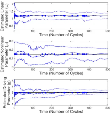
FIG. 5: (Color online) An example of values for all three parameters (˜ω, ˜µ, and ˜g) estimated simultaneously using SMC sampler with efficient measurements (η= 1.0, solid blue line) and 1001 sample points (other parameters are given in the text). Three standard deviation errors are indicated in each case with dotted lines, and the resampling points are indicated by circles along the solid black line.
value is achievable only in the long time limit and the actual error is likely to be significantly larger than this. In the examples given above, the SMC sampler produces parameter estimates with errors approaching this limit within a few hundred cycles. There is therefore a small but potentially significant benefit in using the SMC sam-pler method for one parameter estimation.
Moving from single to multiple parameter estimation presents a serious problem for grid-based methods. The number of points required scales exponentially in the number of dimensions to achieve the same accuracy. The error from a grid-based approach results from approxi-mating an integral of functions in D dimensions, where the error isO((Ngrid)(−1/D)). The error for an SMC sam-pler comes from approximating the integral directly (us-ing Monte-Carlo integration) and therefore isO(1/Ngrid) whatever value D takes [39]. (See reference [40] for proofs for the convergence of SMC and particle filter based methods). So, for D = 1, the two approaches offer similar scaling of error withNgrid, in higher dimen-sions, an SMC sampler will asymptotically outperform a grid-based method asNgrid tends to infinity. Of course, differences in constants of proportionality mean that a computational benefit from using the SMC sampler in a small number of dimensions (number of parameters) is not guaranteed. Estimating all three parameters in our example, at a level of accuracy equivalent to the one pa-rameter examples above, would require around ten mil-lion grid points, (300)3 = 9×10⁶. With SMC methods, this number is dramatically reduced.
Figure 5 shows an example of the simultaneous esti-mation of all three parameters using 1001 sample points. The values for ˜ω and ˜g still converge rapidly whilst ˜µ
takes longer to establish a stable estimate. When com-paring this with a grid based method, we note that the number of trajectories is larger than for the single pa-rameter case and the number of resampling events is also increased, approximately 20 in the case shown in Figure 5. This is equivalent to a run-time for approximately 10,000 trajectories on a fixed grid. Using the same as-sumptions as before, this would give errors limited by
σλ,grid >(λ/3 p
Ngrid)/ √
12'1.5%λ. The errors found using the SMC sampler described above are nearly an order of magnitude smaller than this limit for one of the three parameters (ω) and comparable for the remaining two parameters (µandg). There is an additional bene-fit, in that the sample points not only provide estimates of the parameter values, they also provide information regarding the correlations between the different parame-ters. For the example shown in Figure 5, the mean vector and the estimated covariance matrix (S) are given by
˜ ω ˜ µ ˜ g = 1.1981 0.1557 3.0874 S= 4.0308×10⁻³ −1.6449×10⁻⁶ 9.2270×10⁻⁶ −1.6449×10⁻⁶ 3.9795×10⁻⁴ −2.8254×10⁻⁶ 9.2270×10⁻⁶ −2.8254×10⁻⁶ 1.1586×10⁻² !
Note also that in Figure 5, the standard deviation of the linear parameter (˜ω) is larger than in Figure 2 and the convergence is slower than for the single parameter case. This is partly due to the larger uncertainty gener-ally in the three unknown parameters, and in part due to the slower convergence of the nonlinear parameter (˜µ). The coupling between the parameters, shown by the non-negligible correlations shown in the covariance matrix, means that uncertainty in the nonlinear parameter in-creases the standard deviation of the other two parame-ters.
The use of an SMC sampler to estimate the Hamil-tonian parameter values directly from the quantum tra-jectories is more efficient than an equivalent grid-based method but it still presents a computational challenge. Solving a single SME can be simplified using a stochastic integration method designed specifically for SMEs, like Rouchon’s method [58, 59], and using efficient numerical tools, like moving basis states [42, 43]. However, solv-ing many simultaneous SMEs to determine the evolution of the particle weights still requires significant compu-tational resources. The number of combinations of pa-rameter values explored using the SMC sampler is sig-nificantly less than that required by a conventional grid-based method, but each sample point explored requires the full trajectory to calculated, or recalculated after re-sampling. The number of SMEs required to be calculated can be said to berelativelysmall but it is still not a triv-ial exercise. In their favor, SMC methods are amenable to parallelization [16], since the evolution of SME and the recalculation of each trajectory after resampling are largely independent processes and can be distributed sim-ply across a number of processors. However, at present, it is more likely that this type of technique is more likely to be used for post-processing experimental data rather than as part of an on-line closed-loop control system.
VII. CONCLUSIONS
Continuous quantum measurements, and their
asso-ciated stochastic master equations (SMEs), provide a means to monitor the dynamical evolution of a quan-tum system and to provide an estimate of the underly-ing quantum state. In addition, the quantum trajecto-ries resulting from the integration of stochastic master equations contain useful information about the param-eters that govern the evolution of the system. Hybrid stochastic master equations provide a means to extract the information regarding these classical parameters. Hy-brid SMEs involve running many parallel SMEs, each one having a different value for the parameter (or parame-ters). The classical probabilities attached to the individ-ual SMEs and the associated parameter values can then be found by integrating a Kushner-Stratonovich equa-tion. This classical estimation process is numerically costly, and is even more so when estimates are required for multiple parameters. This paper has demonstrated how such estimates can be found using a technique taken from classical state estimation and nonlinear filtering, a Sequential Monte Carlo (SMC) sampler. The SMC sam-pler used in this paper has been demonstrated to allow the simultaneous estimation of three Hamiltonian param-eters, together with their statistical correlation and the associated quantum trajectories, in a computationally tractable form, with a relatively small number of can-didate parameter values and parallel SMEs.
Even with such methods, the computational task in solving the Hybrid SME is formidable, and is currently beyond the point where it could be used as part of a closed-loop quantum control system. At present, the strength of such techniques is in the ability to post-process experimental measurement data to verify the quantum states used in an experiment but also to provide an independent, in-situ means to check the parameters that govern their evolution.
Acknowledgments: JFR would like to thank the US
Army Research Laboratories (contract no. W911NF-16-2-0067). JFR would also like to thank Hendrik Ulbricht and Peter Barker for helpful and informative discussions.
[1] V. P. BelavkinReports on Mathematical Physics45, 353 (1999), and references contained therein.
[2] H. M. Wiseman, G. J. Milburn, ‘Quantum Measurement and Control’ (Cambridge University Press, Cambridge, 2010).
[3] K. Jacobs ‘Quantum Measurement Theory and Its Appli-cations’ (Cambridge University Press, Cambridge, 2014). [4] K. W. Murch, S. J. Weber, C. Macklin, I. Siddiqi,Nature
502, 211 (2013).
[5] S. J. Weber, A. Chantasri, J. Dressel, A. N. Jordan, K. W. Murch, I. Siddiqi, Nature511, 570 (2014).
[6] P. Six, P. Campagne-Ibarcq, L. Bretheau, B. Huard, P. Rouchon,54th IEEE Conference on Decision and Control Conference (CDC)(2015).
[7] P. Campagne-Ibarcq, P. Six, L. Bretheau, A. Sarlette, M. Mirrahimi, P. Rouchon, B. Huard,Physical Review X6, 011002 (2016).
[8] P. Smith, J. E. Reiner, L. A. Orozco, S. Kuhr, H. M. Wiseman,Physical Review Letters89, 133601 (2002). [9] S. Brakhane, W. Alt, T. Kampschulte, M.
Martinez-Dorantes, R. Reimann, S. Yoon, A. Widera, D. Meschede, Physical Review Letters109, 173601 (2012).
[10] Kuban A. Kubanek, M. Koch, C. Sames, A. Ourjoumt-sev, P. W. H. Pinkse, K. Murr, G. Rempe, Nature462, 898, (2009).
[11] D.J. Wilson, V. Sudhir, N. Piro, R. Schilling, A. H. Ghadimi, and T.J. Kippenberg,Nature,524, 325 (2015). [12] V. Sudhir, D.J. Wilson, R. Schilling, H. Sch¨utz, S. A.
Fedorov, A. H. Ghadimi, A. Nunnenkamp, and T.J. Kip-penberg,Physical Review X7, 011001 (2017).
[13] R. Vijay, C. Macklin, D.H. Slichter, S.J. Weber, K.W. Murch, R. Naik, A. N. Korotkov, I. Siddiqi,Nature490, 77 (2012).
[14] D. Rist`e,C.C. Bultink, K.W. Lehnert, and L. DiCarlo, Physical Review Letters109, 240502 (2012).
[15] J. F. Ralph, K. Jacobs, C. D. Hill,Physical Review A84, 052119 (2011).
[16] P. L. Green, S Maskell, Mechanical Systems and Signal Processing,93, 379396 (2017).
[17] I. L. Chuang, M. A. Nielsen,Journal Modern Optics44, 2455 (1997).
[18] J. Gambetta, H. M. Wiseman, Physical Review A 64, 042105 (2001).
[19] F. Verstraete, A. C. Doherty, H. Mabuchi,Physical Re-view A64, 032111 (2001).
[20] J. K. Stockton, J. M. Geremia, A. C. Doherty, H. Mabuchi,Physical Review A69, 032109 (2004).
[21] M. Tsang,Physcial Review Letters102, 250403 (2009). [22] M. Tsang,Physical Review A80, 033840 (2009). [23] M. Tsang,Physical Review A81, 013824 (2010). [24] M. Tsang, H.M. Wiseman, C.M. Caves,Physical Review
Letters106, 90401 (2011).
[25] A Negretti, K. Molmer,New Journal Physics15, 125002 (2013).
[26] D.W. Berry, M. Tsang, M.J.W. Hall, H.M. Wiseman, Physical Review X5, 031018 (2015).
[27] H. Bassa, S.K. Goyal, S.K. Choudhary, H. Uys, L. Di´osi, T. Konrad,Physical Review A92, 032102 (2015). [28] L. Cortez, A. Chantasri, L.P. Garc´ıa-Pintos, J. Dressel,
A.N. Jordan,Physical Review A95, 012314 (2017). [29] B.P. Abbott, R. Abbott, T.D. Abbott, et al., Physical
Review Letters116, 061102 (2016).
[30] F. Yang, A.J. Koll´ar, S.F. Taylor, R.W. Turner, B.L. Lev, Physical Review Applied7, 034026 (2017).
[31] N. Gordon, D. Salmond, A. F. Smith,IEE Proceedings F Radar Signal Processing,140, 107113 (1993).
[32] S. Blackman, ‘Multiple Target Tracking with Radar Ap-plications’ (Artech House, 1986)
[33] Y. Bar-Shalom, X.R. Li, T. Kirubarajan, ‘Estimation with Applications to Tracking and Navigation’ (Wiley & Sons, 2001).
[34] J. F. Ralph, ‘Target Tracking’ in ‘Encyclopedia of Aerospace Engineering’, Vol.5, Ch 251, eds. R. Blockley, W. Shyy (Wiley & Sons, 2010).
[35] H. M. Wiseman, A. Doherty,Physical Review Letters94, 070405 (2005).
[36] A. Doucet, N. De Freitas, and N. Gordon, Eds., ‘Sequen-tial Monte Carlo Methods in Practice’ (Springer, New York, 2001).
[37] O. Capp´e, S. J. Godsill, E. Moulines,Proceedings of the IEEE 95, 899 (2007).
[38] M. Arulampalam, S. Maskell, N. Gordon, T. Clapp, IEEE Transactions on Signal Processing 50, 241-254, (2002).
[39] W. H. Press, S. A. Teukolsky, W. T. Vetterling, B. P. Flannery, “Section 7.9.1 Importance Sampling” in “Nu-merical Recipes: The Art of Scientific Computing (3rd ed.)” (Cambridge University Press, New York, 2007). [40] D. Crisan, A. Doucet.IEEE Transactions on signal
pro-cessing50, 736-746 (2002).
[41] T. Hesterberg,Technometrics,37, 185-194 (1995). [42] R. Schack, T. A. Brun, I. C. Percival.Journal of Physics
A: Mathematical and General28, 5401 (1995).
[43] T. A. Brun, I. C. Percival, R. Schack,Journal of Physics. A: Mathematical and General292077 (1996).
[44] T. A. Brun, N. Gisin, P. F. O’Mahony, M. Rigo,Physics Letters A229267-272 (1997).
[45] S. Habib, K. Shizume, W. H. Zurek, Physical Review Letters80, 4361 (1998).
[46] T. Bhattacharya, S. Habib, K. Jacobs,Physical Review Letters854852 (2000).
[47] A. J. Scott, G. J. Milburn,Physical Review A63, 042101 (2001).
[48] T. Bhattacharya, S. Habib, K. Jacobs,Physical Review A7042103 (2003).
[49] M. J. Everitt, T. D. Clark, P. B. Stiffell, J. F. Ralph, A. R. Bulsara, C. J. Harland.New Journal of Physics 764 (2005).
[50] J. K. Eastman, J. J. Hope, A. R. R. Carvalho.Emergence of chaos controlled by quantum noise, arXiv:1604.03494 (2016).
[51] B. Pokharel, P. Duggins, M. Misplon, W. Lynn, K. Hall-man, D. Anderson, A. Kapulkin, A. K. Pattanayak, Dy-namical complexity in the quantum to classical transition, arXiv:1604.02743 (2016).
[52] J. F. Ralph, K. Jacobs, M. J. Everitt,Physical Review A
95, 012135 (2017).
[53] J. Gieseler, L. Novotny, R. Quidant,Nature Physics,9, 806 (2013).
[54] J. Gieseler, L. Novotny, C. Moritz, C. Dellago,New Jour-nal of Physics,17, 045011 (2015).
[55] M. Aikele, K. Bauer, W. Ficker, F. Naubauer, U. Prech-tel, J. Schalk, H. Seidel, Sensors and Actuators A 90, 161-167 (2001).
[56] R. M. C. Mestrom, R. H. B. Fey, H. Nijmeijer, IEEE/AMSE Transactions on Mechatronics14, 423-433 (2009).
[57] D. K. Agrawal, J. Woodhouse, A. A. Seshia,IEEE Trans. on Ultrasonics, Ferroelectrics and Frequency Control,60, 1646-1659 (2013).
[58] H. Amini, M. Mirrahimi, P. Rouchon,in Proc. 50th IEEE Conf. on Decision and Control, pp. 6242-6247 (2011). [59] P. Rouchon, J. F. Ralph,Physical Review A91, 012118
(2015).
[60] G.N. Milstein, ‘Numerical Integration of Stochastic Dif-ferential Equations’ (Springer, Berlin, 1995).
[61] J. F. Ralph, K. Jacobs, J. Coleman,Physical Review A