Computing approximate Fekete points by QR factorizations of Vandermonde matrices

(1)

Contents lists available atScienceDirect

Computers and Mathematics with Applications

journal homepage:www.elsevier.com/locate/camwa

Computing approximate Fekete points by QR factorizations of

Vandermonde matrices

I

Alvise Sommariva, Marco Vianello

∗

Department of Pure and Applied Mathematics, University of Padova, Italy

a r t i c l e i n f o Article history:

Received 20 March 2008

Received in revised form 28 October 2008 Accepted 8 November 2008

Keywords:

Approximate Fekete points Vandermonde matrices Maximum volume submatrices Greedy algorithm

QR factorization with column pivoting Algebraic quadrature

Polynomial interpolation Lebesgue constant Admissible mesh

a b s t r a c t

We propose a numerical method (implemented in Matlab) for computing approximate Fekete points on compact multivariate domains. It relies on the search of maximum volume submatrices of Vandermonde matrices computed on suitable discretization meshes, and uses a simple greedy algorithm based on QR factorization with column pivoting. The method gives also automatically an algebraic cubature formula, provided that the moments of the underlying polynomial basis are known. Numerical tests are presented for the interval and the square, which show that approximate Fekete points are well suited for polynomial interpolation and cubature.

1. Introduction

LetΩ

⊂

_Rd_{be a compact subset (or lower dimensional manifold). Given a polynomial basis for}_Πd

n

(

Ω

)

(the subspace of d-variate polynomials of total degree

≤

nrestricted toΩ), say

span

(

pj)1≤j≤N

=

Πnd

(

Ω

),

N

=

N

(

n

)

:=

dim

(

Π d

n

(

Ω

)),

(1)

and a sufficiently large and dense discretization ofΩ

X

= {

xi

} ⊂

Ω

,

1

≤

i

≤

M

,

M

>

N

,

(2)

we can construct the rectangular Vandermonde matrix

V

=

Vn(x1

, . . . ,

xM)

=

(vij)

:=

(

pj(xi))

∈

RM×N

.

(3)

A quadrature formula of algebraic degree of exactness nfor a given measure

µ

onΩ can be obtained by solving the underdetermined linear system of the quadrature weights

M

X

i=1

wi

pj(xi)

=

Z

Ω pj(x

)

d

µ,

1

≤

j

≤

N (4)

I_{Work supported by the ‘‘ex-60%’’ funds of the University of Padova, and by the INdAM GNCS. This work is published despite the drastic reduction} of public funding for universities and research pursued by the Italian government (see the article ‘‘Cut-throat savings’’, Nature 455, October 2008, http://www.nature.com/nature/journal/v455/n7215/full/455835b.html).

∗_{Corresponding author.}

E-mail address:[email protected](M. Vianello).

(2)

that is in matrix form Vt

w

=

m

,

m

= {

mj

} =

Z

Ω pj(x

)

d

µ

,

1

≤

j

≤

N

,

(5)

provided that the ‘‘moments’’

{

mj

}

are explicitly known or computable (cf., e.g., [1,2] for the computation of polynomial

moments over nonstandard domains). We observe that in the numerical literature there is no universal agreement on the terminology on Vandermonde matrices, oftenVt(in our notation) is called the Vandermonde matrix; see, e.g., [3].

The solution of such a system by a standard SVD approach (cf. [3,4]) would then give in general a vector ofMnonzero weights, and thus a quadrature formula which uses all the original discretization points; this has been confirmed by all our numerical experiments, where zero or nearly zero weights (compared to the others) do not appear, indeed all the weights have the same size. On the contrary, ifVt_{has full rank, its solution by the standard Matlab backslash ‘‘}

_\

_{’’ solver for linear}

systems (cf. [5]) gives onlyNnonzero weights, and thus also an automatic selection of the relevantNquadrature nodes and weights. In a Matlab-like notation we can write:

Algorithm 1 (Approximate Fekete points, Full Rank Vt).

• w

=

Vt

\

m

;

ind

=

find

(w

6=

0

)

;

•

X∗

=

X

(

ind

)

;

w

∗

=

w(

ind

)

;

V∗

=

V

(

ind

,

:

)

;

where ind

=

(

i1

, . . . ,

iN), that is we get the two arrays of lengthN

X∗

= {

xi1

, . . . ,

xiN

}

,

w

∗

= {

wi

1

, . . . , wi

N

}

,

(6)

which generate the quadrature formula

Z

Ω f

(

x

)

d

µ

≈

N

X

k=1

wi

kf

(

xik

),

f

∈

C

(

Ω

).

(7)

Moreover, we also extract a nonsingular Vandermonde submatrixV∗(corresponding to the selected points), which can be useful for polynomial interpolation. When rank

(

Vt

) <

N,Algorithm 1fails to extract the correct number of points. This means that polynomial interpolation at that degree is not possible by the extraction procedure (a remedy for this situation is discussed in Section3). Computing quadrature weights from moments via square Vandermonde matrices is a well-known and developed approach in the one-dimensional case (see, e.g., [6]), whereas the general and multidimensional extraction procedures just sketched (based on rectangular Vandermonde matrices) seems in some respect new.

Our numerical experiments in the interval and in the square show that, when suitable polynomial bases are used, this approach gives a good (stable and convergent) quadrature formula, and in addition the extracted quadrature nodes are good polynomial interpolation points (slow growth of the Lebesgue constant).

This is essentially due to the implementation of the Matlab backslash command for underdetermined linear systems, which is based on the QR factorization algorithm with column pivoting, firstly proposed by Businger and Golub in 1965 (cf. [7]). The backslash command for rectangular matrices uses the LAPACK routine DGEQP3, see the ‘‘mldivide’’ command page in [5,8].

The result is that such points are approximate Fekete points, that is points computed by ‘‘trying to maximize’’ the Vandermonde determinant absolute value, as we shall discuss in the next sections. Our work is mainly of computational kind, for a deep discussion about the theoretical issues of the present approach in the one-dimensional case we refer the reader to the work in progress [9].

2. Approximate Fekete points in the interval

In order to show the potentialities of the method, we present inTable 1below some relevant parameters concerning quadrature and interpolation in the one-dimensional case,Ω

= [−

1

,

1

]

and d

µ

=

dx. The nodes are extracted from a uniform grid of 5000 points (seeRemark 1) at a sequence of degrees,n

=

10

,

20

, . . . ,

60, with three different polynomial bases (the monomial, the Legendre and the Chebyshev basis). The parameters (given with two or three significant figures) are the spectral condition number of the transpose rectangular Vandermonde matrix, the euclidean norm of the weights’ system residual (say

k

res

(w)

k

₂

= k

m

−

Vt

_w

_k

2), the sum of the weights’ absolute values (a measure of the quadrature

stability, cf. [10]), the Lebesgue constantΛn(a measure of the interpolation stability, cf. [11]: such a quantity is evaluated

numerically on a very large set of control points). Concerning quadrature, the required moments are known analytically, in particular by orthogonality the integrals of the Legendre basis polynomials are all vanishing except at degree zero (cf., e.g., [12] for the Chebyshev basis).

We can see that both the orthogonal bases give very good results, the best in terms of Lebesgue constant being obtained with the Chebyshev basis. On the contrary, the monomial basis suffers from ill-conditioning of Vandermonde matrices, which at higher degrees become even rank-deficient, i.e. rank

(

Vt

_{) <}

_N_{, so that as observed above}_{Algorithm 1}_{fails to}

(3)

Table 1

Relevant parameters for the extracted points,Ω= [−1,1](where (+) means that the weights are all positive, and∗means thatAlgorithm 1fails to extract N=n+1 points due to rank-deficiency).

Basis n=10 n=20 n=30 n=40 n=50 n=60

Mon cond(Vt₎ _3.1E₊₀₃ _1.8E₊₀₇ _1.1E₊₁₁ _6.7E₊₁₄ _1.7E₊₁₆ _3.6E₊₁₆

kres(w)k2 5.5E−16 1.4E−15 5.1E−12 2.8E−10 3.1E−10 2.0E−10 P_|_w

ik| 2.00(+) 2.00(+) 5.31 5.47 93.6 56.7

Λn 5.33 5.06 ∗(30pts) ∗(30pts) ∗(32pts) ∗(35pts)

Leg cond(Vt₎ _4.6E₊₀₀ _6.4E₊₀₀ _7.8E₊₀₀ _9.0E₊₀₀ _1.0E₊₀₁ _1.1E₊₀₁

kres(w)k2 6.6E−16 7.0E−16 1.1E−15 2.3E−15 1.4E−15 2.0E−15 P_|_w

ik| 2.00(+) 2.00(+) 2.01 2.05 2.00(+) 2.00(+)

Λn 2.74 5.94 7.11 9.59 10.9 12.4

Cheb cond(Vt₎ _3.7E₊₀₀ _5.0E₊₀₀ _6.0E₊₀₀ _6.7E₊₀₀ _7.1E₊₀₀ _7.5E₊₀₀

kres(w)k2 1.2E−15 1.4E−15 1.6E−15 1.8E−15 1.9E−15 2.1E−15 P

|wik| 2.00(+) 2.00(+) 2.00(+) 2.00(+) 2.00(+) 2.00(+)

Λn 2.27 2.79 3.13 3.40 3.58 3.80

procedure. Nevertheless, a quadrature formula can be constructed with a number of points (in parentheses) that is less than the dimension of the polynomial space of ‘‘exactness’’, and which still gives acceptable results (see alsoTable 5below). Observe that we could have computed the Lebesgue constant also in the cases of failure using the available nodes, but we have avoided this since it makes sense only in one dimension (where any natural number can be the dimension of a polynomial subspace).

The good behavior of the points selected byAlgorithm 1, for algebraic quadrature and for polynomial interpolation (at least when suitable polynomial bases are used), is directly related with the features of the Matlab ‘‘backslash’’ linear solver. In fact, in the case of underdetermined systems, such a solver performs a QR factorization with column pivoting of the matrix (cf. [4,5,7]). In practice, this corresponds to a special QR factorization of the transpose Vandermonde submatrixVt

∗

∈

RN

×N_,

that is

(

VtP

)(

:

,

1

:

N

)

=

V_∗t

=

QR

,

(8)

whereQ is orthogonal,Rupper triangular with

|

r11

| ≥ |

r22

| ≥ · · · ≥ |

rNN

|

, andPa permutation matrix. More precisely,

since inside a QR process with stepwise selection of the columns, we can see the diagonal element ofRproduced at a given step as a function of the matrix columns involved so far,

rkk

=

rkk(γ1

, . . . , γk),

0

≤

k

≤

N

,

γj

∈

col1

(

Vt

), . . . ,

colM(Vt

)

⊂

RN

,

(9) it can be shown that the QR algorithm with column pivoting acts in such a way to maximizerkkas a function of the vector

variable

γk

(the vector variables

γ

1

, . . . , γk

−1having been fixed by the previous steps); cf., e.g., [3, Section 2.7.3]. In other

words, since

|

det

(

V_∗t

)

| = |

det

(

V∗

)

| =

N

Y

k=1

|

rkk

|

,

(10)

all the process can be re-interpreted as a heuristic optimization of the extracted Vandermonde determinant (as a function ofNof theMoriginal discretization points), based on sequential componentwise maximization of the factors.

An equivalent but more ‘‘geometric’’ interpretation of Algorithm 1 is that related with the notion of volume of submatrices. Indeed, it can be shown that the QR factorization(8) (the core of the algorithm) is an implementation of the standard ‘‘greedy’’ approximation algorithm for selectingNcolumns with maximal associated volume, which can be sketched as follows:

Algorithm greedy (Max Volume Submatrix of A

∈

_RN×M_{, M}

_>

_N_).

•

ind

= [ ] ;

•

fork

=

1

, . . . ,

N

– ‘‘select the largest norm columncolik

(

A

)

’’; ind

= [

ind

,

ik

]

;

– ‘‘remove from every column ofAits orthogonal projection ontocolik;

end;

see, e.g., [9,13] and the references therein. It is worth stressing that(8)acts only on the matrix and thus the mere selection of the points inAlgorithm 1could be done with any right-hand side in the system (i.e., it is independent of the specific quadrature problem).

Observe that such a discrete nonlinear optimization problem is known to be NP-Hard (cf. [13]), and thus heuristic/stochastic methods are mandatory. The strength ofAlgorithm 1is that it gives good results in practice, by using only basic optimized tools of numerical linear algebra. We stress that the use of the commercial package Matlab for this

(4)

Table 2

Absolute value of the Vandermonde determinants (in the Chebyshev basis) for different families of points,Ω= [−1,1];∗indicates algorithm failure due to rank-deficiency.

Points n=10 n=20 n=30 n=40 n=50 n=60

Eq spaced 8.4E+02 2.0E+03 6.7E−01 1.3E−08 1.1E−20 2.2E−37

Approx Fek

Basis mon 9.6E+03 7.3E+10 ∗ ∗ ∗ ∗

Basis Leg 2.4E+04 6.5E+10 1.7E+18 2.0E+26 1.0E+35 2.2E+44

Basis Cheb 3.1E+04 1.5E+11 8.4E+18 2.3E+27 2.0E+36 5.6E+45

True Fek 3.1E+04 1.5E+11 8.6E+18 2.5E+27 2.4E+36 6.2E+45

ChebLob 2.8E+04 1.3E+11 6.8E+18 2.0E+27 1.8E+36 4.5E+45

GaussCheb 1.7E+04 7.5E+10 4.0E+18 1.1E+27 1.0E+36 2.7E+45

problem is user-friendly and practical due to its wide diffusion, but the implementation can be done by other open-source libraries and computing systems, e.g. using directly LAPACK subroutines; cf. [8,14] and the references therein.

Points that maximize the Vandermonde volume in the continuum, the so-called Fekete (or extremal) points, are important in polynomial interpolation (see, e.g., [15,16]). This stems directly from the representation of the Lagrange cardinal polynomials for a given unisolvent set at degreen, say

{

ξ

₁

, . . . , ξN

}

, as the ratio of two Vandermonde determinants

L_ξ_i

(

x

)

=

det

(

Vn(ξ1

, . . . , ξi

−1

,

x

, ξi

+1

, . . . , ξN))

det

(

Vn(ξ1

, . . . , ξi

−1

, ξi

+1

, . . . , ξN

))

,

L_ξ_i

(ξk)

=

δik,

(11)

(cf.(3)for the definition ofVn), from which it is clear that at a subset ofΩ which maximizes the absolute value of the

Vandermonde determinant, sayFn

= {

φ

1

, . . . , φN

}

, we have that the Lebesgue constant (the norm of the interpolation

operator) is bounded byN

k

L_φ_i

k

∞

=

1

,

1

≤

i

≤

N

H⇒

Λn

:=

max x∈Ω N

X

i=1

|

L_φ_i

(

x

)

| ≤

N

.

(12) Such a rough estimate already shows that Fekete points are good interpolation points. Moreover, they can be also near-optimal interpolation points, as it happens in the one-dimensional case, where they are known to be the Gauss–Lobatto points by a classical result of Fejér and to have a Lebesgue constant growing likeO

(

logn

)

(cf. [17]). Much less is known in higher dimension, see [18] and the references therein.

The numerical computation of high-degree Fekete points on a givend-dimensional compact subset is a hard large-scale problem, since it corresponds to the optimization of a nonlinear function with 2Nvariables (recall thatN

∼

nd

_/

_d

_!

_{). Indeed}

even in important two-dimensional instances, like the triangle which is relevant for the application to spectral element methods for PDEs, Fekete points have been computed only up to relatively small degrees; cf., e.g., [19–21] and the references therein. A big effort has been made to compute Fekete (or extremal) points on the sphere, in view of their importance in applications, by methods that need large-scale computational resources, cf. [22] and the references therein.

On the other hand, also the computation of good points for algebraic quadrature over d-dimensional compact subsets, especially for the so-called minimal quadrature formulas, is a substantially open problem with several important applications, whose direct numerical solution again involves large-scale nonlinear problems; cf., e.g., [23,24] and the references therein.

Our numerical experiments have shown that Algorithm 1 gives a reasonable compromise between quality of the quadrature/interpolation points, and computational cost. As sketched above, the method is related with the maximization of Vandermonde volumes, and thus we can call the produced points ‘‘approximate Fekete points’’. The following tables give more evidence in this direction, by comparing the Vandermonde volume (Table 2) and the Lebesgue constant (Table 3) of the one-dimensional Fekete points with that of equally spaced points, of the three families of approximate Fekete points of

Table 1, and of the Gauss–Chebyshev and Chebyshev–Lobatto points which are known to be excellent interpolation points (the Vandermonde matrix is computed in the Chebyshev basis in all instances).

InTable 4, we report the distance in

k · k

∞of different arrays of approximate Fekete points from the true Fekete points (ordered arrays). The superiority of the orthogonal bases is confirmed also in terms of these parameters: in particular, the approximate Fekete points obtained by the Chebyshev basis are in all respects the closest to the true Fekete points.

It is worth stressing the fact that, at least in the complex case (polynomial interpolation in_C), there is a sound theoretical basis for the connection of our approximate discrete Fekete points with the continuum Fekete points, as is made clear by the following key result (cf. [9]) which applies in particular to the case of the interval.

Theorem 1 (Bos and Levenberg, [9]).Suppose thatΩ

⊂

_Cis a continuum (i.e. compact and connected, not a single point). Suppose further that Xn

⊂

Ω, n

=

1

,

2

, . . .

, are discrete subsets of Ωsuch that for all x

∈

Ω

min

y∈Xn

|

x

−

y

| ≤

φ(

n

),

where lim

n→∞n

2

_φ(

_n

₎

₌

₀

_.

₍₁₃₎

(5)

Table 3

Comparison of the Lebesgue constants for different families of points,Ω= [−1,1];∗indicates algorithm failure due to rank-deficiency.

Points n=10 n=20 n=30 n=40 n=50 n=60

Eq spaced 29.9 1.10E+04 6.60E+06 4.05E+08 7.34E+09 1.24E+10

Approx Fek Basis mon 5.33 5.06 ∗ ∗ ∗ ∗ Basis Leg 2.74 5.94 7.11 8.59 10.9 12.4 Basis Cheb 2.27 2.79 3.13 3.40 3.58 3.80 True Fek 2.18 2.61 2.86 3.04 3.18 3.30 ChebLob 2.42 2.87 3.13 3.31 3.45 3.57 GaussCheb 2.49 2.90 3.15 3.33 3.47 3.58 Table 4

Distances ink·k∞of the approximate from the true Fekete points’ array,Ω= [−1,1](ordered arrays);∗indicates algorithm failure due to rank-deficiency.

Points n=10 n=20 n=30 n=40 n=50 n=60

Approx Fek

Basis mon 1.3E−01 4.3E−02 ∗ ∗ ∗ ∗

Basis Leg 5.9E−02 6.1E−02 5.8E−02 4.2E−02 3.0E−02 2.4E−02

Basis Cheb 9.1E−03 6.6E−03 6.1E−03 4.8E−03 4.0E−03 3.6E−03

Table 5

Quadrature and interpolation errors for the Runge function;∗indicates algorithm failure due to rank-deficiency.

Points n=10 n=20 n=30 n=40 n=50 n=60

Approx Fek

Basis mon Quadr 1.9E−02 2.0E−04 3.5E−04 8.2E−05 4.9E−04 4.8E−04

Interp 1.9E+00 1.5E−01 ∗ ∗ ∗ ∗

Basis Leg Quadr 2.7E−03 1.6E−03 3.9E−05 6.8E−06 3.8E−07 6.7E−08

Interp 1.6E+00 1.8E−01 1.5E−02 1.3E−03 9.8E−05 1.1E−05

Basis Cheb Quadr 9.6E−03 6.7E−05 6.8E−07 1.2E−07 2.1E−09 6.8E−10

Interp 1.7E+00 1.3E−01 1.1E−02 9.6E−04 8.1E−05 6.8E−06

True Fek Quadr 8.9E−03 6.2E−05 4.4E−07 3.1E−09 2.2E−11 1.6E−13

Interp 1.6E+00 1.3E−01 1.1E−02 9.5E−04 7.8E−05 6.7E−06 Then, independently of the bases used, Algorithm1will generate sets of approximate Fekete points that have the same asymptotic distribution (see [25]) as do the true Fekete points. Specifically, the positive measure of total mass1obtained by assigning to every point a mass of 1

/(

n

+

1

)

converges weakly to the equilibrium measure forΩ.

Remark 1. It is worth recalling that many other families of points have the same asymptotic distribution in the case of the interval,Ω

= [−

1

,

1

]

, e.g. the zeros of Jacobi polynomials. The property that the approximate Fekete points array converges in

k · k

∞to the true Fekete points is stronger than the weak-* convergence given byTheorem 1, and has only some numerical evidence such as that given inTable 4.

Notice that the numberM

=

5000 of discretization points used in the numerical experiments on the interval, is consistent with the assumptions ofTheorem 1up to the highest degree (n2

₌

₆₀2

₌

_{3600). On the other hand, it is also consistent}

with the spacing of the true Fekete points (the minimum of pairwise distances) in complex compact sets of unit capacity, which is bounded from below by 2

/(

en2

₎

_for_n

_≥

_{4, cf. [}₂₅_{]. The number of extraction points could be tuned to the degree,}

namely one could compute approximate Fekete points in

[−

1

,

1

]

at degreenfrom a uniform grid with stepsize 1

/(

en2

₎

_{. This}

has been tried in our numerical experiments, obtaining results close to those displayed inTables 1–5.

We conclude this section by showing a numerical test (Table 5), where the quadrature and interpolation errors of the Runge functionf

(

x

)

=

1

/(

1

+

16x2

₎

_{at approximate Fekete points of}_{Table 1}_{are compared with those at the true Fekete}

points. The interpolating polynomial has been computed by solving the corresponding square Vandermonde system with standard Gaussian elimination (again, the ‘‘

\

’’ command in Matlab).

As expected, the points obtained via the Chebyshev–Vandermonde matrix are excellent quadrature/interpolation points. Notice that the points corresponding to the monomial basis even in the presence of severe ill-conditioning and rank-deficiency are able to give acceptable quadrature results, but with an observed error stalling aroundO

(

10−4

₎

_.

3. Iterative refinement

The approximate Fekete points computed byAlgorithm 1depend on the polynomial basis adopted, as is clear from the previous tables (even though, in the one-dimensional case, all these points should have asymptotically the same distribution as do the true Fekete points, in view ofTheorem 1).

(6)

Using ‘‘wrong’’ bases, especially for the interpolation problem, leads to ‘‘bad’’ sets of points, due to the extreme ill-conditioning of the Vandermonde matrices, or even to computational failure since such matrices can become rank-deficient. As it is well known in the one-dimensional case, the problem of ill-conditioning is typical of the monomial basis. We recall, for example, that in view of the results of [26], the spectral conditioning ofVtfor the monomial basis whenM

N

=

n

+

1 is expected to be close to the square root of the conditioning of the Hilbert matrix of orderN. The ill-conditioning can be attenuated or even eliminated by resorting to bases of orthogonal polynomials; cf., e.g., [3,27] and the references therein. This behavior is also evident inTable 1.

The following iterative refinement algorithm, based on successive changes of basis by QR factorizations of the (nontranspose) Vandermonde matrices (with Q rectangular orthogonal and R square upper triangular), tries to give a computational solution to the problem of the basis choice. This will be particularly relevant in dimension greater than 1, where bases of orthogonal polynomials are not known explicitly for general domains.

Algorithm 2 (Approximate Fekete Points by Iterative Refinement).

•

V0

=

V

;

P0

=

I

;

•

fork

=

0

, . . . ,

s

−

1 Vk

=

QkRk

;

Uk

=

inv

(

Rk)

;

Vk+1

=

VkUk

;

Pk+1

=

PkUk

;

end;

• µ

=

Pt sm

;

w

=

Vst

\

µ

;

ind

=

find

(w

6=

0

)

;

•

X∗

=

X

(

ind

)

;

w

∗

=

w(

ind

)

;

V∗

=

Vs(ind

,

:

)

;

We stress that multiplication byUkcorresponds to a change of basis in the Vandermonde matrix, in such a way that

starting from a polynomial basisp

=

(

p1

, . . . ,

pN)the final basis will beq(s)

=

(

q( s) 1

, . . . ,

q

(s)

N

)

=

pPs(the column vector of

moments must then be transformed into

µ

=

Pt sm).

IfV0

=

Vis not severely ill-conditioned, thenQ0is numerically orthogonal andV1

=

V0U0is close toQ0, that is the

basisq(1)

₌

_pP

1is (numerically) orthogonal with respect to a discrete inner product defined on the originalMdiscretization

points ofΩ

h

q(_j1)

,

q(_h1)

i :=

M

X

i=1 q_j(1)

(

xi)q_h(1)

(

xi)

=

(

V₁tV1

)jh

≈

(

Q0tQ0

)jh

=

0

,

j

6=

h

.

(14)

IfV0is severely ill-conditioned, thenQ0might be far from orthogonality, and in addition since alsoR0is ill-conditioned

thenV1

=

V0U0is not close toQ0. Nevertheless,Q0and evenV1are much better conditioned thanV0. WhenV0is numerically

full rank (cf. [28]), the second iteration givesQ1orthogonal up to machine precision (the rule of ‘‘twice is enough’’, cf. [28]),

andV2near-orthogonal or at least sufficiently well conditioned to apply successfullyAlgorithm 1. In practice, however, often

one iteration is sufficient.

Algorithm 2can work even whenV₀tis numerically rank-deficient (see the asterisks inTable 6foriter

=

0), since after some iterations we can get full rank and then another one or two iterations usually suffice as just described. The functional interpretation ofAlgorithm 2is that the basisq(k)

₌

_pP

kapproaches a sort of discrete orthogonality at the originalM

discretization points ofΩ.

InTables 6–8, the effect of iterative refinement is shown on the three families of points ofTable 1. Observe that 1–2 iterations give a substantial improvement of the quality of the extracted points, for both the monomial and the Legendre basis (beyond, a stalling of the stability parameters is observed). On the contrary, a slight worsening appears with the Chebyshev basis concerning the Lebesgue constant (but only on the second significant figure), since this is already an excellent basis for the extraction process, whereas the iterative refinement tends to produce the same discrete orthonormal basis (triangular like the starting bases). Indeed, unless the initial conditioning is too severe as with the monomial basis at high degrees, we can see that the final Lebesgue constants are (nearly) the same for all the bases, and increase very slowly (compare again with the true Fekete points).

In order to appreciate the quality of the approximate Fekete points obtained after the iterative refinement process, in

Table 9we compare again the quadrature and interpolation errors on the Runge test function. The interpolation matrix isV∗

=

Vs(ind

,

:

)

=

V

(

ind

,

:

)

Ps, cf.Algorithm 2. The performance is now very good also with the Legendre basis at all

degrees, and with the monomial basis at low degrees. With the monomial basis at higher degrees, where we have a severe ill-conditioning of the original Vandermonde matrix (which entails also a severe ill-conditioning of the transformation matrixP_s), we can observe an error stalling/worsening as inTable 5(no refinement), but remaining in any case 2–3 orders of magnitude below the unrefined case.

4. Towards multivariate Fekete points

The computation of approximate Fekete points in multivariate instances is a challenging problem. In principle,

Algorithms 1and2can be applied in any compact domain, as soon as a suitable basis and initial set of points have been chosen. So, the basic questions are: given a multidimensional compact domain, which could be a reasonable distribution of points? and which could be a reasonable basis to work with? The answers depend strongly on the geometry of the domain.

(7)

Table 6

Iterative refinement of the approximate Fekete points extracted with the monomial basis,Ω= [−1,1];∗indicates algorithm failure due to rank-deficiency.

iter n=10 n=20 n=30 n=40 n=50 n=60

cond(Vt₎ ₀ _3.1E₊₀₃ _1.8E₊₀₇ _1.1E₊₁₁ _6.7E₊₁₄ _1.7E₊₁₆ _3.6E₊₁₆

1 1.0E+00 1.0E+00 1.0E+00 1.0E+00 1.1E+09 3.3E+12

2 1.0E+00 1.0E+00 1.0E+00 1.0E+00 1.0E+00 1.0E+00

3 1.0E+00 1.0E+00 1.0E+00 1.0E+00 1.0E+00 1.0E+00

kres(w)k2 0 5.5E−16 1.4E−15 5.1E−12 2.8E−10 3.1E−10 2.0E−10

1 5.9E−16 1.1E−17 2.2E−17 2.3E−17 2.5E−14 7.3E−13

2 7.5E−16 1.9E−17 2.1E−17 2.4E−17 2.9E−17 4.7E−17

3 2.1E−16 4.7E−18 2.0E−17 1.7E−17 3.5E−17 3.5E−17

P_|_w ik| 0 2.00(+) 2.00(+) 5.31 5.47 93.6 56.7 1 2.00(+) 2.00(+) 2.00(+) 2.00(+) 24.0 22.0 2 2.00(+) 2.00(+) 2.00(+) 2.00(+) 2.17 2.23 3 2.00(+) 2.00(+) 2.00(+) 2.00(+) 2.13 2.34 Λn 0 5.33 5.06 ∗ ∗ ∗ ∗ 1 2.38 2.93 3.29 3.54 7.56 10.2 2 2.38 2.93 3.29 3.54 5.49 9.69 3 2.38 2.93 3.29 3.54 5.49 9.69 True FekΛn 2.18 2.61 2.86 3.04 3.18 3.30 Table 7

Iterative refinement of the approximate Fekete points extracted with the Legendre basis,Ω= [−1,1].

iter n=10 n=20 n=30 n=40 n=50 n=60

cond(Vt₎ ₀ _4.6E₊₀₀ _6.4E₊₀₀ _7.8E₊₀₀ _9.0E₊₀₀ _1.0E₊₀₁ _1.1E₊₀₁

1 1.0E+00 1.0E+00 1.0E+00 1.0E+00 1.0E+00 1.0E+00

2 1.0E+00 1.0E+00 1.0E+00 1.0E+00 1.0E+00 1.0E+00

kres(w)k2 0 6.6E−16 7.0E−16 1.1E−15 2.3E−15 1.4E−15 2.0E−15

1 1.4E−17 1.7E−17 2.3E−17 2.8E−17 2.8E−17 3.6E−17

2 1.4E−17 2.0E−17 2.1E−17 2.8E−17 2.2E−17 4.2E−17

P_|_w ik| 0 2.00(+) 2.00(+) 2.01 2.05 2.00(+) 2.00(+) 1 2.00(+) 2.00(+) 2.00(+) 2.00(+) 2.00(+) 2.00(+) 2 2.00(+) 2.00(+) 2.00(+) 2.00(+) 2.00(+) 2.00(+) Λn 0 2.74 5.94 7.11 9.59 10.9 12.4 1 2.38 2.93 3.29 3.54 3.72 3.90 2 2.38 2.93 3.29 3.54 3.72 3.90 True FekΛn 2.18 2.61 2.86 3.04 3.18 3.30 Table 8

Iterative refinement of the approximate Fekete points extracted with the Chebyshev basis,Ω= [−1,1].

iter n=10 n=20 n=30 n=40 n=50 n=60

cond(Vt₎ ₀ _3.7E₊₀₀ _5.0E₊₀₀ _6.0E₊₀₀ _6.7E₊₀₀ _7.1E₊₀₀ _7.5E₊₀₀

1 1.0E+00 1.0E+00 1.0E+00 1.0E+00 1.0E+00 1.0E+00

2 1.0E+00 1.0E+00 1.0E+00 1.0E+00 1.0E+00 1.0E+00

kres(w)k2 0 1.2E−15 1.4E−15 1.6E−15 1.8E−15 1.9E−15 2.1E−15

1 1.0E−17 2.0E−17 2.0E−17 2.4E−17 2.8E−17 2.7E−17

2 7.0E−18 1.8E−17 2.2E−17 2.7E−17 2.3E−17 2.9E−17

P |wik| 0 2.00(+) 2.00(+) 2.00(+) 2.00(+) 2.00(+) 2.00(+) 1 2.00(+) 2.00(+) 2.00(+) 2.00(+) 2.00(+) 2.00(+) 2 2.00(+) 2.00(+) 2.00(+) 2.00(+) 2.00(+) 2.00(+) Λn 0 2.27 2.79 3.13 3.40 3.58 3.80 1 2.38 2.93 3.29 3.54 3.72 3.90 2 2.38 2.93 3.29 3.54 3.72 3.90 True FekΛn 2.18 2.61 2.86 3.04 3.18 3.30

Concerning the basis, the computational experience and the univariate theory (cf. [3,27]) show that a better conditioning is obtained using orthogonal bases (when available, cf. [29] about multivariate orthogonal polynomials), and that

Algorithm 2can improve substantially bases that are not ‘‘too bad’’, depending on the level of conditioning of the initial Vandermonde matrix.

Concerning the initial set of points, in the univariate caseTheorem 1gives a clear guideline, and it is worth recalling that the (continuum) Fekete points are known to be asymptotically nearly equally spaced with respect to the arccos metric. In multivariate instances, much less is known about the distribution of Fekete points. Some results have been recently obtained on the spacing of Fekete points in important standard geometries, like the sphere, the ball and the simplex, which can be

(8)

Table 9

Absolute quadrature and interpolation errors for the Runge function at the approximate Fekete points extracted after 2 refinement iterations (comparison with the true Fekete points).

Points n=10 n=20 n=30 n=40 n=50 n=60

Approx Fek

Basis mon Quadr 1.2E−02 1.1E−04 1.9E−06 4.7E−08 5.3E−07 6.8E−07

Interp 1.7E+00 1.3E−01 1.1E−02 9.3E−04 3.2E−04 2.8E−04

Basis Leg Quadr 1.2E−02 1.1E−04 1.9E−06 2.3E−09 8.2E−10 2.5E−10

Interp 1.7E+00 1.3E−01 1.1E−02 9.3E−04 7.8E−05 6.5E−06

Basis Cheb Quadr 1.2E−02 1.1E−04 1.9E−06 2.3E−09 8.2E−10 2.5E−10

Interp 1.7E+00 1.3E−01 1.1E−02 9.3E−04 7.8E−05 6.5E−06

True Fek Quadr 8.9E−03 6.2E−05 4.4E−07 3.1E−09 2.2E−11 1.6E−13

Interp 1.6E+00 1.3E−01 1.1E−02 9.5E−04 7.8E−05 6.7E−06

summarized as c1

n

≤

min

{

dist

(

a

,

b

),

b

∈

Fn,b

6=

a

} ≤

c2

n

,

∀

a

∈

Fn, (15)

whereFnis a set of Fekete points for the domain,c1

,

c2are positive constants and ‘‘dist’’ is the Dubiner (sphere, ball) or

the Baran (simplex) metric (which are generalizations of the arccos metric); see [18,30,31] and the references therein. The lower bound holds for the former withc1

=

π/

2 in any compact set, by a general result of Dubiner [15,31].

These results give further support to the conjecture (Bos [32], see also [33]) that ‘‘near-optimal’’ multivariate interpolation points in general compact domains, and in particular Fekete points, are asymptotically nearly equally spaced with respect to the Dubiner metric. We recall that the Dubiner metric on a compact subsetΩ

⊂

_Rd_{has the following definition}

dist_D

(

a

,

b

)

:=

sup

_|

arccos

(

p

(

b

))

−

arccos

(

p

(

a

))

|

deg

(

p

)

,

k

p

k

Ω

≤

1

,

deg

(

p

)

≥

1

,

(16)

for every pair of pointsa

,

b

∈

Ω, cf. [15].

Such a distance is known in explicit form only for very few domains, namely for the square

distD

(

a

,

b

)

=

max

{|

arccos

(

a1

)

−

arccos

(

b1

)

|

,

|

arccos

(

a2

)

−

arccos

(

b2

)

|}

,

(17)

a

=

(

a1

,

a2

),

b

=

(

b1

,

b2

)

∈

Ω

= [−

1

,

1

]

2, for the sphere where it turns out to be simply the geodesic distance, and for the

disk where it is obtained by projection on a corresponding hemisphere distD

(

a

,

b

)

=

arccos

a1a2

+

b1b2

+

q

1

−

a2₁

−

b2₁

q

1

−

a2₂

−

b2₂

,

(18) a

,

b

∈

Ω

= {

z

=

(

z1

,

z2

)

:

z12

+

z22

≤

1

}

, with natural generalizations in higher dimension to hypercubes, hyperspheres and

balls (cf. [18,30,31]).

4.1. Approximate Fekete points in the square

Consider now, as a guideline, the case of the squareΩ

= [−

1

,

1

]

2_{, with d}

_µ

₌

_d_x_{for the quadrature problem. It is worth}

recalling that Fekete points are known in this case only for tensor-product polynomial spaces [34], whereas here we are interested in total degree polynomial spaces.

We can proceed by the following approach, which is still of heuristic nature. Assume that at degreenthere are (at least two) Fekete points in a euclidean neighborhood of the boundary with radiusO

(

1

/

n

)

, a fact that even though not rigorously proved till now, is verified numerically (indeed, Fekete points cluster at the boundary). Then from the spacing inequality

(15), which is only conjectured for the square, and the formula of the Dubiner metric(17), it is not difficult to see that there are Fekete pointsa

∈

Fnsuch that

k1

n2

≤

min

{

max

(

|

a1

−

b1

|

,

|

a2

−

b2

|

) ,

b

∈

Fn,b

6=

a

} ≤

k2

n2

,

(19)

wherek1

,

k2are positive constants. This suggests that, if we compute approximate Fekete points byAlgorithms 1and2

starting from a uniform grid of points, the spacing of the grid should beO

(

1

/

n2

₎

_{, i.e. we should use a}_O

₍

_n2

_×

_n2

₎

_{grid which}

hasM

=

O

(

n4

₎

_points.

Now, since the dimension of the polynomial space isN

=

dim

(

Π_n2

(

Ω

))

=

(

n

+

1

)(

n

+

2

)/

2

∼

n2

/

2, and the computational complexity of the QR factorizations isO

(

MN2

₎

_{flops (cf. [}₄_{]), our algorithm for the computation of}

approximate Fekete points has a cost ofO

(

n8

)

flops andO

(

n6

)

storage at degreen, which soon becomes a very heavy computational load even using optimized routines of numerical linear algebra.

An alternative strategy could be that of starting from points that already have the right spacing as in(15), for example from a grid of

(

n

+

1

)

×

(

n

+

2

)

Chebyshev–Lobatto points, that are exactly equally spaced (with aO

(

1

/

n

)

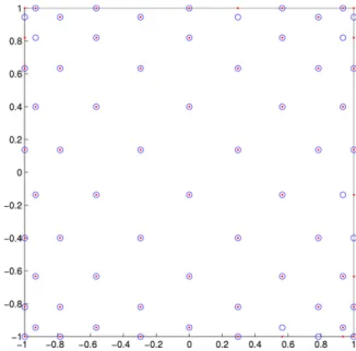
spacing) in the

(9)

Fig. 1. N=66 approximate Fekete points (dots) and Padua points (bullets) from a 11×12 Chebyshev–Lobatto grid at degreen=10 (they differ only by 4 points close to the top vertices).

Dubiner metric. In such a way we deal withM

=

O

(

n2

₎

_{instead of}_O

₍

_n4

₎

_{points, and the computational cost is pulled down}

by a factorn2_to_O

₍

_n6

₎

_{flops and}_O

₍

_n4

₎

_{storage. The qualitative idea behind this approach is that}_{Algorithm 1}_{will then select}

half of these points as approximate Fekete points, possibly maintaining the correct spacing.

It is worth to stress that both the qualitative strategies sketched above to generate the starting discretization via the conjectured spacing in the Dubiner metric, have indeed also a foundation in the theory of ‘‘admissible meshes’’ for polynomial approximation developed very recently by Calvi and Levenberg in [35]. Both the strategies, in fact, produce (weakly) admissible meshes (at least qualitatively), as tensor products of one-dimensional (weakly) admissible meshes. In [35] it is proved that maximizing the Vandermonde volume on such kind of meshes, gives approximate Fekete points that are (asymptotically) nearly as good as continuum Fekete points. An important fact is that the theory of [35] is applicable to many other multivariate compact domains, e.g. to domains that admit a Markov polynomial inequality, as well as to finite unions and products of such domains.

InTables 10–12we show at a sequence of low degrees the cubature and interpolation parameters of approximate Fekete points extracted byAlgorithm 2from a

(

2n2

+

1

)

×

(

2n2

+

1

)

uniform grid, and of those extracted from

(

n

+

1

)

×

(

n

+

2

)

Chebyshev–Lobatto and Gauss–Lobatto grids. Observe that following [35] the former is sufficiently dense to be an admissible mesh (see the proof of Thm.5 there), and the latter are tensor products of one-dimensional weakly admissible meshes. On the other hand, the latter are also (nearly for Gauss–Lobatto) equally spaced in the Dubiner metric(17). We use the product Chebyshev orthogonal basis (cf. [29]), suitably ordered, to construct the Vandermonde matrix. All the tests are done by an Intel-Centrino Duo processor 1.38 GHz with 1 Gb RAM, using Matlab 6.5 under Windows XP. To avoid possible confusion with the examples of the previous sections, we stress that here we extract approximate Fekete points with a fixed polynomial basis from different grids, whereas in the univariate examples we worked with different bases on a fixed grid.

In order to have a meaningful comparison, we report also the absolute value of the Vandermonde determinant (in the product Chebyshev basis) and the Lebesgue constant of the so-called ‘‘Padua points’’, and of a family of ‘‘Padua-like’’ points obtained from the Gauss–Lobatto tensorial grid (PdGL). We recall that the Padua points, recently studied in [33,36–39], are the first known optimal family for total degree bivariate polynomial interpolation, with a Lebesgue constant growing like O

(

log2n

)

. At a fixed degreen, they are the union of the two subgrids of a

(

n

+

1

)

×

(

n

+

2

)

Chebyshev–Lobatto grid, obtained by alternating odd and even indexes in one direction, seeFig. 1(indeed, there are four families of such points, one obtainable from the other by suitable rotations of the square). Their optimality is intimately related to the fact that they lie on a peculiar algebraic ‘‘generating’’ curve, see [36]. The ‘‘Padua-like’’ Gauss–Lobatto points, obtained in the same way as union of two subgrids of a

(

n

+

1

)

×

(

n

+

2

)

Gauss–Lobatto grid (seeFig. 2), are considered here for the first time.

We can see that the best approximate Fekete points seem those extracted from the Chebyshev–Lobatto tensorial grid inTable 12. The Lebesgue constants are estimated numerically on a 100

×

100 uniform control grid (a strange peak of the Lebesgue constant arises at degreen

=

16 after the iterative refinement, which however is present also inTable 11). The quadrature weights are not all positive, but their

`

1-norm remains close to 4 (the square area), that is the negative weights are few and small. InTables 10and11we see that also extraction from the other grids gives good results, but with the (much more dense) uniform grid we begin to have memory allocation problems already at relatively low degree (n

=

16 for iter

>

0 andn

=

20 already for iter

=

0: see the machine features quoted above).

(10)

Fig. 2. N=66 approximate Fekete points (dots) and Padua-like points (bullets) from a 11×12 Gauss–Lobatto grid at degreen=10 (they differ only by 9 points close to the boundary).

Table 10

Quality parameters ofN=((n+1)×(n+2))/2 approximate Fekete points extracted from a(2n2₊₁₎_×₍₂_n2₊₁₎_{uniform grid in}_Ω_{= [−}₁_,₁_]2_with

iterative refinement (product Chebyshev basis);∗ =‘‘out of memory’’.

n=4 n=8 n=12 n=16 n=20

iter (N=15) (N=45) (N=91) (N=153) (N=231)

cond(Vt₎ ₀ _2.1E₊₀₀ _2.1E₊₀₀ _2.1E₊₀₀ _2.1E₊₀₀ _∗

1 1.0E+00 1.0E+00 1.0E+00 ∗ ∗

2 1.0E+00 1.0E+00 1.0E+00 ∗ ∗

|det(V∗)| 0 3.0E+06 1.3E+27 4.9E+65 2.2E+125 ∗

1 3.0E+06 7.8E+26 3.6E+66 ∗ ∗

2 3.0E+06 7.8E+26 3.6E+66 ∗ ∗

Padua pts|det| 2.0E+06 1.6E+27 6.7E+66 5.0E+127 4.2E+211

kres(w)k2 0 2.2E−15 3.9E−15 5.9E−15 6.0E−15 ∗

1 1.7E−16 5.7E−17 2.6E−17 ∗ ∗

2 9.5E−17 5.0E−17 2.4E−17 ∗ ∗

P |wik| 0 5.05 4.32 5.31 4.11 ∗ 1 6.34 5.45 4.24 ∗ ∗ 2 6.34 4.95 4.20 ∗ ∗ Λn 0 5.27 10.6 22.6 28.1 ∗ 1 5.59 11.4 12.1 ∗ ∗ 2 5.59 11.4 12.1 ∗ ∗ Padua ptsΛn 4.41 6.21 7.45 8.41 9.20

The use of Chebyshev–Lobatto tensorial grids allows us to work without problems at much higher degrees, as we can see inTables 13and14. We report the Lebesgue constants of the approximate Fekete points (after one refinement iteration) at degrees 10

,

20

, . . . ,

60, and the corresponding quadrature and interpolation errors on the bivariate Runge test function, compared to those of the Padua and PdGL points. Notice the very good behavior of the quadrature formulas, which turn out to be more accurate than tensor-product Gaussian formulas and even of the few known minimal formulas, a phenomenon already discussed in [40] (see the error curves in Section 3.3 there).

4.2. Conclusions and perspectives

We have implemented (in Matlab) a method for computing approximate Fekete points, which is essentially based on a greedy algorithm for discrete maximization of Vandermonde determinants and uses only optimized tools of numerical linear algebra (QR-type factorizations of Vandermonde matrices on suitable discretization grids). The choice of the polynomial basis seems to play an important computational role, but it can be corrected and stabilized by discrete orthogonalization. SeeAlgorithms 1and2in Sections1and3.

(11)

Table 11

Quality parameters ofN=((n+1)×(n+2))/2 approximate Fekete points extracted from a(n+1)×(n+2)Gauss–Lobatto grid inΩ= [−1,1]2_with

iterative refinement (product Chebyshev basis); PdGL=Padua-like Gauss–Lobatto points.

n=4 n=8 n=12 n=16 n=20

iter (N=15) (N=45) (N=91) (N=153) (N=231)

cond(Vt₎ ₀ _2.6E₊₀₀ _2.6E₊₀₀ _2.5E₊₀₀ _2.4E₊₀₀ _2.3E₊₀₀

1 1.0E+00 1.0E+00 1.0E+00 1.0E+00 1.00E+00

2 1.0E+00 1.0E+00 1.0E+00 1.0E+00 1.00E+00

|det(V∗)| 0 2.0E+06 5.0E+26 5.4E+65 7.7E+124 1.0E+207

1 1.8E+06 1.3E+27 1.7E+65 6.6E+123 1.9E+209

2 1.8E+06 1.3E+27 1.7E+65 6.6E+123 1.9E+209

PdGL pts|det| 1.9E+06 1.3E+27 4.2E+66 2.2E+127 1.2E+211

kres(w)k2 0 2.2E−15 4.0E−15 5.4E−15 5.1E−15 7.3E−15

1 6.7E−16 5.8E−16 6.2E−16 4.2E−16 4.1E−16

2 6.7E−16 5.8E−16 6.2E−16 4.2E−16 4.1E−16

P |wik| 0 5.11 4.56 4.43 4.56 4.40 1 6.40 4.19 4.63 4.75 4.11 2 6.40 4.19 4.63 4.75 4.11 Λn 0 6.53 12.5 15.5 26.0 34.9 1 5.83 7.99 17.0 39.3 22.7 2 5.83 7.99 17.0 39.3 22.7 PdGL ptsΛn 5.20 8.53 11.3 13.7 15.8 Padua ptsΛn 4.41 6.21 7.45 8.41 9.20 Table 12

Quality parameters ofN=((n+1)×(n+2))/2 approximate Fekete points extracted from a(n+1)×(n+2)Chebyshev–Lobatto grid inΩ= [−1,1]2

with iterative refinement (product Chebyshev basis).

n=4 n=8 n=12 n=16 n=20

iter (N=15) (N=45) (N=91) (N=153) (N=231)

cond(Vt₎ ₀ _2.6E₊₀₀ _2.6E₊₀₀ _2.5E₊₀₀ _2.4E₊₀₀ _2.3E₊₀₀

1 1.0E+00 1.0E+00 1.0E+00 1.0E+00 1.0E+00

2 1.0E+00 1.0E+00 1.0E+00 1.0E+00 1.0E+00

|det(V∗)| 0 1.4E+06 6.4E+25 3.1E+65 3.1E+124 6.2E+206

1 1.4E+06 9.9E+26 4.5E+66 1.7E+125 2.9E+211

2 1.4E+06 9.9E+26 4.5E+66 1.7E+125 2.9E+211

kres(w)k2 0 2.3E−15 5.4E−15 6.1E−15 6.0E−15 7.5E−15

1 8.3E−16 5.9E−16 5.3E−16 5.0E−16 4.3E−16

2 8.3E−16 5.9E−16 5.3E−16 5.0E−16 4.3E−16

P |wik| 0 5.25 4.85 5.14 4.93 4.54 1 8.45 4.19 4.04 4.56 4.01 2 8.45 4.19 4.04 4.56 4.01 Λn 0 6.74 19.0 20.6 30.9 32.2 1 7.09 8.48 9.54 20.2 11.2 2 7.09 8.48 9.54 20.2 11.2 Padua ptsΛn 4.41 6.21 7.45 8.41 9.20 Table 13

Comparison of the Lebesgue constants inΩ = [−1,1]2_{: approximate Fekete points (obtained as in}_{Table 12}_{by 1 refinement iteration), Padua points,}

Padua-like Gauss–Lobatto points (PdGL).

n=10 n=20 n=30 n=40 n=50 n=60

Points (N=66) (N=231) (N=496) (N=861) (N=1326) (N=1891)

Approx Fek 9.01 11.2 12.9 37.9 38.2 40.6

Padua 6.88 9.20 10.7 11.9 12.9 13.7

PdGL 10.0 15.8 20.5 24.6 28.2 31.5

The numerical tests for the interval (Sections2and3) and for the square (Section4.1) have shown that such approximate Fekete points have very good features for algebraic quadrature and interpolation. Their Lebesgue constants grow slowly, and the associated quadrature weights, even though not all positive, show an

`

1-norm which remains close to the domain measure. The interval and the square are the only domains where optimal interpolation points are theoretically known, and indeed we have used such points for the purpose of comparison (in particular, the recently discovered ‘‘Padua points’’ for the square, see [33,36,37]).

(12)

Table 14

Absolute quadrature and interpolation errors for the bivariate version of the Runge function: approximate Fekete points (obtained as inTable 12by 1 refinement iteration), Padua points, Padua-like Gauss–Lobatto points (PdGL); the integral up to machine precision is 0.597388947274307.

n=10 n=20 n=30 n=40 n=50 n=60

Points (N=66) (N=231) (N=496) (N=861) (N=1326) (N=1891) Approx Fek

Quadr 2.0E−03 6.0E−05 2.3E−06 4.0E−07 1.3E−08 2.1E−09

Interp 3.9E+00 6.2E−01 9.9E−02 1.6E−02 1.4E−03 2.4E−04

Padua

Quadr 5.2E−04 1.3E−05 2.1E−07 1.3E−08 8.0E−10 5.9E−11

Interp 3.9E+00 6.2E−01 9.9E−02 1.6E−02 1.4E−03 2.4E−04

PdGL

Quadr 4.1E−04 1.3E−05 3.6E−07 2.4E−08 1.8E−09 1.6E−10

Interp 3.8E+00 5.9E−01 9.5E−02 1.6E−02 1.5E−03 2.5E−04

In the examples we have used a connection with the theory of metrics associated to polynomial inequalities and with the very recent theory of admissible meshes for polynomial approximation, see [18,31,35]. This connection, together with the relatively low computational complexity of the discrete method with respect to very costly maximizations in the continuum (cf. e.g. [19]), seems to open the way towards computation of good points for global high-degree interpolation and quadrature in many other standard and nonstandard multivariate domains. On the other hand, also local polynomial methods based on piecewise interpolation over standard and nonstandard partitions of the domains could benefit from this new approach.

References

[1] A. Sommariva, M. Vianello, Product Gauss cubature over polygons based on Green’s integration formula, BIT 47 (2007) 441–453.

[2] A. Sommariva, M. Vianello, Gauss–Green cubature and moment computation over arbitrary geometries, preprint, 2008 (available online at: http://www.math.unipd.it/~marcov/publications.html).

[3] A. Björk, Numerical Methods for Least Squares Problems, SIAM, 1996.

[4] G.H. Golub, C.F. Van loan, Matrix Computations, third ed., Johns Hopkins University Press, 1996.

[5] The Mathworks, MATLAB documentation set 2007 version (available online at:http://www.mathworks.com). [6] W. Gautschi, Moments in quadrature problems, Comput. Math. Appl. 33 (1997) 105–118.

[7] P.A. Businger, G.H. Golub, Linear least-squares solutions by householder transformations, Numer. Math. 7 (1965) 269–276. [8] LAPACK Users’ Guide, SIAM, 1999, (available online athttp://www.netlib.org/lapack).

[9] L. Bos, N. Levenberg, On the calculation of approximate Fekete points: the univariate case, Electron. Trans. Numer. Anal. 30 (2008) 377–397. [10] V.I. Krylov, Approximate Calculation of Integrals, Macmillan, 1962.

[11] T.J. Rivlin, An Introduction to the Approximation of Functions, Dover, 1969. [12] J.C. Mason, D.C. Handscomb, Chebyshev Polynomials, Chapman & Hall, 2003.

[13] A. Civril, M. Magdon-Ismail, Finding maximum volume sub-matrices of a matrix, Technical Report 07–08, Dept. of Comp. Sci., RPI, 2007 (available online at:www.cs.rpi.edu/research/pdf/07-08.pdf).

[14] G. Quintana-Ortí, X. Sun, C.H. Bischof, A BLAS-3 version of the QR factorization with column pivoting, SIAM J. Sci. Comput. 19 (1998) 1486–1494. [15] M. Dubiner, The theory of multidimensional polynomial approximation, J. Anal. Math. 67 (1995) 39–116.

[16] M. Reimer, Multivariate Polynomial Approximation, Birkhäuser, 2003.

[17] B. Sündermann, Lebesgue constants in Lagrangian interpolation at the Fekete points, Mitt. Math. Ges. Hamburg 11 (1983) 204–211. [18] L. Bos, N. Levenberg, S. Waldron, On the spacing of Fekete points for a sphere, ball or simplex, Indag. Math. 19 (2008) 163–176.

[19] M.A. Taylor, B.A. Wingate, R.E. Vincent, An algorithm for computing Fekete points in the triangle, SIAM J. Numer. Anal. 38 (2000) 1707–1720. [20] R. Pasquetti, F. Rapetti, Spectral element methods on unstructured meshes: Comparisons and recent advances, J. Sci. Comput. 27 (2006) 377–387. [21] J. Burkardt, Fekete: High order interpolation and quadrature in triangles, Matlab/Fortran90/C++ libraries (available online at:

http://people.scs.fsu.edu/~burkardt/m_src/fekete/fekete.html).

[22] I.H. Sloan, R.S. Womersley, Extremal systems of points and numerical integration on the sphere, Adv. Comput. Math. 21 (2004) 107–125. [23] R. Cools, An encyclopedia of cubature formulas, J. Complexity 19 (2003) 445–453.

[24] M.A. Taylor, B.A. Wingate, L. Bos, A cardinal function algorithm for computing multivariate quadrature points, SIAM J. Numer. Anal. 45 (2007) 193–205. [25] T. Kövari, C. Pommerenke, On the distribution of Fekete points, Mathematika 15 (1968) 70–75.

[26] D. Fasino, G. Inglese, On the spectral condition of rectangular Vandermonde matrices, Calcolo 29 (1992) 291–300.

[27] W. Gautschi, How (un)stable are Vandermonde systems?, in: R. Wong (Ed.), Asymptotic and Computational Analysis, in: Lecture Notes in Pure and Applied Mathematics, vol. 124, Marcel Dekker, 1990, pp. 193–210.

[28] L. Giraud, J. Langou, M. Rozloznik, J. van den Eshof, Rounding error analysis of the classical Gram–Schmidt orthogonalization process, Numer. Math. 101 (2005) 87–100.

[29] C.F. Dunkl, Y. Xu, Orthogonal Polynomials of Several Variables, in: Encyclopedia of Mathematics and its Applications, vol. 81, Cambridge University Press, 2001.

[30] L. Bos, N. Levenberg, S. Waldron, Metrics associated to multivariate polynomial inequalities, in: M. Neamtu, E.B. Saff (Eds.), Advances in Constructive Approximation, Nashboro Press, Nashville, 2004, pp. 133–147.

[31] L. Bos, N. Levenberg, S. Waldron, Pseudometrics, distances and multivariate polynomial inequalities, J. Approx. Theory 153 (2008) 80–96. [32] L. Bos, Multivariate interpolation and polynomial inequalities, Ph.D. course held at the University of Padua, 2001, unpublished.

[33] M. Caliari, S. De Marchi, M. Vianello, Bivariate polynomial interpolation on the square at new nodal sets, Appl. Math. Comput. 161 (2005) 261–274. [34] L. Bos, M.A. Taylor, B.A. Wingate, Tensor product Gauss–Lobatto points are Fekete points for the cube, Math. Comp. 70 (2001) 1543–1547. [35] J.P. Calvi, N. Levenberg, Uniform approximation by discrete least squares polynomials, J. Approx. Theory 152 (2008) 82–100.

[36] L. Bos, M. Caliari, S. De Marchi, M. Vianello, Y. Xu, Bivariate Lagrange interpolation at the Padua points: The generating curve approach, J. Approx. Theory 143 (2006) 15–25.

(13)

[37] L. Bos, S. De Marchi, M. Vianello, Y. Xu, Bivariate Lagrange interpolation at the Padua points: The ideal theory approach, Numer. Math. 108 (2007) 43–57.

[38] M. Caliari, S. De Marchi, M. Vianello, Bivariate Lagrange interpolation at the Padua points: Computational aspects, J. Comput. Appl. Math. 221 (2008) 284–292.

[39] M. Caliari, S. De Marchi, M. Vianello, Padua2D: Bivariate Lagrange interpolation at Padua points on bivariate domains, ACM Trans. Math. Software 35-3 (2008).