Robust Weighted LAD Regression
Avi Giloni, Jeffrey S. Simonoff, and Bhaskar Sengupta∗
February 25, 2005
Abstract
The least squares linear regression estimator is well-known to be highly sensitive to unusual observations in the data, and as a result many more robust estimators have been proposed as alternatives. One of the earliest proposals was least-sum of absolute deviations (LAD) regression, where the regression coefficients are estimated through minimization of the sum of the absolute values of the residuals. LAD regression has been largely ignored as a robust alternative to least squares, since it can be strongly affected by a single observation (that is, it has a breakdown point of 1/n, where n is the sample size). In this paper we show that judicious choice of weights can result in a weighted LAD estimator with much higher breakdown point. We discuss the properties of the weighted LAD estimator, and show via simulation that its performance is competitive with that of high breakdown regression estimators, particularly in the presence of outliers located at leverage points. We also apply the estimator to several real data sets.
Keywords: Breakdown point; Leverage points; Outliers; Robust regression.
∗
Avi Giloni is Assistant Professor, Sy Syms School of Business, Yeshiva University, 500 West 185th St, New York, NY 10033 (e-mail: [email protected]). Jeffrey S. Simonoff is Professor, Leonard N. Stern School of Business, New York University, 44 West 4th Street, New York, NY, 10012 (e-mail: [email protected]). Bhaskar Sengupta is Section Head, Complex Systems Mod-eling, ExxonMobil Research and Engineering, 1545 Route 22 East, Annandale, NJ 08801 (e-mail: [email protected]). This work was done while he was at Yeshiva University. The au-thors would like to thank Steve Portnoy for helpful discussion of this material.
1
Introduction
The linear regression problem is certainly one of the most important data analysis
situa-tions (if not the most important). In this situation the data analyst is presented with n
observations of a response variable y and some number pof predicting variables x1, . . . , xp
satisfying
y=Xβ+ε, (1)
whereε is a vector of errors and
y= y1 · · · yn , X= x11 · · · x1p · · · · · · xn 1 · · · xnp = x1 · · · xn = (x1, . . . ,xp), ε= ε1 · · · εn
(note that usuallyx1 is a column of ones, but this is not required). We assume that X is
of full rank (that is,r(X) =p).
It is well-known that if the errorsεare normally distributed with constant variance the
optimal estimator ofβ is the ordinary least squares (OLS) estimator, based on minimizing
the`2-norm ky−Xβbk2 =Pni=1(yi−xiβb)2 of the residuals. Unfortunately, it is also
well-known that the least squares estimator is very nonrobust, being highly sensitive to unusual
observations in the y space (outliers) andX space (leverage points).
A way of quantifying this sensitivity is through the notion of the breakdown point of
a regression estimator (Hampel, 1968). Suppose we estimate the regression parametersβ
by some technique τ from data (X,y), yielding the estimate βτ. If we contaminate m
(1 ≤m < n) rows of the data in a way so that row i is replaced by some arbitrary data
e xi,yei
, we obtain some new data
e X,ey
. The same technique τ applied to
e X,ey yields estimatesβτ e X,ey
that are different from the original ones. We can use any normk · kon
Rp to measure the distance
βτ e X,ey −βτ
of the respective estimates. If we vary over
all possible choices of contamination then this distance either stays bounded or not. Let
b(m, τ,X,y) = sup e X,ye βτ e X,ey −βτ
be the maximum bias that results when we replace at mostm of the original data xi, y i
by arbitrary new ones. The breakdown point of τ is then defined as
α(τ,X,y) = min 1≤m<n nm n :b(m, τ,X,y) is infinite o , (2)
the minimum proportion of rows of (X,y) that if replaced by arbitrary new data make the
regression technique τ break down. The minimum possible value of the breakdown point
is 1/n and the maximum value is .5 (the latter value since otherwise it is impossible to
distinguish between the uncontaminated data and the contaminated data). Clearly, the larger the breakdown point, the more robust is the regression estimator.
The least squares regression estimator has breakdown 1/n, and many alternative estima-tors have been proposed to provide more robust regression estimation. One of the earliest
proposals was regression performed through minimization of the `1 norm of the residuals,
ky−Xβbk1=Pin=1|yi−xiβb|, also called least-sum of absolute deviations (LAD) regression.
There is a good deal of empirical evidence going back more than 30 years that LAD regres-sion is more robust than OLS in the presence of fat-tailed errors (see, e.g., Sharpe, 1971). Despite this, LAD regression has gained relatively little favor in the robustness statistical literature, for several perceived reasons:
1. LAD estimation is more than difficult than OLS estimation, because of the nondiffer-entiability of the criterion function. In fact, as Portnoy and Koenker (1997) pointed out, modern linear programming techniques have made the computation time of LAD regression competitive with, or even superior to, OLS even for extremely large data sets. This can be contrasted with high breakdown regression estimators, which are far more computationally intensive than OLS (Rousseeuw and Leroy, 1987; Hawkins and Olive, 2002). As an example of the gains these new methods can provide, LAD estimation for a dataset with 100,000 observations and 100 variables takes more than 12 minutes using the Barrodale-Roberts modified simplex algorithm and only 30 sec-onds using the Frisch-Newton interior point algorithm on a Pentium 4 PC (3.2GHz
2. The asymptotic theory for LAD regression is not as well-developed as for OLS re-gression. While this is true to a certain degree, it is also true for high-breakdown regression estimators.
3. The LAD regression estimator is not at all robust to observations with unusual pre-dictor values; that is, it has a low breakdown point.
It is this final claim that is the starting point for this paper. In the next section, we discuss what is known about the breakdown of LAD regression, focusing on recent exact results. We discuss how the use of a weighted version of LAD regression can improve its robustness considerably, and describe an algorithm for choosing weights that leads to such improvements. In Section 3 we give the asymptotic properties of the resultant estimators, and examine finite-sample properties using Monte Carlo simulations. We apply the method to several data sets in Section 4. We conclude the paper with discussion of potential future work.
2
LAD Regression and Breakdown
If contamination is permitted in both the predictor and response variables, the breakdown
point of LAD is the same as that of OLS, 1/n(see, e.g., Rousseeuw and Leroy, 1987, page 12).
LAD regression is, however, more robust than least squares in the following sense. Define the finite sample breakdown point of the LAD estimator to be the breakdown point of LAD
regression with a fixed design matrixXand contamination restricted only to the dependent
variable y, denoted by α(τ,y|X). This is the ordinary breakdown (2) for given predictor
matrix X. This is a natural criterion in the regression context, since standard regression
theory proceeds based on conditioning on the observed values of the predictors. The finite sample breakdown point, or conditional breakdown point, was introduced in Donoho and
Huber (1983). Mizera and M¨uller (2001) and Giloni and Padberg (2004) showed that the
finite sample breakdown point of LAD regression can be greater than 1/n, depending on
the predictor values, with the former authors discussing how X can be chosen to increase
be calculated using a mixed integer program, and described an algorithm for solving it; Giloni, Sengupta, and Simonoff (2004) proposed an alternative algorithm similar to that of
Mizera and M¨uller (2001) that is very efficient for large samples when pis small.
Ellis and Morgenthaler (1992) appear to be the first to mention that the introduction of weights can improve the finite sample breakdown point of LAD regression (by downweight-ing observations that are far from the bulk of the data), but they only show this for very small data sets. Giloni, Sengupta, and Simonoff (2004) examined this question in more detail. The weighted LAD (WLAD) regression estimator is defined to be the minimizer of
n
X
i=1
wi|yi−xiβ|, (3)
This estimation problem can be formulated as a linear program, min n X i=1 wi r+i +ri− (4) such that Xβ+r+−r−=y β free,r+≥0,r−≥0.
Here, the residual ri associated with observationiis multiplied by some weight,wi, where
we assume that 0 < wi ≤ 1 without loss of generality. In the formulation of the linear
program the residualsrare replaced by a differencer+−r−of nonnegative variables. Since
r+i −r−i = yi−xiβ
, and by the simplex method either ri+>0 orr−i >0 but not both,
then|wi r+i −ri−
|=wi r+i +r−i
. Therefore, transforming the data by setting ˜xi,˜yi
= wi xi, yi , implies ˜yi−x˜iβ =wi ri+−r−i
. This means that the linear program (4) can be reformulated as
min eTnr++eTnr−
such that wixiβ+r+−r− =wiyi fori= 1, . . . , n
β free,r+≥0,r−≥0.
That is, weighted LAD regression can be treated as LAD regression with suitably trans-formed data, and determining the breakdown of weighted LAD regression with known
The problem of choosing weightswto maximize the breakdown of the resultant weighted LAD estimator is a nonlinear mixed integer program. Giloni, Sengupta, and Simonoff (2004) showed that this problem is equivalent to a problem related to the knapsack problem, and solved a specific form of the problem for the simple regression case with a uniform design, resulting in a WLAD breakdown over 30% (LAD regression has a 25% breakdown point in this situation). They also proposed a simple weighting scheme for multiple regression that yields breakdown points over 20% for various two-predictor problems. We propose here an improved weighting scheme that is fast computationally and leads to higher breakdown values. As was noted by Ellis and Morgenthaler (1992), the goal is to downweight observa-tions that are outlying in the predictor space (that is, are leverage points). Unfortunately, usual measures of leverage suffer from masking, in that multiple leverage points near each other can cause them to “hide” each other. High-breakdown measures of leverage can be calculated, but these are computationally intensive.
We will instead use conventional measures of leverage, but will measure outlyingness relative to what is (hopefully) a clean subset of the data. We define this subset to be the set
of`observations that are closest to the coordinatewise medians, where distance is the sum of
coordinatewise distances, and the variables have all been scaled to be in the range [0,1]. The
size`should be large enough to include much of the data, but small enough so that it doesn’t
include outlying observations; we use ` = .6n here. The notion of identifying outlying
observations by defining a clean subset of the data and then measuring the distance of observations relative to that subset was introduced by Rosner (1975) for univariate Gaussian data. The first application of this idea to multivariate and regression data appears to have been in Simonoff (1991). Other applications of this idea for multivariate and regression data can be found in Hadi (1992, 1994), Hadi and Simonoff (1993), Billor, Hadi, and Velleman (2000), and Atkinson and Riani (2000).
The definition of the clean subset used here is that used by Billor, Hadi, and Velleman (2000) as version 2 of their algorithm for finding a clean subset of a multivariate data set
(page 285), and as they note this is a robust method of choosing the clean subset. Let XS
subset ishi=xi(XS0XS)−1xi0, using the usual (least squares) notion of leverage. Since the
leverage is proportional to the squared Mahalanobis distance (Chatterjee and Hadi, 1988,
page 102), the weight is taken to bewi =
p
minj(hj)/hi; that is, it is inversely proportional
to the distance from the clean subset.
WLAD regression is a particular example of generalized M (GM)-estimation (Mallows, 1975). It is known that the maximum breakdown point of all GM-estimators decreases as
a function of p (Maronna, Bustos, and Yohai, 1979), implying that the breakdown point
of WLAD regression cannot be arbitrarily high for models with many predictors. In the next section we use Monte Carlo simulations to study the properties of WLAD regression, and show that despite this, WLAD estimation can be competitive with high breakdown
estimation even for reasonably large values ofp.
3
The Properties of WLAD Regression Estimation
We begin this section with discussion of the asymptotic properties of the WLAD estimator. Consider again the regression model (1), and assume that the errors are independent and
identically distributed with cumulative distribution functionF. Assume that maxkxik=
o(n1/4), F is twice differentiable at 0, and f(0) = F0(0) > 0. Let βˆw be the WLAD
estimator ofβ. LetW= diag(w1, . . . , wn), and assume that the weights are known positive
values that satisfy maxwi =O(1) and maxwi−1 =O(1).
Theorem 1 Asn→ ∞,√n( ˆβw−β) is asymptoticallyp-variate normal with mean 0 and covariance matrix
Q−1(X0W2X)Q−1ω2,
where Q= limn→∞X0WX/nand ω = [2f(0)]−1.
The proof of this theorem is given in the Appendix. The implication of this theorem is that
confidence regions for β can be constructed based on ˆβw using the estimated asymptotic
covariance, (X0WX)−1(X0W2X)(X0WX)−1ωˆ2, where ω is estimated in some reasonable
way. In the simulations that follow we use a kernel estimator to estimate f(0), and hence
We explore the finite-sample properties of WLAD regression using Monte Carlo simu-lations, performed using the R package (R Development Core Team, 2004). In addition to the WLAD estimator, we also report results for least squares, (unweighted) LAD, and MM estimators. The MM estimator (Yohai, 1987) uses an inefficient high-breakdown method as an initial estimate, but then uses M-estimation to improve efficiency while still maintain-ing a high breakdown point. We also included an M-estimator (Huber, 1973) and the least trimmed squares (LTS) high breakdown estimator (Rousseeuw, 1985) in the simulations, but the MM estimator consistently outperformed both, so we do not report those results here.
The (W)LAD estimators were constructed using the quantreg package (Koenker, 2004),
while the LTS and MM estimators were constructed using theMASSpackage (Venables and
Ripley, 2002). We examine various values of sample sizenand number of predictorsk(note
thatp=k+ 1, as the models include an intercept term), and different outlier/leverage point
proportion and position combinations. Predictors were generated multivariate normal (with each variable having mean 7.5 and standard deviation 4), with certain observations being modified to be leverage points in some situations, and 500 simulations replications were generated for each setting. All regression functions had intercept equal to 0 and all slopes equal to 5, with variance of the Gaussian errors equal to 1.
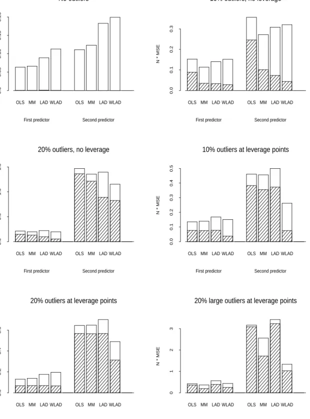
Figure 1 summarizes the results of simulations where n = 40 and k = 2. Each bar’s
height represents n×M SE, where M SE is the mean squared error of the slope estimate,
separated by predictor, with the shaded portion corresponding to squared bias and the unshaded portion corresponding to variance. Although both predictors were generated to have variance equal to 16, by random chance the second predictor had much lower variability
(sample variance 10.1), resulting in higher values of n×M SE for that predictor’s slope
estimate for all methods. As can be seen in the figure, the difference in variability of the predictors affects the relative performance of the methods.
When there are no outliers, all of the estimators are (virtually) unbiased, and relative efficiency drives the results. As expected, OLS is most efficient, with the MM estimator close. The LAD estimators are less efficient, with WLAD having highest variability (as would be expected, since observations with predictor values farthest from the center are
downweighted, and it is these observations that increase efficiency). Relative performance changes markedly in the presence of outliers however, with the nonrobust OLS estimator no longer effective. The first five plots refer to outliers with mean 3 standard deviations from the true expected value, while the last (“large outliers”) refers to outliers with mean 7 standard deviations from the true value. The last three plots refer to situations where the observations with outliers first had their predictor values adjusted to make them leverage points (the predictor values were centered roughly 4 standard deviations from the predictor mean). Given that the weighting scheme of the WLAD estimator is designed to downweight leverage points, it is not surprising to see much better performance for WLAD in this situation compared to LAD (in fact, the breakdown point of LAD is 17.5% while that of WLAD is 22.5%, so deteriorating performance for LAD in the 20% outliers case would be expected). That breakdown is not the entire story, however, is clear from the much better performance of WLAD compared to MM, especially when the outliers are at leverage points. This is being driven by much lower squared bias, although the variance of WLAD is also lower when there are 20% large outliers at the leverage points.
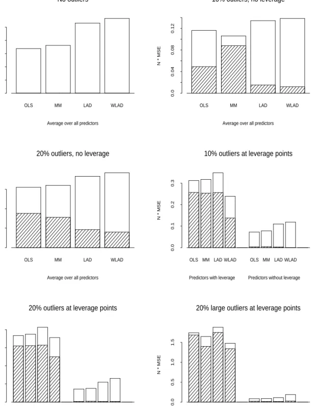
Figure 2 gives corresponding results where n = 100 and k = 6. Although it is not
feasible to calculate exact breakdown values for the (W)LAD estimators, upper bounds on those values can be determined (by running the mixed integer program for many iterations, but not to convergence), and they are 16% (for LAD) and 20% (for WLAD), respectively, in this case for the designs with 20% leverage points. Despite the fact that the breakdown point for WLAD is not greater than the observed percentage of generated outlier obser-vations (implying that breakdown can occur), it is still an effective estimator, once again outperforming the MM estimator in the presence of leverage points. Once again, the es-timator exhibits good bias properties, although that is outweighed by high variance when
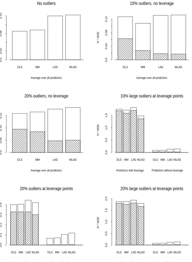
the data do not contain leverage points. Figure 3 gives results for n = 1000 and k= 20.
Even in this case, where the large number of predictors implies a maximum breakdown point of WLAD less than 2% for the design with 20% leverage points, the performance of WLAD is similar to that seen earlier, with the estimator outperforming the MM estimator for large outliers in the presence of leverage points. Thus, it is apparent that the goal of
increasing the breakdown point of the estimator is a reasonable one, even when there are more outliers than the breakdown value. This will also be evident in several of the data examples discusses in the next section.
We also examined the usefulness of the asymptotic distribution derived in Theorem 1 as a tool for inference, by examining the properties of hypothesis tests based on the approximate
normal distribution. Construction of such tests requires estimatingω = [2f(0)]−1, which is
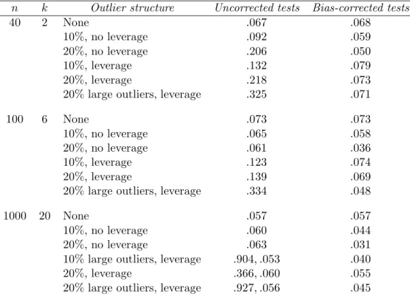
done here using a kernel density estimate (see, e.g., section 3.1 of Simonoff, 1996), with the amount of smoothing chosen using the bandwidth selector of Sheather and Jones (1991). The adequacy of the approximation was evaluated by determining the average rejection proportions (empirical sizes) of Wald (Gaussian-based) tests for each coefficient of the actual null value at a nominal .05 level and then averaging over all slopes, so the goal would be tests with size close to .05.
Results for the simulation situations previously examined are summarized in Table 1. We give results for the actual tests, and also for tests where the coefficient estimates are recentered at the null value, so that the bias of the estimators does not affect performance.
For the n = 1000 case with leverage points, separate average empirical sizes are given
for the predictors with and without leverage points for the uncorrected tests, since their performances are very different. It can be seen that while the bias seen earlier (especially in the leverage point case) results in very anticonservative tests (which would presumably also be true for the other estimators, since they are even more biased), when this bias is corrected, the tests have size reasonably close to .05. Thus, the evidence suggests that the assumption of a Gaussian distribution for the coefficient estimator, and the implied estimates of standard errors of the coefficient estimates, are reasonable even for small samples.
4
Application to Real Datasets
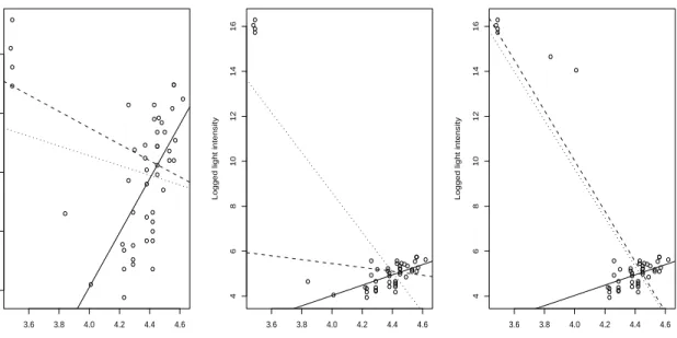
In this section we apply the WLAD estimator to several well-known datasets from the ro-bustness and outlier identification literature. The Hertzsprung-Russell stars data (Rousseeuw and Leroy, 1987, page 27) consist of measurements of the logarithm of light intensity versus logarithm of effective surface temperature for 47 stars. The data are given in the leftmost
plot in Figure 4. Although there is a direct relationship between the two variables for most of the observations, four stars have low temperature with high light intensity (these are so-called “red giant” stars). The OLS fit (dotted line) is drawn to these outliers, as is the LAD fit (dashed line), but the WLAD fit (solid line) follows the general pattern of the points well (note that the LAD estimate actually passes through one of the outliers). It might be thought that the improved performance of WLAD over LAD is because of its higher breakdown point, but this is not, in fact, the case. The breakdown point of LAD here is 10.6% (5/47), so the four observed outliers are not enough to break down the estimator. This can be seen in the middle plot of Figure 4, where the four outliers have had their responses adjusted upwards by 10. The OLS line continues to follow the points, but the LAD line is virtually unchanged (and no longer passes through any of the outliers), because it has not broken down (not surprisingly, the WLAD line is unchanged). Thus, WLAD provides a better fit than LAD even when LAD has not broken down. On the other hand, the improved breakdown point of WLAD (which is 14/47 = 29.8%) becomes apparent if two more values are perturbed upwards (the rightmost plot of Figure 4). With six outliers LAD has broken down, and tracks the unusual points in a similar way to OLS (once again passing through one of them), while WLAD still follows the bulk of the points.
Hawkins, Bradu, and Kass (1984) constructed an artificial three-predictor data set with 75 observations, where outliers were placed at cases 1–10. The LAD estimator has break-down point 10.7% (8/75) and breaks break-down, with the fitted regression hyperplane going through one of the outlier points (it goes through cases 5, 20, and 32). In contrast the WLAD estimator, with breakdown point 20% (15/75) works well, going through cases 18, 25, and 30, with each of the outlier observations having absolute residual at least 2.3 times that of any of the clean points. The fitted WLAD regression is
Y =−0.446 + 0.159X1+ 0.090X2−0.032X3,
withz-statistics for the three slopes being 1.15, 0.78, and−0.37, respectively. That is, there
is little evidence for any relationship here, which is consistent with the way the data were
11-75 are statistically significant (in contrast to the fit on all of the observations, where the
outliers result in variablesX2 and X3 being significant predictors).
The final data set examined here is the modified wood gravity of Rousseeuw (1984).
These data are based on a real data set (with n = 20 and k = 5), but were modified to
have outliers at cases 4, 6, 8, and 19. Both LAD and WLAD have the same breakdown point (15% = 3/20), but despite this, while LAD performs poorly (passing through the outlier case 8), WLAD performs well, with each of the four outlier cases having absolute residual more than 7.7 times that of any of the clean points. Thus, the WLAD weighting is beneficial even when breakdown is not improved. The fitted WLAD regression is
Y = 0.387 + 0.321X1−0.422X2−0.541X3−0.336X4+ 0.523X5,
withz-statistics for the five slopes being 8.50,−2.64,−15.18,−6.32, and 7.79, respectively.
An OLS fit on the clean data also identifies predictors 1, 3, 4, and 5 as being most important, although in that case the coefficient for variable 2 is not statistically significant (in contrast to an OLS fit on the entire data set, where variables 4 and 5 are insignificant, because of the effect of the outliers).
5
Conclusion
In this paper we have proposed a weighted version of LAD regression designed to increase the breakdown of the estimator that is easy to compute and has performance competi-tive with high breakdown estimators, particularly in the presence of leverage points. These weighting ideas also apply to other estimators. Given the good bias properties of the WLAD estimator, it is reasonable to wonder if a similar weighting scheme used for a more efficient GM-estimator, such as that of Krasker and Welsch (1982), would reduce the variance while preserving robustness, and be even more effective than WLAD. The LAD estimator is a special case of regression quantile estimators (Koenker and Bassett, 1978; Koenker, 2000), which have been shown to be useful in highlighting interesting structure in regression prob-lems, including nonnormality and heteroscedasticity in the error distribution; it would be interesting to see if weighted versions of such estimators would be more resistant to the
effects of unusual observations.
Appendix
Consider the model
y=Xβ+∆nu,
where ∆n = diag(δ1, . . . , δn), β ∈ <p, and u is a vector of independent and identically
distributed errors with cumulative distribution functionF. Assume that theδis are known
values satisfying maxδi = O(1) and maxδi−1 = O(1), and that maxkxik = o(n1/4).
Assume thatF is twice differentiable at 0, and f(0) =F0(0)>0. LetQn=X0∆−1n X/n=
Q+O(n−1/4logn). Let ˆβ be the least absolute deviation (LAD) estimator of β that
minimizes n X i=1 |yi−xiβ|. Lemma 1 As n→ ∞, ˆ β−β= n −1Q−1 n f(0) n X i=1 xi0Ψ(ui) +O((logn/n)3/4), where Ψ(x) =I(x <0)−.5.
Proof: This result follows from an adaptation of the proof of Theorem 2.1 of Zhou and
Portnoy (1998) (hereafter ZP). In that theorem the multipliersδi are estimated based on
a linear function of a parameter vector γ, so the results quoted here are based on taking
ˆ
γ=γ in that proof. Let Wn(t) =Pni=1xi0Ψ(ui). By Lemma A.1 of ZP,
Wn( ˆβ−β) =O(n−3/4). (5)
LetMn=c0n−1/2(logn)1/2. Then, by Lemma A.2 of ZP,
sup
ktk≤Mn
kWn(t)−Wn(0) +f(0)Qtk=Op(n−3/4(logn)3/4). (6)
Substituting ˆβ−β fort in (6) and then substituting (5) into (6) gives
The result of the lemma then follows.
The next lemma uses this result to establish the asymptotic distribution of the LAD estimator under known heteroscedasticity.
Lemma 2 As n → ∞, √n( ˆβ−β) is asymptotically p-variate normal with mean 0 and covariance matrix
Q−1(X0X)Q−1ω2,
where Q is defined as in Lemma 1 and ω= [2f(0)]−1.
Proof: This is a direct consequence of Lemma 1. The Central Limit Theorem implies asymptotic normality, and since
V n X i=1 xi0Ψ(ui) ! = (X0X)/4
the result follows.
These results then allow us to derive the asymptotic distribution of the WLAD estimator under the usual i.i.d. conditions, as follows.
Proof of Theorem 1: This follows from Lemma 2. Let ˜X=WX and ˜y =Wy. Then the weighted LAD estimation problem is equivalent to unweighted estimation for the model
˜
y= ˜Xβ+Wε.
Lemma 2 implies that √n( ˆβw −β) is asymptotically p-variate normal with mean 0 and
covariance matrix
Q−1( ˜X0W2X˜)Q−1ω2,
whereQ= limn→∞X˜0W−1X˜/n. Substituting WXfor ˜Xgives the result.
References
Atkinson, A. and Riani, M. (2000),Robust Diagnostic Regression Analysis, Springer-Verlag,
Billor, N., Hadi, A.S., and Velleman, P.F. (2000), “BACON: blocked adaptive
computa-tionally efficient outlier nominators,” Computational Statistics and Data Analysis, 34,
279–298.
Chatterjee, S. and Hadi, A.S. (1988),Sensitivity Analysis in Linear Regression, Wiley, New
York.
Donoho, D.L. and Huber, P.J. (1983), “The notion of breakdown point,” in P. Bickel, K.
Doksum and J.L. Hodges, eds., A Festschrift for Erich Lehmann, Wadsworth, Belmont,
CA, 157–184.
Ellis, S.P. and Morgenthaler, S. (1992), “Leverage and breakdown in L1-regression,”Journal
of the American Statistical Association,87, 143–148.
Giloni, A. and Padberg, M. (2004), “The finite sample breakdown point of `1-regression,”
SIAM Journal on Optimization,14, 1028–1042.
Giloni, A., Sengupta, B., and Simonoff, J.S. (2004), “A mathematical programming ap-proach for improving the robustness of LAD regression,” unpublished manuscript.
Hadi, A.S. (1992), “Identifying multiple outliers in multivariate data,”Journal of the Royal
Statistical Society, Ser. B,54, 761–771.
Hadi, A.S. (1994), “A modification of a method for the detection of outliers in multivariate
samples,”Journal of the Royal Statistical Society, Ser. B,56, 393–396.
Hadi, A.S. and Simonoff, J.S. (1993), “Procedures for the identification of multiple outliers
in linear models,” Journal of the American Statistical Association,88, 1264–1272.
Hampel, F.R. (1968), Contributions to the Theory of Robust Estimation. PhD. Thesis,
University of California, Berkeley.
Hawkins, D.M., Bradu, D., and Kass, G.V. (1984), “Location of several outliers in multiple
Hawkins, D.M. and Olive, D.J. (2002), “Inconsistency of resampling algorithms for
high-breakdown regression estimators and a new algorithm,”Journal of the American
Statis-tical Association,97, 136–159.
Huber, P.J. (1973), “Robust regression: Asymptotics, conjectures, and Monte Carlo,”
An-nals of Statistics,1, 799–821.
Koenker, R. (2000), “Galton, Edgeworth, Frisch, and prospects for quantile regression in
econometrics,”Journal of Econometrics,95, 347–374.
Koenker, R. (2004), quantreg: Quantile Regression, R package version 3.70
(http://www.econ.uiuc.edu/ roger/research/rq/rq.html).
Koenker, R. and Bassett, G., Jr. (1978), “Regression quantiles,”Econometrica,46, 33–50.
Krasker, W.S. and Welsch, R.E. (1982), “Efficient bounded-influence regression estimation,”
Journal of the American Statistical Association,77, 595–604.
Mallows, C.L. (1975), “On some topics in robustness,” Technical Memorandum, Bell Tele-phone Laboratories, Murray Hill, NJ.
Maronna, R.A., Bustos, O.H., and Yohai, V.J. (1979), “Bias- and efficiency-robustness of general M-estimators for regression with random carriers,” in T. Gasser and M.
Rosen-blatt, eds., Smoothing Techniques for Curve Estimation, Lecture Notes in Mathematics
757, Springer-Verlag, Berlin, 91–116.
Mizera, I. and M¨uller, C.H. (2001), “The influence of the design on the breakdown points
of `1-type M-estimators,” in A. Atkinson, P. Hackl, and W. M¨uller, eds., MODA6 –
Advances in Model-Oriented Design and Analysis, Physica-Verlag, Heidelberg, 193–200. Portnoy, S. and Koenker, R. (1997), “The Gaussian hare and the Laplacian tortoise:
com-putability of squared-error versus absolute-error estimators,”Statistical Science,12, 279–
R Development Core Team (2004),R: A language and environment for statistical computing,
R Foundation for Statistical Computing, Vienna, Austria (http://www.R-project.org).
Rosner, B. (1975), “On the detection of many outliers,”Technometrics,17, 221–227.
Rousseeuw, P.J. (1984), “Least median of squares regression,” Journal of the American
Statistical Association,79, 871–880.
Rousseeuw, P.J. (1985), “Multivariate estimation with high breakdown point,” in
Mathe-matical Statistics and Applications(Vol. B), eds. W. Grossmann, G. Pflug, I. Vincze, and W. Wertz, Dordrecht, Reidel, 283–297.
Rousseeuw P.J. and Leroy A.M. (1987), Robust Regression and Outlier Detection, Wiley,
New York.
Sharpe, W.F. (1971), “Mean-absolute-deviation characteristic lines for securities and
port-folios,”Management Science,18, B1–B13.
Sheather, S.J. and Jones, M.C. (1991), “A reliable data-based bandwidth selection method
for kernel density estimation,”Journal of the Royal Statistical Society, Ser. B,53, 683–
690.
Simonoff, J.S. (1991), “General approaches to stepwise identification of unusual values in
data analysis,” in W. Stahel and S. Weisberg, eds., Directions in Robust Statistics and
Diagnostics: Part II, Springer-Verlag, New York, 223–242.
Simonoff, J.S. (1996),Smoothing Methods in Statistics, Springer-Verlag, New York.
Venables, W.N. and Ripley, B.D. (2002),Modern Applied Statistics with S, 4th ed., Springer,
New York.
Yohai, V.J. (1987), “High breakdown-point and high efficiency robust estimates for
regres-sion,” Annals of Statistics,15, 642–656.
Zhou, K.Q. and Portnoy, S.L. (1998), “Statistical inference on heteroscedastic models based
Table 1: Average empirical size of tests for slope coefficients (nominal sizeα=.05). n k Outlier structure Uncorrected tests Bias-corrected tests
40 2 None .067 .068
10%, no leverage .092 .059
20%, no leverage .206 .050
10%, leverage .132 .079
20%, leverage .218 .073
20% large outliers, leverage .325 .071
100 6 None .073 .073
10%, no leverage .065 .058
20%, no leverage .061 .036
10%, leverage .123 .074
20%, leverage .139 .069
20% large outliers, leverage .334 .048
1000 20 None .057 .057
10%, no leverage .060 .044
20%, no leverage .063 .031
10% large outliers, leverage .904, .053 .040
20%, leverage .366, .060 .055
Figure 1: Results of simulations withn= 40 observations and two predictors. Bars represent
n×mean squared error for each estimator, separated into squared bias (shaded) and variance
(unshaded) parts.
OLS MM LAD WLAD OLS MM LAD WLAD
0.0 0.05 0.10 0.15 0.20 No outliers N * MSE
First predictor Second predictor
OLS MM LAD WLAD OLS MM LAD WLAD
0.0 0.1 0.2 0.3 10% outliers, no leverage N * MSE
First predictor Second predictor
OLS MM LAD WLAD OLS MM LAD WLAD
0.0 0.5 1.0 1.5 20% outliers, no leverage N * MSE
First predictor Second predictor
OLS MM LAD WLAD OLS MM LAD WLAD
0.0 0.1 0.2 0.3 0.4 0.5
10% outliers at leverage points
N * MSE
First predictor Second predictor
OLS MM LAD WLAD OLS MM LAD WLAD
0.0
0.2
0.4
0.6
20% outliers at leverage points
N * MSE
OLS MM LAD WLAD OLS MM LAD WLAD
0
1
2
3
20% large outliers at leverage points
Figure 2: Results of simulations withn= 100 observations and six predictors. Bars
repre-sent n× mean squared error for each estimator, separated into squared bias (shaded) and
variance (unshaded) parts.
OLS MM LAD WLAD
0.0
0.04
0.08
No outliers
N * MSE
Average over all predictors
OLS MM LAD WLAD
0.0 0.04 0.08 0.12 10% outliers, no leverage N * MSE
Average over all predictors
OLS MM LAD WLAD
0.0 0.05 0.10 0.15 20% outliers, no leverage N * MSE
Average over all predictors
OLS MM LAD WLAD OLS MM LAD WLAD
0.0
0.1
0.2
0.3
10% outliers at leverage points
N * MSE
Predictors with leverage Predictors without leverage
OLS MM LAD WLAD OLS MM LAD WLAD
0.0
0.1
0.2
0.3
0.4
20% outliers at leverage points
N * MSE
OLS MM LAD WLAD OLS MM LAD WLAD
0.0
0.5
1.0
1.5
20% large outliers at leverage points
Figure 3: Results of simulations with n = 1000 observations and 20 predictors. Bars
represent n×mean squared error for each estimator, separated into squared bias (shaded)
and variance (unshaded) parts.
OLS MM LAD WLAD
0.0 0.02 0.06 0.10 No outliers N * MSE
Average over all predictors
OLS MM LAD WLAD
0.0 0.04 0.08 0.12 10% outliers, no leverage N * MSE
Average over all predictors
OLS MM LAD WLAD
0.0 0.05 0.10 0.15 20% outliers, no leverage N * MSE
Average over all predictors
OLS MM LAD WLAD OLS MM LAD WLAD
0.0
0.5
1.0
1.5
10% large outliers at leverage points
N * MSE
Predictors with leverage Predictors without leverage
OLS MM LAD WLAD OLS MM LAD WLAD
0.0
0.1
0.2
0.3
0.4
20% outliers at leverage points
N * MSE
OLS MM LAD WLAD OLS MM LAD WLAD
0.0
0.5
1.0
1.5
2.0
20% large outliers at leverage points
Figure 4: OLS (dotted line), LAD (dashed line) and WLAD (solid line) regression fits for Hertzsprung-Russell stars data. Left plot refers to original data, middle plot refers to data with original outliers adjusted upwards, and right plot refers to data with two additional observations adjusted upwards.
3.6 3.8 4.0 4.2 4.4 4.6 4.0 4.5 5.0 5.5 6.0 Logged temperature
Logged light intensity
3.6 3.8 4.0 4.2 4.4 4.6 4 6 8 10 12 14 16 Logged temperature
Logged light intensity
3.6 3.8 4.0 4.2 4.4 4.6 4 6 8 10 12 14 16 Logged temperature