Agglomeration and Tax Competition

Berlin, March 2004

Discussion Papers

Agglomeration and Tax Competiton

Rainald Borck

Michael Pflüger

Opinions expressed in this paper are those of the author and do not necessarily reflect views

of the Institute.

DIW Berlin German Institute for Economic Research Königin-Luise-Str. 5 14195 Berlin, Germany Phone +49-30-897 89-0 Fax +49-30-897 89-200 www.diw.de ISSN 1619-4535

Agglomeration and tax competition

∗

Rainald Borck

DIW Berlin

Michael Pfl¨uger

Technische Universit¨at Darmstadt, DIW Berlin and IZA

January 28, 2004

Abstract

Tax competition for a mobile factor is different in ‘new economic geography set-tings’ compared to standard tax competition models. The agglomeration rent which accrues to the mobile factor in the core region can be taxed. Moreover, a tax dif-ferential between the core and the periphery can be maintained. The present paper reexamines this issue in a setting which, in addition to the core-periphery equilibria, exhibits stable equilibria with partial agglomeration. We show that a tax differential may arise as an equilibrium of the tax game even when there is only partial agglom-eration and the mobile factor does not derive an agglomagglom-eration rent.

JEL-Classification: F15, F22, H73, R12

Keywords: Economic Geography, Agglomeration, Tax Competition

∗_{We thank Pio Baake, Richard Baldwin, Andreas Haufler and Jochen Michaelis for helpful comments.}

The first author is grateful for financial support from the German Science Foundation (DFG) through SPP 1142 “Institutional design of federal systems”.

†_{Corresponding author. Address: DIW Berlin, 14191 Berlin, Germany. Tel. +49-30-89789-166, Fax:}

+49-30-89789-114. Email: [email protected]

‡_{Address: Technische Universit¨at Darmstadt, FG Wirtschaftspolitik Residenzschloß, 64283 Darmstadt,}

1

Introduction

A remarkable insight uncovered in a recent literature holds that the nature of tax compe-tition for a mobile factor, call it capital or entrepreneurs, is different in a new economic geography framework from what the standard tax competition model – a model which is grounded on the assumptions of constant returns to scale and perfect competition – predicts. The standard model shows that the desire to attract the mobile factor leads non-cooperatively acting governments to choose wastefully low levels of taxes and public expenditures.1 _{Things are different in the models of the new economic geography – e.g.} the so-called ‘core-periphery (CP) model’ – which show how the interactions among trade costs, increasing returns at the firm level, and supply and demand linkages shape and change the location of economic activity.2 _{These models, in contrast to traditional models,} are ‘lumpy’ by their very nature. If trade costs are low enough, there are stable equilibria where the mobile factor ‘lumps’ together in one of the two regions and where an ‘agglomer-ation rent’ accrues to the mobile factor. Agglomer‘agglomer-ation forces turn the mobile factor into a quasi-fixed one, and so this agglomeration rent can be taxed by the local government and a tax gap can be maintained between the core region and the periphery.3 _Moreover, since this agglomeration rent is a bell-shaped function of the level of trade integration, the tax gap is also bell-shaped. Hence, in contrast to standard international tax-competition results, closer integration may first result in a ‘race to the top’ before leading to a ‘race to the bottom’ (Baldwin and Krugman, 2004).

The contribution of the present paper is to push the analysis of tax competition with agglomeration a step further by considering the tax game in a model which also allows for stable locational equilibria with only partial agglomeration of firms in one of two countries. Such equilibria have been shown to emerge under a variety of circumstances but do not exist in the standard core-periphery model (see the discussion below). In the CP model, stable 1_{This standard model is typically ascribed to Zodrow and Mieszkowski (1986). A handy statement of}

this ‘basic tax competition model’ and its main results is provided in Baldwin and Krugman (2004). See Wilson (1999) for a survey.

2_{The ‘new economic geography’ was launched with the seminal papers by Krugman (1991), Krugman}

and Venables (1995) and Venables (1996). It is surveyed in Baldwin et al. (2003), Fujita et al. (1999), Fujita and Thisse (2002), Ottaviano and Thisse (2003) and Neary (2001).

3_{See Ludema and Wooton (2000), Kind et al. (2000), Andersson and Forslid (2003), Baldwin and}

equilibria are either those where industry is divided symmetrically or where all of industry locates in one of two countries. This feature is arguably extreme and not very realistic (see, e.g., Ottaviano and Thisse, 2003). By focusing on the standard core-periphery model or on very close descendants, the previous literature has left out an important class of locational equilibria. Ludema and Wooton who have themselves contributed to the development of models containing stable equilibria with partial agglomeration (Ludema and Wooton, 1999, are fully aware of this omission). However, they note that an analysis of such cases would become complex and therefore abstain from analysing this case in their tax competition paper (Ludema and Wooton, 1999, 342).

To make the problem tractable, the present paper makes a few strategic simplifications. First, we use a simple model out of the class of models which feature stable partial ag-glomeration equilibria (Pfl¨uger, 2004). Second, we follow Ludema and Wooton (2000) by considering head taxes only. Third, to sharpen the tax game, we follow the standard tax competition literature in assuming that taxes are levied on the mobile factor only (Zodrow and Mieszkowski, 1986).4 _{Fourth, we adopt the reduced-form government objective} func-tion of Baldwin and Krugman (2004) and stick to their simple quadratic approximafunc-tion of this objective function.

All these simplifications notwithstanding, we have to rely on numerical analyses at some stages of our analysis. However, our reconsideration of the tax game yields the results that the tax shield provided by agglomeration forces is more general than suggested in the previous literature. In particular, we show that a tax differential (which increases with falling trade costs) may arise as an equilibrium of the tax game even when there is only partial agglomeration and the mobile factor does not derive an agglomeration rent. This reinforces the plausibility of the hypothesis that agglomeration forces account for observed (corporate) tax differentials in integrating regions such as the European Union (see Baldwin and Krugman, 2004).

The clue to the existence of equilibria with partial agglomeration lies in the fact that they are obtained in models which enrich the standard CP model by incorporating further centrifugal forces or by weakening centripetal forces (Pfl¨uger, 2004; Ottaviano and Thisse, 2003). Helpman (1998) incorporates housing (a non-traded good) in the model. At low 4_{For an analysis of the tax structure in standard tax competition models, see, e.g., Bucovetsky and}

Wilson (1991) and Borck (2003). See also Andersson and Forslid (2003) for a discussion of tax structure in a new economic geography setting.

trade costs housing rents act as a force which disperses the mobile factor. Fujita et al. (1999, ch. 18) introduce congestion costs in a general way, and obtain a result similar to Helpman. Puga (1999) and Fujita et al. (1999, ch. 14) allow for decreasing rather than constant returns to labour in the production of the agricultural good. Under this assumption, the manufacturing sector does not face a horizontal labour supply curve as in the standard CP-model but rather an upward sloping curve which acts as a force of dispersion. Ludema and Wooton (1999) assume limited factor mobility. If the mobile factor does not necessarily move in response to any (even marginal) utility differential, and if the mobile population has mobility costs which increase in the distance from the mean, stable equilibria with partial agglomeration obtain at low trade costs. Another route to obtain such equilibria is by changing the upper-tier utility function (Pfl¨uger, 2004). If the standard Cobb-Douglas upper-tier utility is replaced by a logarithmic quasi-linear utility function, the demand and supply linkages of the CP-model are retained. However, the removal of income effects weakens the demand linkage and again allows equilibria with partial agglomeration to be stable. We use this model in our analysis of tax competition with agglomeration forces. It should be noted that all of these modifications of the CP model retain equilibria with full agglomeration for certain ranges of trade costs.

The structure of the paper is as follows. The next section introduces the model. Section 3 characterises its three types of stable equilibria without taxes (the ‘no-tax equilibria’). Section 4 introduces the reduced-form government objective function and discusses the nature of equilibria with head taxes. The tax game is taken up in the two subsequent subsections. We begin by analysing tax competition in the case of a core-periphery setting. We then undertake an analysis of the tax game when partial agglomeration is a stable locational equilibrium. Section 5 concludes.

2

The model

Our theoretical analysis draws on Pfl¨uger (2004), who develops a model which gives rise to stable equilibria with partial agglomeration of firms. The model deviates from the standard core-periphery model in two respects. First, as in Forslid (1999) and Forslid and Ottaviano (2003), it is assumed that the fixed cost in the manufacturing sector consists of a separate internationally mobile factor. This makes the core-periphery model analytically solvable without changing its basic features. Second, the Cobb-Douglas upper-tier utility is

replaced by a logarithmic quasi-linear utility specification. By removing income effects from the manufacturing sector, and hence weakening the demand linkage of the CP model, this second modification allows for stable asymmetric equilibria with only partial agglomeration of firms.5

The world is composed of two countries, home and foreign (denoted by an asterisk (*)), two factors of production, labor (L) and entrepreneurs (K), and two sectors, manufactur-ing (X) and agriculture (A). Labor is intersectorally mobile. Countries are assumed to have identical preferences, technology and trade costs. Entrepreneurs are mobile interna-tionally in the long run, while labor is assumed to be internainterna-tionally immobile throughout the analysis. The agricultural good is homogeneous, traded without costs and produced perfectly competitively under constant returns with labor as the only input. This good is the num´eraire and assumed to be produced in both countries after trade. The monopolis-tically competitive X sector employs both factors to produce differentiated goods with a linear cost function. Labor is the only variable input. Entrepreneurs enter only the fixed cost. One entrepreneur is needed (for R&D or headquarter services) to produce at all. Trade in X is inhibited by iceberg costs.

There are L+K households, L laborers and K entrepreneurs each of whom supplies one unit of their factor endowment. The two types of households are indexed by h=L, K

and their preferences are assumed to be characterised by:

Uh =αlnCX +CA, CX =   N Z 0 xσ−σ1 i + N∗ Z N xσ−σ1 j   σ σ−1 , α >0, σ >1 (1) where CX is the manufacturing aggregate and CA is the consumption of the agricultural

good. The quantity consumed of a domestic variety i (foreign variety j) is denoted by xi

(xj). N and N∗ are the number of varieties produced in home and foreign and σ is the

elasticity of substitution between any two manufacturing varieties. The budget constraint of households is given by P CX +CA =Yh, P =   N Z 0 P1−σ i + N∗ Z N (τ Pj)1−σ   1 1−σ , τ >1 (2)

where Yh denotes the household’s pretax income, P is the perfect CES-price index, Pi

(Pj) is the price set by a domestic (foreign) firm. Iceberg trade costs are formalised by the

constantτ. These imply that only 1/τ of a unit of a foreign variety arrives for consumption and that the consumer price of an imported variety isτ Pj. Utility maximisation yields the

demand functions and indirect utility, Vh:6

CX =αP−1, CA =Yh −α, xi =αPi−σPσ−1, xj =α(τ Pj)−σPσ−1 (3)

Vh =−αlnP +Yh+α(lnα−1). (4)

The government collects head taxes t from the mobile factor. With the before-tax com-pensation of laborers and entrepreneurs denoted by W and R respectively, their incomes are given by YL = W and YK =R−t. The government tax revenue is accordingly given

by

G=tK (5)

Choosing units and lettingLA denote labour input, the production function of the

agricul-tural good is XA =LA. Perfect competition ensures that this good is priced at marginal

(which is also average) cost. Since this good is the num´eraire, the wage rate is unity,

W = 1.

Market clearing for domestic variety iis expressed byXi = (L+K)xi+(L∗+K∗)τ x∗i,

whereXi is production andx∗i is the demand of the foreign representative household. Part

of demand is indirect, caused by transport losses. Each product type is supplied by a single firm. With W = 1 and the technology Li =cXi (c > 0, a constant), the marginal cost is

given by c. The fixed cost due to the requirement of one unit of human capital is given by

R, since each firm employs exactly one entrepreneur. Let the producer prices charged to domestic (foreign) households be denotedPi (Pi∗). Profits of the representative firm in the

home region, Πi, are then given by:

Πi = (Pi−c) (L+K)xi+ (Pi∗−c) (L∗+K∗)τ x∗i −R (6)

With the Chamberlinian large group assumption, profit maximising prices are constant markups on marginal costs:

Pi =Pi∗ =cσ/(σ−1) (7)

The compensation of human capital, R, adjusts so as to ensure zero profit equilibrium. Using the market clearing condition, a relationship between firm scale Xi and R obtains:

xi =R(σ−1)/c. (8)

6_{We assume thatα < Y}

3

No-tax equilibria

This section characterises the equilibria in the model without taxes, i.e. where t = t∗ ₌

0. The long-run location decision of entrepreneurs is governed by the (indirect) utility differential VK −V_K∗ = αln (P∗/P) + (R−R∗) which arises for a given allocation of the

capital stock in the short run.7 _{Let K}

W ≡ K +K∗ denote the number of entrepreneurs

in the two regions and, hence, λ ≡ K/KW express the share of firms in the domestic

country. With free trade in goods, using (2), (3), (5), (7) and their foreign analogues, and imposing symmetry among domestic (and foreign) firms, the zero profit conditions for the representative firms in home and foreign are given by

σR= α(ρ+λ) λ+φ(1−λ) + φα(ρ∗_{+ 1−λ)} φλ+ (1−λ) , σR ∗ ₌ φα(ρ+λ) λ+φ(1−λ) + α(ρ∗_{+ 1−λ)} φλ+ 1−λ (9)

whereφ ≡τ1−σ _{∈[0,1], and where ρ≡L/K}

W and ρ∗ ≡L∗/KW indicate the weight of the

immobile factor in the two economies, respectively. The rates of return on entrepreneurial capital in both countries in a short-run equilibrium, R and R∗_{, follow immediately from}

(9). The domestic and foreign price levels are obtained from (2), (7) and their foreign counterparts and from making use of our notational conventions. The utility differential is thus obtained analytically for general trade costs in this model as8

VK−VK∗ = Ω (λ,·) (10) Ω (λ,·)≡ α 1−σln · λφ+ (1−λ) λ+ (1−λ)φ ¸ + α(1−φ) σ · ρ+λ λ+ (1−λ)φ − ρ∗+ (1−λ) λφ+ (1−λ) ¸ .

A long-run equilibrium in which both regions produce manufactures is given when

VK −VK∗ = 0. It can easily be verified that with identical countries λ = 1/2 is always

such an equilibrium. However, because the model contains two agglomerative forces, this equilibrium is not necessarily stable or unique. There is a supply linkage as the region with the higher share of entrepreneurs has a larger manufacturing sector and therefore a lower price index. This is captured in the first term on the right-hand side of (10). There is also a demand linkage since increasing the share of entrepreneurs in one region implies a larger market. This raises the profitability of firms as expressed by the differential (R−R∗_{) and thus attracts more entrepreneurs. The demand linkage is captured in the}

7_{We follow much of the literature in assuming a myopic adjustment mechanism. A rationalization of}

this procedure has been provided by Baldwin (2001). For an extended discussion, see Baldwin et al. (2003).

second term on the right-hand side of (10). A stabilising effect in the model derives from the fact that, shifting firms from the foreign to the domestic economy increases competition among firms for given expenditures on domestic products while lowering competition in the foreign market, thereby reducing the profitability of the domestic market in relation to the foreign market. This local competition effect is a deglomerative force. Trade costs affect the balance between the two types of forces. When they are large enough, they render the symmetric equilibrium stable. However, when trade costs are continuously reduced, the symmetric equilibrium becomes unstable. Then two stable and increasingly asymmetric equilibria emerge in which a larger part (and, finally, all) of the differentiated goods industry is located in one or the other country.

With identical countries and normalising the endowments of factors such thatρ=ρ∗ ₌

1, the bifurcation point τb, i.e. the level of trade costs at which asymmetric equilibria

emerge, is given byφb ≡τb1−σ = (σ−2)/(5σ−4) (see the Appendix). In order to ensure

that φb > 0, we assume σ > 2. Although it is not possible to explicitly derive the level

of trade costs, τf, at which full agglomeration in one of the two countries obtains in this

model, an implicit condition can be obtained by setting the utility differential (10) equal to zero and using λ = 1. This condition reads: lnτf =

h 2τ1−σ f +τ −(1−σ) f −3 i /σ. For σ > 1, this equation has a unique solution in τf.

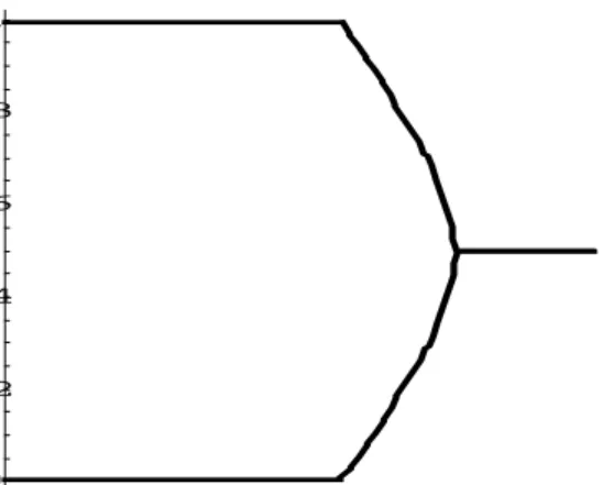
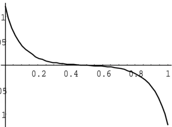
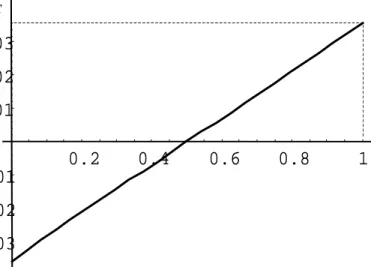
The model exhibits a smooth ’supercritical pitchfork bifurcation’. This is illustrated in Fig. 2– 5 which depict the utility differential (10) for different levels of trade costs and for the parameter values σ = 6 and α = 0.3. The corresponding bifurcation diagram is provided in Fig. 1. In our benchmark case, we findτb = 1.454, andτf = 1.337. Figs. 3 and

4 show that an agglomeration rent ΩC _{accrues to mobile entrepreneurs in a core periphery}

equilibrium. This is the positive differential VK −VK∗ which obtains for low trade costs at

λ = 1. An analytic expression of this agglomeration rent is provided in equation (A.3) in the appendix. Clearly, no such agglomeration rent obtains at intermediate equilibria since these are characterised by a utility differential of zero.

4

Taxes and tax competition

4.1

Taxes and the government objective function

We now turn to the analysis of taxes and tax competition. For simplicity we normalise the endowments of factors such thatK =K∗ _{= 1, and hence,K}

W = 2, andρ=ρ∗ = 1. Under

these assumptions, the international utility differential of the mobile factor is given by

VK −VK∗ = Ω (λ,·)−(t−t∗) (11)

where Ω (λ,·) is as defined in (10).

Note that Ω(λ,·) does not depend on tax rates. Hence, equilibria can be studied by superimposing Ω (λ,·) with the tax differentialt−t∗_{. For the case of partial agglomeration,}

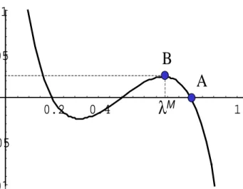
this is depicted in Fig. 6. The figure shows that there may in general be multiple stable equilibria, for instance, in the situation shown, there are two stable equilibria, one at A where home is the partial core and one at B where foreign is the partial core. To deal with this multiplicity issue, we will assume that one of the countries is originally the core (or the partial core), and the mobile factor owners cannot coordinate on moving to the other country; hence, the core region will remain the core as long as this is an equilibrium.

[Fig. 6 about here.]

To endogenise tax rates we adopt the simple reduced form government objective func-tion of Baldwin and Krugman (2004) in its quadratic form:9

W =G− t 2

2, where G= 2tλ. (12) Tax proceeds (G) enter the objective function linearly and taxes (t) are assumed to involve a quadratic loss. Since this paper is not concerned with political economy issues, this objective function is chosen on the grounds that it renders the analysis simple and tractable. Moreover as explained in detail in Baldwin and Krugman (2004, 13 f.), this objective function can be thought of as a reduced form function representing either a government which acts benevolently (i.e. it cares for the tax proceeds in order to provide public goods which raise consumers welfare) or a ‘Leviathan’ government (i.e. one which

maximises the size of the state or its own utility). It should be noted, though, that this objective function implies that governments care about agglomeration only insofar as the tax base is concerned. Other agglomeration benefits, in particular, the lower consumer price index, are not taken into account by the government.

We now turn to the analysis of tax competition in this model. Three cases have to be considered, first the dispersed equilibrium, second the CP outcome with full agglomeration, and third, the equilibrium with partial agglomeration. Note that these equilibria refer to the no-tax scenario, and it remains to be shown whether tax competition may change the outcome, say, from full to partial agglomeration.

In the first case, trade costs are so high that the only stable equilibrium is one where an equal proportion of firms locates in both countries. This case is, however, analogous to the basic tax competition model, since any small tax differential leads to a small relocation of the mobile factor. Therefore, we follow Baldwin and Krugman (2004) and turn directly to equilibria with industry agglomerated in one country.

4.2

The tax game around core-periphery equilibria

In this section we assume that trade costs are so low that industrial activity is already completely agglomerated in the domestic economy – the cases depicted in figs. 3 and 4. We follow Baldwin and Krugman (2004) in modelling the choice of taxes as a three-stage game: in the first step, the domestic government (the core) choosest, in the second step the foreign government (the periphery) chooses t∗ _{and in the third step, the market allocation}

is realised as described in the last sections. As in the analysis of Baldwin and Krugman (2004), the resulting Nash equilibrium of a tax game is a subgame perfect equilibrium, or, in their parlance, a limit-tax Stackelberg-type equilibrium.

The bifurcation type encountered in the present model, a supercritical pitchfork bifur-cation, complicates the analysis of the tax game around a core-periphery equilibrium as compared to the analysis in Baldwin and Krugman (2004). Intuitively speaking, with a supercritical pitchfork bifurcation, the utility differential (eq. (10) in our model) goes from convex to concave as the share of the mobile factor (λ) rises from below to above one half. This is illustrated by Figs. 2–5. The model used by Baldwin and Krugman, on the other hand, exhibits a subcritical pitchfork involving agglomeration forces such that the utility

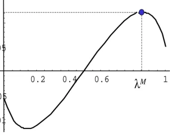
differential goes from concave to convex as λ rises from below to above one half.10 _The crucial difference between the two cases is, that, for low trade costs, the utility differential always achieves its maximum at λ = 1 in what we shall call the ‘Baldwin-Krugman case’, whereas it may achieve its maximum below values of λ = 1 in the present model. This is illustrated by fig. 4. To clarify the implications for the tax game, we divide the following analysis into two subsections, one which follows the case of Baldwin and Krugman (2004) and one which takes up the general case.

4.2.1 The Baldwin-Krugman case

We begin by assuming that trade costs are so low that the utility differential Ω achieves its maximum at λ = 1, i.e. the case depicted in fig. 3. In choosing its tax rate t, the domestic government is aware of the fact that the foreign government is able to choose a ‘delocation’ tax ratet∗

d just so low, that, for a given domestic tax ratet the tax differential

exceeds the agglomeration rent, i.e. that

ΩC _≤t−t∗

d, (13)

so that the manufacturing industry would delocate to the foreign economy. By choosing its own tax rate low enough, the domestic government may act like a limit pricing monopolist and make it unattractive for the foreign country to choose t∗

d. Let the domestic tax rate

which ensures that the foreign government cannot increase its welfare by choosing the delocation tax rate be denoted t =te. If the domestic government chooses this tax rate,

it will be in the best interest of the foreign government to accept that it is the periphery. Hence, the foreign government will choose its unconstrained tax ratet∗

uwhich maximises the

foreign government objective, taken the domestic tax rate and the fact that the domestic economy is the core as given. In this case the foreign welfare is given by

W∗_| λ=1= G∗|λ=1− (t∗₎2 2 =− (t∗₎2 2 (14)

which is obviously maximised at t∗ _{= 0. The corresponding foreign welfare level is given}

by

W∗

u = W∗|λ=1,t∗

u = 0 (15)

10_{This is elaborated on in Puga (1999, 324) and in Pfl¨uger (2004). See Fujita et al. (1999) for an}

If, on the other hand, the foreign government choosest∗

d to attract the core, foreign welfare

is given by W∗ d = W∗|λ=0,t∗ d = 2t ∗ d− ¡ t∗ d ¢₂ 2 . (16)

Hence, by equating the welfare levels W∗

u from (15) withWd∗ from (16), one obtains:

t∗

d= 0. (17)

Using te andt∗din (13) and solving with equality, the limit tax rate chosen by the domestic

government te is then given by:

te = ΩC. (18)

It remains to be checked that the core’s unconstrained tax rate is not lower than te.

Maximising (12) with respect to t, using λ = 1, yields an unconstrained tax rate of 2. Therefore, as long as te < 2, the tax equilibrium is given by the domestic government

choosing te and the foreign government choosing t∗u. In our numerical simulations, the

condition te <2 is always fulfilled.

Since the delocation tax rate and the unconstrained tax rate of the foreign government coincide, the domestic government is able to fully exploit the agglomeration rent. This difference compared to the result obtained in Baldwin and Krugman (2004) is due to the fact that, in the present analysis, taxes are levied on the mobile factor only. This sets a floor of zero for the delocation tax rate. However, the qualitative behaviour of the tax differential is the same as in Baldwin and Krugman, namely a bell-shaped curve as trade costs fall. This is illustrated in Fig. 7.11 _{In our model, this bell-shaped behaviour mimics} the evolution of the agglomeration rent as trade costs fall.

[Figs. 7 and 8 about here.] 4.2.2 The general case

Now we turn to the general case which allows for the possibility that the utility differential (10) achieves its maximum at a level λ ≤ 1. A case where λ < 1 is illustrated in Fig. 4 where the maximum utility differential is indicated by ΩM _{at λ}M_.12 _{Suppose now that we}

11_{Note that the figure contains the ‘general’ case presented in the next section as well.}

12_{The values of Ω}M _andλM _{can be easily derived analytically, but the expressions are rather messy and}

are in the core-periphery equilibrium. In contrast to the Baldwin-Krugman case, a tax differential exceeding the agglomeration rent ΩC _{will now only involve a discrete relocation}

to the foreign country if the tax differential just exceeds ΩM_{. In this case, all industry}

would move to the foreign country. For the domestic government this opens the possibility that its welfare may be increased by trading off a small tax differential in excess of the agglomeration rent with a partial loss of firms. This, however, implies that in determining the equilibrium of the tax game we cannot imposeλ= 1, contrary to the Baldwin-Krugman case. Rather, the equilibrium of the tax game will determine the domestic and the foreign tax rate and the shares of entrepreneurs in the two countries simultaneously.

The determination of this equilibrium gets more involved than in the Baldwin-Krugman case. However, the fundamental limit-tax reasoning can still be applied. In particular, the foreign government should not be able to increase its welfare by choosing a delocation tax rate so low that the industry shifts to the foreign country. This gives the following condition: W∗(t∗_d, te) = W∗ ¡ t∗_p, te ¢ (19) ⇔ 2¡ΩM _−t e ¢ −¡ΩM _−t e ¢₂ /2 = [Ω (λ)−te] 2 (1−λ)−[Ω (λ)−te]2/2,

use having been made of λ = 0 on the LHS of (19). If the domestic government chooses its limit taxte in the first step, it will not be in the best interest of the foreign government

to choose its delocation tax rate. Rather, it is then in the best interest of the foreign government to determine its optimal tax rate ,t∗

p, such that the allocation of entrepreneurs

is determined by

Ω (λ)−¡te−t∗p ¢

= 0. (20)

The optimal tax rate is found from the first order condition:

dW∗ dt∗ = 2(1−λ)−2t ∗_λ t∗−t∗ = 0⇔t∗_p = 2 (1−λ) 1 + 2λt∗, (21) where λ∗_t =−λt=− 1 Ωλ . (22)

Eqs. (19) and (20) are a system of equations which can be simultaneously solved first for te and λ and then fort∗p, and, hence, the tax differential. Again, we have to check that

the home government cannot increase its utility by setting a tax rate lower than te, which

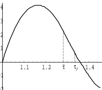
All simplifications of the model notwithstanding, it is not possible to obtain closed-form solutions. Therefore, we have to turn to numerical simulations to illustrate the tax equilibrium. We use the parameter values α= 0.3, σ = 6. We then find the level of trade costs at which λM _{= 1, so that for lower trade costs we are in the B-K case and for higher}

costs in the ‘general case’. This gives a level of trade costs, ˜τ = 1.28. Solving for the equilibrium tax rates produces the equilibrium tax gap shown in Fig. 7. The fraction of the mobile factor in the home country is shown as a function of trade costs in fig. 8.

4.3

The tax game around stable locational equilibria with partial

agglomeration

Given our characterisation of the tax equilibrium for the general case in the previous section it is now easy to characterise the tax game around stable location equilibria with partial agglomeration, say in the domestic country, a case depicted by point A in fig. 5.

We continue to model the tax game as a sequential Stackelberg game. It might appear more natural to model this game as a simultaneous Cournot-Nash game as employed in the ‘basic tax competition model’. However, it turns out that, in general, pure strategy Nash equilibria do not exist in this game (see Appendix B for details). Moreover, the use of the Stackelberg game makes our paper more easily comparable to Baldwin and Krugman (2004).

The determination of the equilibrium tax rates involves the same reasoning as previ-ously, where the choice of the delocation tax rate by the foreign government will not involve a shift of all industry to the foreign country but a shift that is limited to a locational equi-librium such as B (with corresponding λB) in fig. 5. With this modification, the system

of equations determining the two tax rates and the equilibrium share of entrepreneurs in the domestic economy is given by

W∗_(t∗ d, te) = W∗ ¡ t∗ p, te ¢ (23) ⇔¡ΩM _−t e ¢ 2 (1−λB)− ¡ ΩM _−t e ¢₂ 2 = (Ω (λ)−te) 2 (1−λ)− (Ω (λ)−te)2 2 (24) Ω (λ)−¡te−t∗p ¢ = 0 where t∗ p = 2 (1−λ) 1 + 2λ∗ t . (25)

As before, we have to check that the home government’s optimal tax rate is not lower than te, which is always satisfied in our simulations.

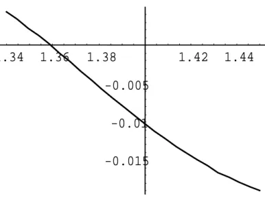
Again we have to rely on numerical simulations to obtain solutions for the equilibrium tax rates and the equilibrium allocation of entrepreneurs between the two countries. We then numerically solve the game as just described. The resulting tax differential,te−t∗(te),

is shown as function of trade costs in fig. 9. The figure shows that as trade costs increase, over the range where partial agglomeration is stable, the tax differential falls, and in fact, for sufficiently large trade costs, the tax differential becomes negative. This concurs with intuition in the sense that lowering trade costs increases agglomeration forces and therefore provides a higher shield to the partial core country. As shown in fig. 10, the share of the mobile factor in the partial core decreases with trade costs as well. It is also easily seen that for φ=φb, the equilibrium converges to the Stackelberg equilibrium presented in the

previous subsection. The tax gap over the range of trade costs τ ∈[1, τb], is shown in Fig.

11.

[Figs. 9, 10 and 11 about here.]

5

Conclusion

In this paper we have reconsidered the analysis of tax competition under agglomeration forces. Whereas the previous literature has considered either symmetric equilibria or loca-tion equilibria with complete agglomeraloca-tion, we have presented a model which also allows for partial agglomeration. We have shown that in the case with partial agglomeration, the partial core can maintain a positive tax gap even though no agglomeration rent accrues to the mobile factor. An interesting difference to Baldwin and Krugman’s analysis is that with our specification, the equilibrium for the core-periphery outcome has to be modified. In particular, it may be that over some range, partial agglomeration is the outcome of the tax game even though complete agglomeration is the only stable equilibrium without taxes.

To sum up, in a model with agglomeration forces, at very high trade costs, factor mobility implies that tax competition has much the same flavour as in the standard model. The main difference between our model and that of Baldwin and Krugman (2004) and others is the case of partial agglomeration in addition to the ‘extreme’ outcome of complete agglomeration. Our paper has shown that agglomeration forces may provide a tax shield in less extreme scenarios as well. Thus, the message of Baldwin and Krugman’s (2002) paper

and their interpretation of tax competition in Europe may carry over to the arguably more realistic scenario of partial agglomeration.

Appendix A

A full characterisation of the model is provided in Pfl¨uger (2004). For convenience, we provide some of its most important features in this appendix.

Equilibrium Once R is derived from (9), the firm scale Xi follows from (8) and the

other endogenous variables can be derived in a straightforward way. The X sector em-ploys NcXi = NR(σ−1) units of labor which we assume to be less than L in order to

ensure that both sectors are active after trade. This implies the parameter restriction

α < ρσ/(2ρ+ 1) (σ−1).

Bifurcation point The bifurcation point, i.e. the level of trade costs at which asym-metric equilibria with partial agglomeration emerge can be obtained by first calculating Ωλ, the derivative of (10) with respect toλ, then evaluating this expression around a

sym-metric equilibrium (yielding Ωs

λ) and finally by equating the resulting expression to zero

and solving for φ. Using ε≡(1−φ) gives the following intermediate steps: Ωλ = αε{ε2_{[(1−σ+λ(2 + 3σε+ 4φ))−λ}2_{(2 + 3ε+ 4φ)] + [(3σ−2)φ+φ}2_{+ 2 (σ−1)φ}3_]} (σ−1)σ(1−λε)2(λε+φ)2 . (A.1) Ωs_λ ≡ Ωλ|_λ=1/2 = 4α(1−φ) [2−4φ+σ(5φ−1)] (σ−1)σ(1 +φ)2 . (A.2) At most five equilibria Using the techniques of Robert-Nicoud (2003), it can be shown that the model has at most five equilibria (including the C-P outcomes). Moreover, it can be shown that the level of trade costs where the bifurcation fork emerges is higher than the level where full agglomeration obtains.

No black hole condition As in the CP model we want to rule out that the agglomerative forces are so strong that the symmetric equilibrium is unstable even at high (infinite) trade

costs (Fujita et al., 1999). In the present model this ‘no-black-hole-condition’ commands:

σ/(σ−1)<2ρ orσ >2.

Agglomeration rent The agglomeration rent is the positive differentialVK−V_K∗ which

obtains for low trade costs from (10) evaluate at λ= 1: ΩC ≡ Ω|_λ=1 = α σ · 3− µ 1 φ + 2φ ¶ + 1 1−σlnφ ¸ . (A.3)

Appendix B

In a situation where stable interior equilibria exist, one might think that a more natural way to model the tax game would be a simultaneous Cournot-Nash game as employed in the ‘basic tax competition model’. However, it turns out that in general, a simultaneous Nash equilibrium may not exist. To see this, consider Fig. B.1, where we have plotted reaction functions for home and foreign, denoted byr and r∗_{, for τ = 1.35 (that is, a level}

of trade costs where in the absence of taxes there are equilibria with partial agglomeratio). As can be seen in the figure, for low home tax rates, foreign chooses tax rate, say, ˆt∗_{, which}

maximises its welfare, conditional on being the partial core. The reason is that in this range, undercutting in order to attract the core would lead to lower welfare since the delocation tax rate is too low. However, above some ˜t, foreign can profitably set its delocation tax rate and attract the core. Hence, the kink in the foreign reaction function. Since the home reaction function does not intersect the foreign reaction function, no equilibrium in pure strategies exists. Hence, we use the Stackelberg game, both to make our paper more easily comparable to Baldwin and Krugman (2004), and to circumvent the problem of equilibrium existence.

References

Andersson, F. and R. Forslid (2003). Tax competition and economic geography. Journal of Public Economic Theory 5, 279–303.

Baldwin, R. E. (2001). The core-preiphery model with forward looking expectations. Re-gional Science and Urban Economics 31, 21–49.

Baldwin, R. E., R. Forslid, P. Martin, G. I. P. Ottaviano, and F. Robert-Nicoud (2003).

Economic Geography and Public Policy. Princeton: Princeton University Press.

Baldwin, R. E. and P. Krugman (2004). Agglomeration, integration and tax harmonization.

European Economic Review 48, 1–23.

Borck, R. (2003). Tax competition and the choice of tax structure in a majority voting model. Journal of Urban Economics 54, 173–180.

Bucovetsky, S. and J. D. Wilson (1991). Tax competition with two tax instruments.

Regional Science and Urban Economics 21, 333–350.

Forslid, R. (1999). Agglomeration with human and physical capital: An analytically solv-able case. CEPR Discussion paper 2102.

Forslid, R. and G. I. P. Ottaviano (2003). An analytically solvable core-periphery model.

Journal of Economic Geography. forthcoming.

Fujita, M., P. Krugman, and A. J. Venables (1999). The Spatial Economy. Cities, Regions, and International Trade. Cambridge, Mass.: MIT Press.

Fujita, M. and J.-F. Thisse (2002). Economics of Agglomeration: Cities, Industrial Loca-tion, and Regional Growth. Cambridge: Cambridge University Press.

Grandmont, J.-M. (1988). Non-linear difference equations, bifurcations and chaos: An introduction. Lecture Notes no. 5, IMSSS Economics Lecture Note Series, Stanford, CA.

Helpman, E. (1998). The size of regions. In D. Pines, E. Sadka, and I. Zilcha (Eds.),Topics in Public Economics, pp. 33–54. Cambridge: Cambridge University Press.

Kind, H. J., K. H. M. Knarvik, and G. Schjelderup (2000). Competing for capital in a lumpy world. Journal of Public Economics 78, 253–274.

Krugman, P. (1991). Increasing returns and economic geography. Journal of Political Economy 99, 483–99.

Krugman, P. and A. J. Venables (1995). Globalization and the inequality of nations.

Quarterly Journal of Economics 60, 857–880.

Ludema, R. D. and I. Wooton (1999). Regional integration, trade and migration: Are demand linkages relevant for Europe? In R. Faini, J. de Melo, and K. F. Zimmer-mann (Eds.), Migration: The Controversies and the Evidence, pp. 51–68. Cambridge: Cambridge University Press.

Ludema, R. D. and I. Wooton (2000). Economic geography and the fiscal effects of inte-gration. Journal of International Economics 52, 331–357.

Neary, J. P. (2001). Of hype and hyperbolas: Introducing the new economic geography.

Journal of Economic Literature 39, 536–61.

Ottaviano, G. I. P. and J.-F. Thisse (2003). Agglomeration and economic geography. In J. V. Henderson and J.-F. Thisse (Eds.), Handbook of Urban and Regional Economics. Amsterdam: North-Holland. forthcoming.

Pfl¨uger, M. (2004). A simple, analytically solvable chamberlinian agglomeration model.

Regional Science and Urban Economics. forthcoming.

Puga, D. (1999). The rise and fall of regional inequalities. European Economic Review 43, 303–334.

Robert-Nicoud, F. (2003). The structure of simple ’new economic geography’ models (or, on identical twins). Mimeo, University of Geneva.

Venables, A. J. (1996). Equilibrium location of vertically linked industries. International Economic Review 37, 341–359.

Wilson, J. D. (1999). Theories of tax competition. National Tax Journal 52, 269–304. Zodrow, G. R. and P. Mieszkowski (1986). Pigou, Tiebout, property taxation and the

1 1.1 1.2 1.3 1.4 1.5 1.6 0 0.2 0.4 0.6 0.8 1 λ τ

0.2

0.4

0.6

0.8

1

-0.1

-0.05

0.05

0.1

λ

0.2

0.4

0.6

0.8

1

λ

-0.03

-0.02

-0.01

0.01

0.02

0.03

Ω

0.2

0.4

0.6

1

-0.01

-0.005

0.005

λ

λ

Ω

0.2

0.4

1

-0.01

-0.005

0.005

0.01

Ω

λ

λ

A

B

0.2

0.4

0.6

0.8

1

-0.0075

-0.005

-0.0025

0.0025

0.005

0.0075

Ω

(

λ

)

λ

t-t*

A

B

1.1

1.2

τ

0.01

0.02

0.03

0.04

t

t*

τ

~

1.05 1.1 1.15 1.2 1.25 1.3

τ

λ

1.34

1.36

1.38

1.42

1.44

-0.015

-0.01

-0.005

t

-t*

τ

1.34

1.36

1.38

1.42

1.44

τ

0.88

0.89

0.91

0.92

0.93

0.94

λ

1.1

1.2

1.4

τ

-0.02

-0.01

0.01

0.02

0.03

0.04

t

_-

_t

τ

τ

0.006 0.008 0.012 0.001 0.002 0.003 0.004 0.005 r* r t* t