ORIGINAL ARTICLE
Ensemble of texture descriptors and classifiers for
face recognition
Alessandra Lumini
a, Loris Nanni
b,*, Sheryl Brahnam
c aDISI, Universita` di Bologna, Via Venezia 52, 47521 Cesena, Italy bDEI, University of Padua, viale Gradenigo 6, Padua, Italy c
Computer Information Systems, Missouri State University, 901 S. National, Springfield, MO 65804, USA
Received 18 November 2015; revised 22 March 2016; accepted 12 April 2016 Available online 21 April 2016
KEYWORDS
Face recognition; Similarity metric learning; Ensemble of descriptors; Support vector machine
Abstract Presented in this paper is a novel system for face recognition that works well in the wild and that is based on ensembles of descriptors that utilize different preprocessing techniques. The power of our proposed approach is demonstrated on two datasets: the FERET dataset and the Labeled Faces in the Wild (LFW) dataset. In the FERET datasets, where the aim is identification, we use the angle distance. In the LFW dataset, where the aim is to verify a given match, we use the Support Vector Machine and Similarity Metric Learning. Our proposed system performs well on both datasets, obtaining, to the best of our knowledge, one of the highest performance rates pub-lished in the literature on the FERET datasets. Particularly noteworthy is the fact that these good results on both datasets are obtained without using additional training patterns. The MATLAB source of our best ensemble approach will be freely available at https://www.dei.unipd.it/node/ 2357.
Ó2016 The Authors. Production and hosting by Elsevier B.V. on behalf of King Saud University. This is an open access article under the CC BY-NC-ND license (http://creativecommons.org/licenses/by-nc-nd/4.0/).
1. Introduction
Face recognition has been an area of intense study since the 1960s. Innovative applications making use of this technology are continuously being developed at a rapid pace.
Contempo-rary face recognition applications can be divided into three areas that depend on the goal of the face recognition task: (1) face verification, where the goal is to authenticate the iden-tity of a face image with a corresponding template; (2) face identification, where the goal is to find a match in a database of face images; and (3) face tagging (a relatively new variation of face identification), where the goal is to label face images based on identification when matched. Face recognition is now an essential component in biometric security, access man-agement, criminal identification, and image sorting and retrieval.
The main goal of face recognition is to compare two images of faces and solve the problem of determining whether both images are of the same person or of two differ-ent people. This problem is difficult because two images of
* Corresponding author.
E-mail addresses: [email protected] (A. Lumini), loris. [email protected] (L. Nanni), [email protected] (S. Brah-nam).
Peer review under responsibility of King Saud University.
Production and hosting by Elsevier Applied Computing and Informatics (2017)13, 79–91
Saudi Computer Society, King Saud University
Applied Computing and Informatics
(http://computer.org.sa)
www.ksu.edu.sa www.sciencedirect.com
http://dx.doi.org/10.1016/j.aci.2016.04.001
2210-8327Ó2016 The Authors. Production and hosting by Elsevier B.V. on behalf of King Saud University. This is an open access article under the CC BY-NC-ND license (http://creativecommons.org/licenses/by-nc-nd/4.0/).
the same person can vary considerably in time, pose, facial expression, illumination conditions, occlusions, and image quality. Most state-of-the-art face recognition techniques per-form well when facial images are captured in optimal (labo-ratory) conditions where lighting is controlled and samples provide full frontal views, but when facial images are cap-tured in the wild – where pose, age, and facial expressions change and where environmental conditions such as lighting are less than ideal – performance deteriorates. The difficulty lies in teasing out the specific features indicative of identity from the mass of features expressing other conditions. Even the best classifier will fail if an insufficient number of features indicative of identity are isolated. One way to tackle this problem is to usemultibiometrics, which recognizes individu-als via biometric fusion [1], whether multimodal, multi-instance, multisensorial[2], or multialgorithmic. Of particular importance to both single trait biometrics and multibiomet-rics is the identification of face descriptors that are discrimi-native yet insensitive to information having nothing to do with identity, such as pose variations, changes in facial expression, and lighting conditions.
Some of the most notable face recognition techniques devel-oped the last five decades [3] include Principal Component Analysis, Elastic Template Matching, Discriminant Analysis, Local Binary Patterns (LBPs), Algebraic moments, Gabor Fil-tering[4], and Neural Networks[5]. One way to categorize face recognition techniques is to look at how a face is represented
[3].Appearance based approachesutilize global texture features such as Eigenfaces[6]or some other linear transformation. In addition to the information found in the texture of a face image,Model based approaches take into account the shape of the face, whether 2D[7]or 3D.Geometry or template based approaches compare an input image with a set of templates constructed using either statistical tools or by analyzing local facial features and their geometric relationships [8]. Neural Networksinclude approaches based on ‘‘deep learning”where the representation of faces is learned during the training pro-cess [5]. This last class includes approaches that are often referred to as ‘‘deep methods”in opposition to ‘‘shallow meth-ods,”and differs from a second class of approaches where the representation of the face image is derived from ‘‘handcrafted” image descriptors.
Recent developments in the first class of shallow methods include the work of Pinto et al.[9]who describe a set of V1-like features that are composed of a population of Gabor fil-ters. V1-like features are insensitive to view, lighting, and many other image variations. The feature sets proposed by Cao et al.
[10]that encode the local micro-structures of a face into a set of more uniformly distributed discrete codes are excellent examples of a good tradeoff between discriminative power and invariance, as are Patterns of Oriented Edge Magnitudes (POEM), a feature set proposed in[11,12]. POEM is an ori-ented spatial multiresolution descriptor that captures informa-tion about the self-similarity structure of an image. Some feature sets that work well in the wild include those described in[13]and more recently in[14], where monogenic binary cod-ing (MBC) is presented. MBC decomposes an original signal into three components (amplitude, orientation, and phase) that encode local variation. A histogram is then extracted from the local features. This efficient descriptor significantly lowers the time and space complexity compared with other Gabor-transformation-based local feature methods.
Another approach for overcoming variations in pose and illumination is to combine texture-based descriptors with other techniques. For example, in[15]an accurate 3D shape model works by mapping images that vary in pose to a full frontal view. Discriminative models capable of handling aging, facial expressions, low light, and over-exposure are then obtained by comparing billions of faces. One approach described in
[16] trains binary classifiers on sixty-five describable visual traits that were manually labeled on the training set. Another approach based on ‘‘simile classifiers”removes the need for a manually labeled training set by training the binary classifiers to recognize the similarity of faces (using the whole image and patches) to specific reference people. Both approaches exploit the power of simple low-level features (such as image intensi-ties in RGB and HSV color spaces, edge magnitudes, and gra-dient directions). A drawback of these approaches, however, is that they required using affine warping to obtain pose invari-ance. In[17]an identity-preserving alignment is proposed. In this approach, face warping reduces differences in poses and expressions while preserving differences indicative of identity. Binary classifiers are trained both to perform an ‘‘identity-pre serving”alignment and to recognize people.
The Multi-scale Local Phase Quantization (MLPQ) method proposed in[18]is a blur-robust image descriptor. MLPQ is computed regionally and adopts a component-based framework to maximize the insensitivity to misalignment, a phenomenon frequently encountered in blurring. Regional features are bined using kernel fusion. The MLPQ representation is com-bined with the Multiscale Local Binary Pattern (MLBP) descriptor according to a supervised fusion that is based on Ker-nel Discriminant Analysis (KDA). This step is necessary to increase insensitivity to illumination. It should be pointed out here, however, that the MLPQ representation in [18] was obtained using a supervised transform and a different testing protocol. Thus, the results reported in[18]on the LFW dataset are not comparable with the approach proposed in this paper.
A real breakthrough in the field of face recognition was the introduction of ‘‘deep methods,”which are based on the appli-cation of deep learning to this pattern recognition problem. The first interesting paper in this area was[5], where a convo-lutional neural network (CNN) was employed to learn a metric between face images. This was a precursor to the recent highly successful application of CNNs to face verification. So power-ful is the deep learning approach that after a decade of study researchers[19]have recently announced that we are now able to close the ‘‘gap to human-level performance in face verifica-tion.”With an approach based on a 3D model for face align-ment and an ensemble of CNNs to find a numerical description of the forward-looking face, DeepFace has achieved 97.25% accuracy on the LFW dataset, which is very close to the human level accuracy of 97.53% in face verification. Another work [20] that is based on Gaussian Processes and multi-source training sets has achieved 98.52% accuracy on the LFW dataset, which is better than human performance.
Many deep learning approaches [21–23] have also signifi-cantly outperformed previous systems based on low level features in face recognition. There are two innovations of note in these deep learning approaches based on low-level features. The first is in face identification, thanks to the last hidden layer, which contains features highly discriminative in performing large-scale face identification. The second is in both face identification and verification, thanks to supervising
deep neural networks that minimize the distance between fea-tures of the same identity while simultaneously decreasing intra-personal variations.
Although one of the best benchmarks in face recognition is the LWF dataset, there are some limitations of this dataset that need some remarks: in particular the limitations discussed in[24], which investigated the availability of a big training set and its impact on recognition performance. During the history of the LFW benchmark, the largest improvements have been obtained the last few years by applying deep learning tech-niques to huge datasets containing outside labeled data. The amount of training data expanded a hundred times from 2010 to 2014, i.e., from about ten thousand training samples in [25]to four million images in [19]. The best performance using a training set of less than 10,000 images with deep learn-ing was lower than 85%. Accordlearn-ing to the study in[24], the performance on large databases of faces seems to rise linearly as data size increases, but a long-tail effect emerges when the number of individuals becomes greater than 10,000. Increasing individuals (with a few instances per person) does not help to improve performance. Moreover, it is worth noting that the Megvii Face Recognition System [24], which achieves 99.50% accuracy on the LFW, did not reach acceptable per-formance in real-world security certification scenarios that contend with a high range of age variation, proving that there is still a real gap between machine recognition and human per-formance. The main drawback of these methods is that they require millions of images for training. As a consequence their results on benchmarks are not directly comparable with approaches obtained using a testing protocol based on a few training samples.
The approach presented in this paper can be referred to as
shallow, since unlike deep methods, our proposed approach is based on a representation of the face image using handcrafted local image descriptors. The system presented here is based on preliminary results reported in[26]that demonstrate how the performance of the POEM descriptor[12](one of the most effi-cient and one of the highest performing descriptors recently proposed in the literature) can be enhanced with an ensemble of classifiers that combine different preprocessing techniques that vary a set of feature extraction parameters. However, here we also test our proposed system using a set of ‘‘learned” fea-tures, which have been obtained from the internal representa-tion of a deep method, especifically a Convolurepresenta-tional Neural Network (CNN) trained for the face recognition problem. We want to underscore that the use of ‘‘learned features”does not put the proposed approach in the category of a ‘‘deep method”approach since the training of the classifier is per-formed in a traditional, shallow way.
The key additions to[26], on which the approach proposed in this paper is based, are the following:
The combination of several feature extractors using differ-ent enhancemdiffer-ent techniques.
The improved performance obtained using two different classifiers for face verification: Support Vector Machines (SVMs) and Similarity Metric Learning1(SML)[25].
The utilization of the method proposed in[27]2for
synthe-sizing a single frontal face view starting from an uncon-strained photo (useful because LFW images are unconstrained).
The combination of ‘‘learned”and ‘‘handcrafted”features. The resulting fusion based solely on the handcrafted fea-tures obtains, to the best of our knowledge, one of the highest mean accuracy ratings on the FERET datasets published in the literature. Moreover, the fusion produces very good results on the LFW dataset. The ensemble based on the fusion of learned and handcrafted features improves performance on both the FERET and LFW datasets even further.
It is important to point out that we have used the same parameters for both the FERET and the LFW datasets to avoid any overfitting (in the literature a number of papers report varying the parameters that are used in the two datasets, thereby increasing the likelihood of overfitting the given method to that dataset).
2. The proposed approach
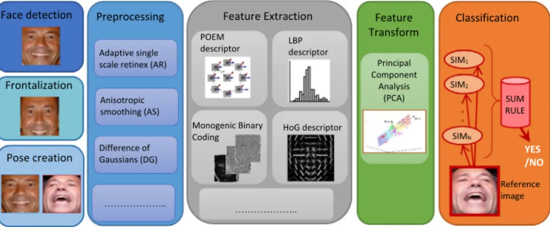
The main idea of the proposed approach is to design an ensem-ble of classifiers trained on different descriptors extracted from the face image. Moreover, in order to perturb the information given to the base classifiers and to make the ensemble stronger, we designed several perturbations at different steps in the clas-sification process: in the image preprocessing, feature transfor-mation, and matching steps. The general schema of the complete approach is illustrated in Fig. 1. Detailed descrip-tions of the methods used in each step are provided below in this section.
As illustrated inFig. 1, the proposed approach can be bro-ken down into the following steps:
Face detection:first the precise position of the face image is detected as in[27], and the resulting face is cropped and aligned according to eye position.
Frontalization:the approach proposed in[27]is used to syn-thesize frontal views of faces from the detected face (this step is useful in making the feature representation indepen-dent of pose changes).
Pose creation:to tackle pose variation, we make use of three additional poses obtained by vertically flipping the image. In other words, we train four classifiers: the first using the original images for the two faces to be matched; the second using the vertical flip of the second face; the third using the vertical flip for the first image; and the fourth using the ver-tical flip for both images. The four systems are then simply combined by sum rule.
Preprocessing:several enhancing methods have been tested in this work in order to make the feature extraction more robust to changes in illumination, noise, etc. The parallel use of different approaches is performed as a perturbation strategy in order to obtain diversity among the classifiers. The input of this step is the frontalized image, and the out-put is a set of images preprocessed according the following approaches: Adaptive single scale retinex[28], Anisotropic smoothing[29], Difference of Gaussians[30], an approach
1
Code:
based on the low-frequency discrete cosine transform[31], Oriented Local Histogram Equalization [32], Multi-Scale Retinex [33], Isotropic Smoothing Normalization [34,35], and Gradientfaces[36].
Feature extraction:this step is performed separately on each image resulting from the previous preprocessing method in order to obtain different descriptors from each image. The descriptors extracted include the following: Local Binary Patterns (LBPs)[37], Histogram of Gradients[38], POEM
[11], Heterogeneous Auto-Similarities of Characteristics (HASC) [39], Gaussian of Local Descriptors (GOLD)
[40], and Monogenic Binary Coding[14].
Feature transformation:before classification the dimension-ality of each descriptor is reduced via Principal Component Analysis (PCA)[41].
Classification:a set of general-purpose classifiers is trained on each reduced descriptor. The final decision is then deter-mined according to the sum rule by summing up the scores/ similarity values (SIMi) obtained from each classifier. In
this work, the simple angle distance is used in the FERET datasets, where the aim is identification. Linear SVMs[42]
and SML [25] are used on the LFW dataset, where the aim is to verify a given match.
2.1. Hard Frontalization (HF)
Unlike other frontalization methods that transform a 3D facial model to fit a particular facial appearance, HF, proposed in
[27], uses single 3D reference geometry to synthesize frontal views of faces from different facial poses captured in the wild. This idea is based on the observation that for frontalization a rough approximation to a single 3D facial shape is, for all practical purposes, as good as any other, including a more individualized construction of a 3D structure.
The HF process begins by utilizing standard facial feature detectors to detect and crop a face when found in an image. This cropped image is rescaled to a standard coordinate sys-tem, where a set of 49 facial features are used to render a gen-eric 3D model. A 34 projection matrix is then estimated from the 2D query coordinates and the corresponding 3D model coordinates. This matrix is used to back-project the query intensities (facial colors) to the reference coordinate system, which are then overlaid on the frontalized model.
Intensities are borrowed from corresponding symmetric parts of the face to fill in missing areas in the generic 3D model for a final result.
HF requires four steps: (i) the pose estimation process, which is based on a synthetic rendered view of a texture 3D model by means on a rotation matrix and a translation vector; (ii) frontal pose synthesis using bi-linear interpolation to sam-ple the intensities of the initial frontalized view produced by back projecting the query features onto the reference coordi-nate system of the 3D model; (iii) visibility estimation, which is performed using a variation of the multiview 3D reconstruc-tion method where an approximareconstruc-tion to the 3D reference face and a single view (rather than multiple views) is employed to estimate visibility; and (iv) detection of problems introduced by conditional soft-symmetry using a standard representation (LBP) and a classifier (SVM) to take advantage of the fact that regardless of the actual shape of the face the same image region in the frontal face always corresponds to the same areas.
2.2. Preprocessing techniques
Before the feature extraction step, it is possible to address the problem of illumination variation by using some recently developed image enhancement techniques:
Adaptive single scale retinex (AR)[28]: a variant of the reti-nex technique, this approach was originally developed to improve scene detail and color reproduction in the darker areas of an image. This technique normalizes illumination using the spatial information between surrounding pixels (it should be noted that AR produced the best results in our experiments).
Anisotropic smoothing (AS)[29]: a simple automatic image-processing normalization algorithm, AS begins by estimat-ing the illumination field and then compensates for it by enhancing the local contrast of the image in a fashion sim-ilar to human visual perception. This technique has proven highly effective with standard face recognition algorithms across many face databases[29].
Difference of Gaussians (DG):this is a normalization tech-nique that relies on the difference of Gaussians to produce a normalized image. A band-pass filter is applied to an input image before the feature extraction step. In our experi-ments, the log transform is used before filtering as in[30].
Low-frequency discrete cosine transform (DCT) based approach[31]: this is an illumination normalization approach for face recognition, where a discrete cosine transform (DCT) is employed to compensate for illumination variations in the logarithm domain. The rationale is that since illumination variations mainly lie in the low-frequency band, an appropri-ate number of DCT coefficients are truncappropri-ated to minimize variations under different lighting conditions.
Oriented Local Histogram Equalization (OLHE)[32]: this is a histogram equalization that compensates illumination while encoding rich information on the edge orientations.
Multi Scale Retinex (MSR)[33]: this is a multiscale retinex (a model of the lightness and color perception of human vision) that achieves simultaneous dynamic range compres-sion, color consistency, and lightness rendition with the aim of improving fidelity of color images to human observation.
Isotropic Smoothing Normalization (ISN)[34]: this method deals with the problem of face verification across illumina-tion by means of isotropic smoothing normalizaillumina-tion (a dif-fusion step which basically updates each pixel using an average of its neighboring pixels, regardless of the image content surrounding the region under consideration).
Photometric Normalization (PN)[35]: this is a robust illu-mination normalization which operates as a simple and effi-cient preprocessing chain based on gamma correction, difference of Gaussian filtering, masking and contrast equalization, and photometric normalization, which elimi-nates most of the effects of changing illumination while still preserving the essential appearance details that are needed for recognition.
Gradientfaces (GFs) [36]: this is not properly an enhance-ment method but rather an illumination insensitive measure derived from the image gradient that is robust to illumination changes, including those in uncontrolled natural lighting envi-ronments. In this work we use Gradientfaces as a preprocess-ing approach to represent an image in the gradient domain.
2.3. Feature extraction
The feature extraction step is performed on each preprocessed image as detailed in the previous step in order to extract the following descriptors: LBP, HoG, POEM, MBC, HASC, GOLD, RICLBP, and CLBP. Each of these feature extraction methods is discussed below.
2.3.1. Local Binary Patterns (LBPs)
LBP[37]is a gray scale local texture operator with powerful discrimination and low computational complexity. Among LBPs many desirable properties are its invariant to monotonic grayscale transformation; hence, it has low sensitivity to changes in illumination.
The LBP operator represents the difference between a pixel
xand its symmetric neighbor set ofPpixels placed on a circle radius ofR(when a neighbor does not coincide with a pixel, its value is obtained by interpolation). In this work we useP= 8 and R= 1. We also use LBP with uniform bins. The LBP descriptor is extracted from a set of subregions that are obtained by dividing each image cell into 910 equal nonoverlapping regions. The set of descriptors are concate-nated for describing the entire image.
2.3.2. Histogram of Gradients (HoG)
HoG [38] represents an image by a set of local histograms which count occurrences of gradient orientation in a local cell of the image. The HoG descriptor can be extracted in four steps: (i) the computation of gradients of the image, (ii) the division of the image into small subregions, (iii) the building a histogram of gradient directions for each subregion, and (iv) the normalization of histograms to achieve better invari-ance to changes in illumination or shadowing. The subregions are obtained by dividing each image cell into 88 equal nonoverlapping regions. The set of descriptors are concate-nated for describing the whole image.
2.3.3. Patterns of gradient Orientations and Magnitudes (POEM)
The POEM descriptor[11]relies on characterizing edge direc-tions of the local face appearance and its shape using the dis-tribution of local intensity gradients. It accomplishes this by measuring the edge/local shape information and the relation between the information in neighboring cells.
Extracting POEM descriptors is a three step process:
Step 1:Preform gradient computation and orientation quan-tization. This is accomplished by computing the gradient image and then by discretizing the orientation of each pixel over 0–p (for an unsigned representation) or 0–2p (for a signed representation). A soft assignment can be employed to avoid problems due to image degradation, where the original magnitude of a pixel can be decomposed into two parts and then assigned into its two nearest-neighbors ori-entation. In our experiments, we utilize the unsigned 0–p representation and soft assignment.
Step 2.Calculate the magnitude accumulation. A local his-togram of orientations is calculated considering all pixels within a local image patch (cell). As a result, each pixel car-ries information about the distribution of the edge direction of a local cell.
Step 3.Calculate self-similarity.In this step the accumulated magnitudes are encoded across different directions using the LBP-based operator within a larger patch (block). Based on previous experimental results[26], the Dense LBP (DLBP) is used in our experiments instead of standard LBP.
The result of the POEM extraction process is a set of ‘‘uni-directional”POEM maps. To incorporate spatial information, the POEM maps are divided into 88 nonoverlapping regions. Histograms are then extracted from each region. The final POEM-HS descriptor is the concatenation of all uni-directional descriptors at different orientations.
The POEM descriptor depends on a large number of parameters that need to be tuned specifically for each applica-tion. In our experiments the number of orientations dis-cretized, and the size of the cell, the size of the block, and the number of neighbors considered in LBP have been set according to[43](i.e. to 3, 7, 5, and 8, respectively).
2.3.4. Monogenic Binary Coding (MBC)
MBC[14]is an efficient texture descriptor. The monogenic sig-nal is a rotation-invariant representation that extracts the phase, amplitude, and orientation of a signal. Because it extracts multiple-orientation features without using steerable
filters, it has a much lower time and space complexity than the Gabor transformation (e.g. with time, there are three convolu-tions on each scale, and with space, there are three feature maps on each scale). Monogenic signal representation is the combination of an image and its Riesz transform. This repre-sentation decomposes an original signal into three compo-nents: amplitude, orientation, and phase. Multiresolution Monogenic Signal Representation is obtained by performing band-pass filtering on an image before applying the Riesz transforms by means of log-Gabor filters. In[14]three differ-ent resolutions are suggested that correspond to differdiffer-ent scal-ing factors of the bandwidth. Monogenic Binary Codscal-ing encodes monogenic signal features in two complementary steps: (i) the encoding of the variation between the central pixel and its surrounding pixels in a local patch (monogenic local variation) and (ii) the encoding of the value of central pixel itself (monogenic local intensity coding). A monogenic binary code (MBC) map is then calculated as the concatenation of histograms from each of the amplitude, phase, and orientation components of the monogenic signal representation[14]. Lin-ear Discriminant Analysis (LDA)[44]is used as a final step to simultaneously reduce the histogram feature dimension and enhance its discriminative power. This is accomplished in three steps: (i) the MBC feature map is partitioned into blocks, (ii) each block is further partitioned into subregions, and (iii) LDA is used in each block both to learn a projection matrix from the training set of feature maps of its subregions and to reduce dimensionality of the histogram feature.
Each step in MBC (the multiscale log-Gabor filtering, sub-region histogram computing, and feature combination by LDA) involves several parameters. In our experiments, all parameters have been set according to those in the original paper. However, in this work an unsupervised feature trans-form (PCA), as described below, is used instead of LDA. The final descriptor is composed of three feature vectors, one for each component (amplitude, orientation, and phase) of the original signal, labeled in the experimental section as MBCa, MBCo,MBCp, respectively. The three descriptors are
not fused at the feature level but rather at the score level according to the weighed sum rule: MBC = (MBCa+ MBCo+ MBCp)/3.
2.3.5. Heterogeneous Auto-Similarities of Characteristics (HASC)
HASC[39]is applied to heterogeneous dense feature maps and simultaneously encodes linear relations by covariances (COV) and nonlinear associations through information-theoretic measures, specifically entropy combined with mutual informa-tion (EMI). The basic supposiinforma-tion behind HASC is that linear relations alone are unable to capture the structural complexity of many objects. Using covariance matrices as region descrip-tors is advantageous because it is low-dimensional and robust to noise and pose changes; however, a single pixel outlier can dramatically alter results, making the descriptor highly sensi-tive to impulsive noise. Moreover, the covariance among two features is optimally able to encapsulate the features of the joint PDF only if they are linked by a linear relation. EMI overcomes these limitations. The entropy (E) of a random vari-able measures the uncertainty associated with the value of the variable, and the mutual information (MI) of two random variables captures the generic dependencies (both linear and
nonlinear). HASC takes advantage of these two properties by dividing an image into patches and creating an EMI matrix. Each diagonal entry of the EMI matrix captures the amount of uncertainty or unpredictability related to a given feature whereas off-diagonal entries capture the mutual dependency between two different features.
HASC boosts discriminative performance because the com-bination of COV with EMI captures different features of the joint underlying PDFs. Multiple experiments in [39] demon-strate that HASC is superior in performance to its individual components COV and EMI. This makes HASC a versatile descriptor for a large range of applications. HASC is extracted separately from subregions of the whole image. The subregions are obtained by dividing each image cell into 88 equal nonoverlapping regions. The set of descriptors are concate-nated for describing the entire image.
2.3.6. Gaussian of Local Descriptors (GOLDs)
GOLD[40]is a recent improvement of the well-known Bag of Word (BoW) approach [45] for extracting features from an image. The canonical BoW descriptor generates a codebook (via clustering methods on the training set) from a set of extracted local features that are then encoded into codes to form a global image representation. Instead of using a cluster-ing method, GOLD substitutes a flexible local feature repre-sentation obtained by parametric probability density estimation that does not require quantization. Quantization has the drawback of tightly tying dataset characteristics to the feature representation since quantization is learned from the training set, and the cluster centers reflect the training data distribution.
GOLD is a four-step process: (i) feature extraction, where dense SIFT descriptors are extracted on a regular grid of the input image; (ii) spatial pyramid decomposition, where the image is decomposed into subregions by a multilevel recursive image decomposition and where features are softly assigned to regions according to a local weighting approach; (iii) paramet-ric probability density estimation, where each region is repre-sented as a multivariate Gaussian distribution of the extracted local descriptors by inferring local mean and covari-ance, and (iv) projection on the tangent Euclidean space, where the final region descriptor, the covariance matrix, is pro-jected on the tangent space and concatenated to the mean.
2.3.7. Rotation Invariant Co-occurrence among adjacent LBP (RICLBP)
The original LBP does not preserve structural information among binary patterns; therefore, a set of co-occurrences among adjacent LBPs (i.e. a co-occurrence matrix among LBP pairs, or CoALBP) is extracted and converted to a CoALBP histogram feature. The rotation invariance of CoALBP is obtained by attaching a rotation invariant label to each LBP pair [46]. In this work the RICLBP descriptor has been tested using the following LBP parameters: (R= 1,
P= 8), (R= 2,P= 8) and (R= 4,P= 8).
2.3.8. Complete LBP (CLBP)
CLBP[47]is an LBP variant which utilizes both the sign and magnitude information in the difference between the central pixel and some pixels in its neighborhood (the conventional LBP operator only uses the sign component). CLBP also
con-siders the intensity of the central pixel; therefore, the final code is obtained from the combination of three codes: CLBP_S, which considers the sign component of the difference (i.e. the standard LBP), CLBP_M, which considers the magnitude component of the difference, and CLBP_C, which considers the intensity of the central pixel. In this work the CLBP descriptor has been tested using the following two LBP config-urations: (1, 8) and (2, 16).
2.4. Feature transform
We tested several approaches for dimensionality reduction in our experiments to find the best way of reducing the dimen-sionality of each descriptor before the classification step. According to[48]nearly all spectral methods provide approx-imately the same accuracy when used with the same energy cut. In our experiments, however, the best performance was obtained using PCA [41], one of the most popular methods for unsupervised dimensionality reduction. PCA maps feature vectors into a smaller number of uncorrelated directions calcu-lated to preserve the global Euclidean structure, and it also extracts an orthogonal projection matrix so that the variance of the projected vectors is maximized.
In this work we selected an orthogonal basis designed to maintain enough components to explain 99% of the input vari-ance for LBP, HASC, GOLD, HOG and Deep Features (see Section3.3) or the components where the eigenvalues are lar-ger than 10e4 for POEM and MBC[3]. When SML is used as the classifier, we retained the first 300 components, as sug-gested in[26].
2.5. Classification
In the classification step, each preprocessed image together with its extracted descriptor induces a different individual clas-sifier or distance measure. Therefore, for each descriptor we have a different score or similarity measure SIMifor the
refer-ence image. The final decision of the ensemble is obtained by combining all the scores by sum rule. This is a straightforward method that was selected because the number of classifiers is quite high when including all the preprocessed images and all the descriptors and artificial poses under consideration in this work. Moreover, the simple sum rule does not require a deep analysis of the uncertainty space of ensemble classifiers, as was performed in[49–51].
In the FERET datasets, where the aim is identification, we use theangle distanceas the similarity function to compare two faces. The angle distance between two vectors is the size of the angle between the two directions originating from the observer and pointing toward these two vectors. It can be calculated as the angle whose cosine is the ratio between the dot product of the two vectors and the product of their magnitudes. In the LFW dataset, where the aim is to verify a given match, a gen-eral purpose binary classifier can be used to distinguish between genuine and impostor matchings. In this work we test Linear SVM[40]and SML[25].
Support Vector Machines (SVMs)[52] are a general pur-pose two-class classifier that finds the equation of a hyperplane that maximally separates all the points between the two classes. SVM handles nonlinearly separable problems using kernel functions to project the data points onto a
higher-dimensional feature space. We used different kernels in our experiments, but the best results were obtained with a linear kernel. The SVM classifier is trained to distinguish between genuine and impostor matches. Therefore, a training pattern is the combinationx of two descriptorsxiandxjand a label
l. The two descriptors are combined in order to obtain the fol-lowing resulting vector: x= (xixj)2./(xi+xj), where the element-wise power and the element-wise division (./) are performed.
Similarity Metric Learning (SML)[25]is a novel regulariza-tion framework to learn similarity metrics for unconstrained face verification where similarity metric learning over the intra-personal subspace is performed. The similarity function between the imagesxi,xjis defined as follows:
fM;Gðxi;xjÞ ¼sGðxi;xjÞ dMðxi;xjÞ
wheresGðxi;xjÞ anddMðxi;xjÞare a weighed similarity and a weighed distance, respectively. The two weigh matrices G
andMare learned from the training set such thatfM;Gðxi;xjÞ
report a score proximal to 1 ifxi,xjbelongs to the same class and a small score otherwise. The learning objective incorpo-rates the robustness to large intra-personal variations and the discrimination power of novel similarity metrics.
3. Experimental section 3.1. Datasets
Our proposed system is evaluated on the FERET [53] and LFW[54] benchmark databases. The FERET database con-tains five datasets: Fa (1196 images), Fb (1195 images), Fc (194 images), Dup1 (722 images), and Dup2 (234 images). The gallery set is Fa, and the other datasets are used for test-ing. Fb contains pictures taken on the same day as the Fa images, using the same camera and under the same lighting conditions. Fc is a dataset of pictures taken on the same day as Fa but with different cameras and under different illumina-tion condiillumina-tions. The Dup1 and Dup2 datasets contain pictures that were taken within the same year as Fa for Dup1 and later than one year for Dup2. The standard FERET evaluation pro-tocol involves comparing images in the testing sets to each image in the gallery set. In our experiments, all FERET gray scale images are aligned using the true eye positions and cropped to 110110 pixels.
The LFW [54] database contains 13,233 images of 5749 celebrities that were collected from the internet (Yahoo news). A total of 1680 faces appear in more than two images. LFW is commonly considered a very challenging dataset for face veri-fication since the faces were acquired in uncontrolled environ-ments. As a result, the images vary greatly in illumination, pose, and image quality, as well as in the age of the different celebrities. Two views are provided in the LFW database. View 1 contains a training set of 2200 face pairs and a testing set of 1000 face pairs and is used for model selection purposes only. View 2 contains 10 nonoverlapping sets of 600 matches and is for performance reporting. View 2 images can be used for 10-fold cross-validation algorithms and for testing the parameters developed on View 1. The classifiers are trained using only View 1. In this work we use preprocessed ‘‘prealigned” and ‘‘funneled”images using commercial face alignment software available on the LFW website.
The official testing protocols of both datasets are employed in the experiments reported in this section. For LFW, the
Image-Restricted/No Outside Data Resultsis used. The perfor-mance indicator is the recognition rate in the FERET datasets and accuracy in the LFW dataset. Accuracy is the proportion of true classification results (both true positives and true neg-atives) in the population.
3.2. Results
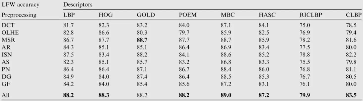
The first experiment was aimed at evaluating the different descriptors when combined with the preprocessing methods listed in Section2. The experiments were carried out on the LFW dataset using the complete approach described in
Fig. 1 (including the steps of frontalization, pose creation, and feature transformation). The classifier used in these experiments is SML. The results reported in Table 1 show
the performance of each descriptor combined with each preprocessing method, with All denoting fusion by sum rule of all the approaches in the same column.
The results inTable 1clearly show that the fusion obtained by combining all the preprocessing methods outperforms the best single preprocessing method for each given descriptor. Another interesting finding is that the best descriptor for this classification problem is MBC, and the best single preprocess-ing method is MSR.
The second experiment was aimed at evaluating the utility of some of the steps in the proposed system:
Frontalization: where [Y/N] denotes the presence/absence, respectively, of the frontalization step.
Poses: where [Y/N] denotes the presence/absence, respec-tively, of the artificial poses for LFW dataset.
Matching:where SML and SVM denote the classifier used. To avoid a combinatorial explosion in computational com-plexity, the preprocessing methods, descriptors, and matching classifiers that were combined with pose creation and frontal-ization methods were fixed to those inTable 2. These prepro-cessing methods, descriptors, and matchers produced the best values in our previous experiments.
The results reported inTable 2make evident the utility of the frontalization step: four approaches using frontalization outperform those without it. Also pose creation consistently produces a performance improvement; its effectiveness is stronger, however, in the absence of frontalization. Finally, an examination of the results inTable 2shows an advantage
Table 1 Utility of combining the preprocessing methods.
LFW accuracy Descriptors
Preprocessing LBP HOG GOLD POEM MBC HASC RICLBP CLBP DCT 81.7 82.3 83.2 84.0 87.1 84.1 75.0 78.5 OLHE 82.8 86.6 80.3 79.7 85.9 82.5 76.9 79.4 MSR 86.7 87.7 88.7 87.7 88.7 85.9 78.2 81.6 AR 84.3 85.1 85.1 86.4 86.9 83.4 77.5 80.0 ISN 87.5 83.4 88.2 84.1 88.6 85.2 78.8 82.2 AS 82.3 85.1 85.7 83.2 86.8 83.3 75.5 79.8 PN 86.4 86.4 87.1 86.7 88.4 86.0 76.8 81.1 DG 84.9 84.0 87.4 86.4 88.5 85.3 76.7 80.5 GF 84.2 84.0 85.4 85.6 87.2 83.1 76.1 80.0 All 88.2 88.3 88.2 88.2 89.0 87.2 79.9 83.5
Table 2 Utility of various steps in the proposed method.
Frontalization Pose creation Preprocessing Descriptors Matching LFW accuracy
N N MSR MBC SVM 80.6 Y N MSR MBC SVM 83.0 N Y MSR MBC SVM 81.2 Y Y MSR MBC SVM 83.8 N N MSR MBC SML 82.9 Y N MSR MBC SML 88.7 N Y MSR MBC SML 84.2 Y Y MSR MBC SML 89.0
Table 3 Analysis of the optimal dimension.
Retained variance (%) Final dimension LFW accuracy
99 3288 86.42 97 3022 85.05 95 2789 84.23 93 2580 84.24 91 2390 84.67 70 1000 85.9 55 500 87.2 45 300 89.0 41 200 88.5
in the choice of SML over SVM. However, since the perturba-tion of classifiers is one method for increasing the indepen-dence of classification results, both classifiers prove useful in the design of an ensemble (as is apparent in the fourth experiment).
Taking into consideration the best approach produced in the second experiment (Table 2), the third experiment is aimed at tuning the dimension of the reduced space after the feature transform. The results of this experiment are reported in
Table 3: it is clear that a very strong dimensionality reduction is required to maximize performance. This is most likely due to the curse of dimensionality.
In the fourth set of experiments reported in Table 4, we show the performance of some methods and fusions on both the LFW and FERET datasets. To avoid displaying a huge table, we report only the most interesting ensembles. The best tradeoff in performance on both the LFW and the FERET datasets is given by the fusion between the two descriptors POEM and MBC.Table 4also reports the fusion of our best
approach here with the approach proposed in[25]3(based on
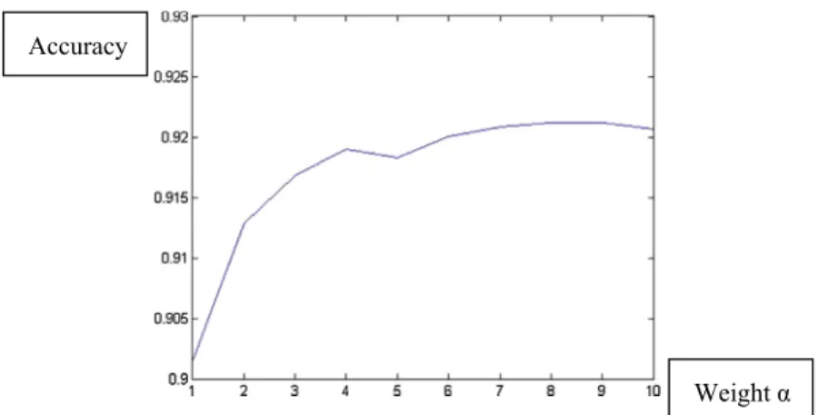
the SIFT and LBP descriptors coupled with SML classifier): the resulting performance of this ensemble is better than the single approaches (seeTable 5for each of these performances). According toTable 4, the fusion between (FM +[25]) and FV produces a performance improvement if the weighing fac-tor is accurately tuned. InFig. 2we show the performance of the ensemble based on SML (FM +[25]) and the best ensem-ble based on SVM (labeled FV) combined by weight sum rule as a function of the weighting factora. Before combining the two methods, the scores are normalized to mean 0 and stan-dard deviation 1. As can be observed, the fusion results in a slight performance gain (the result is up to 92.1% for
a= 8). More experiments need to be performed (e.g. using further training sets) to validate the usefulness of fusing SVM and SML.
Table 4 Accuracy obtained by our ensembles (in the first column, a short name used to refer the ensemble is reported).
Fusion short name Preprocessing Descriptors Matching FERET recognition rate LFW accuracy Fb Fc Dup1 Dup2
FM All POEM + MBC SML – – – – 90.0
FV All POEM + MBC SVM – – – – 86.6
FM +[25] – – – – – – – 91.7
FV +a(FM +[25]) – – – – – – – 92.1 All POEM Angle 98.7 100 93.1 92.7 – All MBC Angle 98.5 100 91.8 89.3 – FA All POEM + MBC Angle 99.2 100 94.6 94.0 –
Table 5 Comparison among the proposed ensemble with the state-of-the-arts approaches.
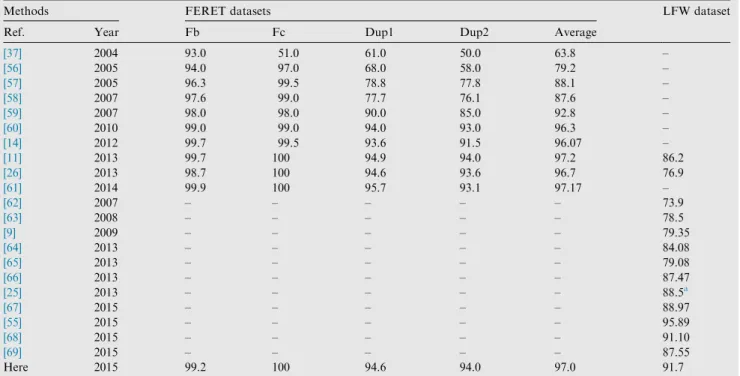
Methods FERET datasets LFW dataset
Ref. Year Fb Fc Dup1 Dup2 Average
[37] 2004 93.0 51.0 61.0 50.0 63.8 – [56] 2005 94.0 97.0 68.0 58.0 79.2 – [57] 2005 96.3 99.5 78.8 77.8 88.1 – [58] 2007 97.6 99.0 77.7 76.1 87.6 – [59] 2007 98.0 98.0 90.0 85.0 92.8 – [60] 2010 99.0 99.0 94.0 93.0 96.3 – [14] 2012 99.7 99.5 93.6 91.5 96.07 – [11] 2013 99.7 100 94.9 94.0 97.2 86.2 [26] 2013 98.7 100 94.6 93.6 96.7 76.9 [61] 2014 99.9 100 95.7 93.1 97.17 – [62] 2007 – – – – – 73.9 [63] 2008 – – – – – 78.5 [9] 2009 – – – – – 79.35 [64] 2013 – – – – – 84.08 [65] 2013 – – – – – 79.08 [66] 2013 – – – – – 87.47 [25] 2013 – – – – – 88.5a [67] 2015 – – – – – 88.97 [55] 2015 – – – – – 95.89 [68] 2015 – – – – – 91.10 [69] 2015 – – – – – 87.55 Here 2015 99.2 100 94.6 94.0 97.0 91.7
aObtained using the source code shared by the authors of[25]and the testing protocol described in this work (which is slightly different from
the one used in[25]).
3
Code available at http://empslocal.ex.ac.uk/people/staff/ yy267/software.html.
Finally, inTable 5a comparison with the state-of-art for both the FERET and LFW datasets is reported. Examining
Table 5, it is clear that system performance has significantly increased the last few years. In the LFW database, we report only those methods that use no outside training data (as in our proposed approach and as is the case with approaches classified in the Introduction as ‘‘shallow”). Notice that our proposed method is the second best approach on the LFW dataset after [55] (whose results are not reproducible, since the method is not available).
3.3. Deep features
As a final experiment, we test the proposed approach using a different set of features, the ‘‘learned”features that were con-trasted in the introduction with ‘‘handcrafted” features. Learned features are not defined in a straightforward manner to measure a specific property of the image (e.g. color and tex-ture) but are obtained from the internal representation of a CNN.
In this work, the well-trained CNN parameters reported in
[70]are used for representing the images in both the LFW and the FERET datasets. In particular, the CNN outputs of the
37th and 36th fully-connected layers are used for describing the images. These descriptors, whose dimensionality is 6718, are labeled LF in the following. CNN was trained once in
[70], and the same parameters are used in both our experiments on the LFW and the FERET datasets. Please note that in the present work CNN is used only for representation purposes and is trained on tiny cropped faces so that the background is minimally involved in classification. The matching step is performed by training a general-purpose classifier, viz., those reported inTable 6. For classifier training, the same protocols used in the previous experiments and detailed in Section3.1are employed (with no external images). Despite our attempts to line up settings for fair comparisons, it can be questioned whether the results reported inTable 6for the ‘‘learned fea-tures” (LF) can be fairly compared to the results we report above on the LFW database; this is because the LF descriptors have been obtained on a very large training set (even though external images were excluded from classifier training). Since the FERET protocol does not contain any limitations regard-ing the use of external images, the reported results are note-worthy: they are the highest published in the literature on the FERET datasets.
The results inTable 6demonstrate that the learned features have good discriminant power for this problem and confirm the learning capabilities of CNN. The results for learned features were obtained by aligning the face images so that eyes are cen-tered and by performing a tiny crop of the face (for the hand-crafted features). Moreover, no preprocessing step was per-formed since CNN was used solely for the purpose of feature extraction and was trained using nonprocessed images.
Before combining the two methods, the scores of the hand-crafted approaches (FM and FA) are normalized by dividing
Table 6 Accuracy obtained by the ‘‘learned-features”LF.
Fusion short name Descriptors Matching FERET recognition rate LFW accuracy Fb Fc Dup1 Dup2
Deep LF SML – – – – 93.22
FM + Deep – – – – – – 93.73
Deep LF Angle 99.92 99.48 92.11 91.88 – FA + Deep – – 99.75 100 98.48 99.15 –
Table 7 Computation time for the approach FM: Times are measured on an I5-3470 3.2 GHz – 8 GB Ram PC using nonoptimized MATLAB code.
FM T(PP) T(D) T(M) Total Single core 1.44 10.8 1.02 13.26 All the cores 0.42 2.92 1.02 4.36
Accuracy
Weight α
Figure 2 Weighted sum rule between FM and FV on the LFW dataset, and the weight of FV is fixed to 1, while the weight of FM varies between 1 and 10.S= FV +aFM.
their scores by the number of classifiers that built them. In both cases the fusion results in a performance gain, which reveals a partial independence among the features.
3.4. Computational analysis
In this subsection, we perform an analysis on the computa-tional cost of the general approach described in Section2. In this analysis, we refer to the method named FM.
The time complexityT(FM) of FM can be estimated as fol-lows:T(FM) =T(PP) +T(D) +T(M), whereT(PP),T(D),T
(M) denote the computational costs for the preprocessing steps, the extraction of descriptors, and matching, respectively.
T(D) includes the extraction of both descriptors (POEM and MBC) from all nine preprocessed images. The computation time of the feature transform, performed by PCA, is negligible. InTable 7computation times in seconds for the recognition of a single 9090 image on an I5-3470 3.2 GHz – 8 GB Ram PC using nonoptimized MATLAB code are reported.
The computation time for extracting the deep features (using a single core) is 0.55 s.
4. Conclusion
In this work, we proposed an ensemble of approaches that obtain good results on the LFW dataset and that produce the best performance on the FERET datasets (seeTable 6). Different preprocessing methods are coupled with two texture descriptors to improve performance. In the FERET datasets, where the aim is identification, we use the angle distance to match two faces. In the LFW dataset, where the aim is to ver-ify a given match, we use SVM and SML to match two faces. In the LFW dataset, the approach proposed here obtained 92.1% accuracy, which is the second best result reported in the literature without using outside training data. Unlike the sys-tem proposed in[55](which is the first), the code of our full system is freely available.
Furthermore, the proposed system fused with a method based on a set of ‘‘learned”features, results in the highest per-formance published in the literature on the FERET datasets, and it also works well on the LFW dataset.
In the future, we plan on testing new texture descriptors to enhance the performance of our approach. Future tests will also be performed using outside training data for comparisons of our approach with state-of-the-art deep learning methods trained with millions of examples. Preliminary results already reported in this work confirm that the ‘‘learned features”are a valid alternative to the ‘‘handcrafted features.”Moreover, since our last experiments were related to features learned for the face recognition task, in the future we are interested in evaluating the possibility of using features learned for differ-ent applications (i.e. object recognition, scene classification, etc.) in order to evaluate the degree of independence of such sets of features and their ability to work with different classifi-cation problems.
Author contributions
All authors made significant contributions.
References
[1]A. Cernea, J.L. Fernandez-Martı´nez, Unsupervised ensemble classification for biometric applications, Int. J. Pattern Recog. Artif. Intell. 28 (4) (2014) 1456007-1–1456007-32.
[2]L. Nanni et al, Effective and precise face detection based on color and depth data, Appl. Comput. Inf. 10 (1) (2014) 1–13. [3]S. Muruganantham, T. Jebarajan, A comprehensive review of
significant researches on face recognition based on various conditions, Int. J. Comp. Theory Eng. 4 (1) (2012) 7–15. [4]A.-A. Bhuiyan, C.H. Liu, On face recognition using gabor
filters, World Acad. Sci., Eng. Technol. 28 (2007) 51–56. [5]S. Chopra, R. Hadsell, Y. LeCun, Learning a similarity metric
discriminatively, with application to face verification, in: Conference on Computer Vision and Pattern Recognition (CVPR), 2005, pp. 539–546.
[6]M.A. Turk, A.P. Pentland, Eigenfaces for recognition, J. Cognit. Neurosci. 3 (1) (1991) 71–86.
[7]L. Wiskott et al, Face recognition by elastic bunch graph matching, IEEE Trans. Pattern Anal. Mach. Intell. 19 (7) (1997) 775–779.
[8]S. Lao et al, 3D template matching for pose invariant face recognition using 3D facial model built with isoluminance line based stereo vision, in: 15th IEEE International Conference on Pattern Recognition, IEEE, 2000, pp. 911–916.
[9]N. Pinto, J. DiCarlo, D. Cox, How far can you get with a modern face recognition test set using only simple features?, in: CVPR’09, 2009
[10] Z. Cao, et al., Face recognition with learning-based descriptor (2010) 2707–2714.
[11]N.-S. Vu, Exploring patterns of gradient orientations and magnitudes for face recognition, IEEE Trans. Inf. Foren. Secur. 8 (2) (2013) 295–304.
[12]N.-S. Vu, A. Caplier, Face recognition with patterns of oriented edge magnitudes, in: ECCV, 2010.
[13]Y. Liang et al, Exploring regularized feature selection for person specific face verification, in: ICCV, 2011.
[14]M. Yang et al, Monogenic binary coding: an efficient local feature extraction approach to face recognition, IEEE Trans. Inf. Foren. Secur. 7 (6) (2012) 1738–1751.
[15] Y. Taigman, L. Wolf, Leveraging Billions of Faces to Overcome Performance Barriers in Unconstrained Face Recognition, 2011 <http://arxiv.org/pdf/1108.1122.pdf>.
[16]N. Kumar et al, Attribute and simile classifiers for face verification, in: International Conference on Computer Vision (ICCV), 2009.
[17]T. Berg, P.N. Belhumeur, Tom-vs-pete classifiers and identity-preserving alignment for face verification, in: British Machine Vision Conference (BMVC), 2012.
[18]C. Chan et al, Multiscale local phase quantisation for robust component-based face recognition using kernel fusion of multiple descriptors, IEEE Trans. Pattern Anal. Mach. Intell. 35 (5) (2013) 1164–1177.
[19] Y. Taigman, et al., Deepface: closing the gap to human-level performance in face verification, in: Conference on Computer Vision and Pattern Recognition (CVPR), vol. 8, 2014. <http:// www.cs.tau.ac.il/~wolf/papers/deepface_11_01_2013.pdf>. [20]C. Lu, X. Tang, Surpassing human-level face verification
performance on LFW with GaussianFace, in: 29th AAAI Conference on Artificial Intelligence (AAAI), 2014, pp. 3811– 3819.
[21]Y. Sun, X. Wang, X. Tang, Deep learning face representation from predicting 10,000 classes, in: Conference on Computer Vision and Pattern Recognition (CVPR), 2014, pp. 1–9. [22]Y. Sun, X. Wang, X. Tang, Deep learning face representation
by joint identification-verification, in: NIPS, Montreal, 2014, pp. 1–9.
[23]Y. Sun, X. Wang, X. Tang, Deeply learned face representations are sparse, selective, and robust, in: Conference on Computer Vision and Pattern Recognition (CVPR), 2015.
[24]E. Zhou, Z. Cao, Q. Yin, Naive-Deep Face Recognition: Touching the Limit of LFW Benchmark or Not?, Cornell University Library, 2015
[25]Q. Cao, Y. Ying, P. Li, Similarity metric learning for face recognition, in: IEEE International Conference on Computer Vision (ICCV), 2013, pp. 2408–2415.
[26]L. Nanni et al, Ensemble of patterns of oriented edge magnitudes descriptors for face recognition, in: International Conference on Image Processing, Computer Vision, and Pattern Recognition (IPCV’13), 2013.
[27]T. Hassner et al, Effective face frontalization in unconstrained images, in: Computer Vision and Pattern Recognition (CVPR), 2015.
[28]Y.K. Park, S.L. Park, J.K. Kim, Retinex method based on adaptive smoothing for illumination invariant face recognition, Sig. Process. 88 (8) (2008) 929–1945.
[29]R. Gross, V. Brajovic, An image preprocessing algorithm for illumination invariant face recognition, in: 4th International Conference on Audio-and Video-Based Biometric Personal Authentication, 2003.
[30]V. Sˇtruc, N. Pavesˇic, Photometric normalization techniques for illumination invariance, in: V. Sˇtruc, N. Pavesˇic (Eds.), Advances in Face Image Analysis: Techniques and Technologies, IGI Global, Hershey, PA, 2011, pp. 279–300. [31]W. Chen, E. Meng-Joo, W. Shiqian, Illumination compensation
and normalization for robust face recognition using discrete cosine transform in logarithm domain, IEEE Trans. Syst., Man, Cybernet. Part B 36 (2006) 458–466.
[32]P.H. Lee, S.W. Wu, Y.P. Hung, Illumination compensation using oriented local histogram equalization and its application to face recognition, IEEE Trans. Image Process. (2012) 1–10. [33]D.J. Jobson, Z.u. Rahman, G.A. Woodell, A multiscale retinex
for bridging the gap between color images and the human observation of scenes, IEEE Trans. Image Process. 6 (7) (1997) 965–976.
[34] G. Heusch, F. Cardinaux, S. Marcel, Lighting normalization algorithms for face verification, IDIAP-com 05-03, 2005, p. 9. [35]X. Tan, B. Triggs, Enhanced local texture feature sets for face
recognition under difficult lighting conditions, Anal. Model. Faces Gestures (2007) 168–182, LNCS 4778.
[36]T. Zhang et al, Face recognition under varying illumination using gradientfaces, IEEE Trans. Image Process. 18 (11) (2009) 2599–2606.
[37]T. Ahonen, A. Hadid, M. Pietikainen, Face recognition with local binary patterns, in: ECCV’04, 2004, pp. 469–481. [38]N. Dalal, B. Triggs, Histograms of oriented gradients for human
detection, in: 9th European Conference on Computer Vision, San Diego, CA, 2005.
[39]M. San Biagio et al, Heterogeneous auto-similarities of characteristics (hasc): exploiting relational information for classification, in: ICCV13, 2013.
[40]G. Serra et al, Gold: Gaussians of local descriptors for image representation, Comput. Vis. Image Underst. 134 (May) (2015) 22–32.
[41]R.O. Duda, P.E. Hart, D.G. Stork, Pattern Classification, second ed., Wiley, New York, 2000.
[42]C.-C. Chang, C.-J. Lin, LIBSVM: a library for support vector machines, ACM Trans. Intell. Syst. Technol. (TIST) 2 (2011) 1– 39.
[43]N.-S. Vu, H.M. Dee, A. Caplier, Face recognition using the POEM descriptor, Pattern Recogn. Lett. 45 (7) (2012) 2478– 2488.
[44]P. Belhumeur, J. Hespanha, D. Kriegman, Eigenfaces vs. fisherfaces: recognition using class specific linear projection, IEEE Trans. Pattern Anal. Mach. Intell. 19 (7) (1997) 711–720.
[45]G. Csurka et al, Visual categorization with bags of keypoints, in: ECCV International Workshop on Statistical Learning in Computer Vision, 2004, pp. 59–74.
[46]R. Nosaka, C.H. Suryanto, K. Fukui, Rotation invariant co-occurrence among adjacent LBPs, in: ACCV Workshops, 2012, pp. 15–25.
[47]Z. Guo, L. Zhang, D. Zhang, A completed modeling of local binary pattern operator for texture classification, in: IEEE Trans. Image Process., 2010 (eoub.).
[48]J.L. Fernandez-Martı´nez, A. Cernea, Numerical analysis and comparison of spectral decomposition methods in biometric applications, Int. J. Pattern Recog. Artif. Intell. 28 (1) (2014) 14560–14593.
[49]J.L. Ferna´ndez-Martı´nez, A. Cernea, Exploring the uncertainty space of ensemble classifiers in face recognition, Int. J. Pattern Recog. Artif. Intell. 29 (3) (2015).
[50]J.L. Ferna´ndez-Martı´nez et al, Aligned pso for optimization of image processing methods applied to the face recognition problem, in: Swarm, Evolutionary, and Memetic Computing, Springer, Berlin, 2013, pp. 642–651.
[51]J.L. Fernandez-Martı´nez et al, From bayes to tarantola: new insights to understand uncertainty in inverse problems, J. Appl. Geophys. 98 (2013) 62–72.
[52]N. Cristianini, J. Shawe-Taylor, An Introduction to Support Vector Machines and Other Kernel-Based Learning Methods, Cambridge University Press, Cambridge, UK, 2000.
[53]J. Phillips et al, The feret evaluation methodology for face-recognition algorithms, IEEE Trans. Pattern Anal. Mach. Intell. 22 (2000) 1090–1104.
[54]G.B. Huang et al, Labeled Faces in the Wild: A Database for Studying Face Recognition in Unconstrained Environments, University of Massachusetts, Amherst, 2007.
[55]S.R. Arashloo, J. Kittler, Class-specific kernel fusion of multiple descriptors for face verification using multiscale binarised statistical image features, IEEE Trans. Inf. Foren. Secur. 9 (12) (2014) 2100–2109.
[56]W. Zhang et al, Local Gabor binary pattern histogram sequence (LGBPHS): a novel non-statistical model for face representation and recognition, in: IEEE International Conference on Computer Vision, ICCV’05, Beijing, 2005.
[57]W. Deng, J. Hu, J. Guo, Gabor-eigen-whiten-cosine: a robust scheme for face recognition, in: W. Zhao, S. Gong, X. Tang (Eds.), Second International Workshop, AMFG, Beijing, China, 2005, pp. 336–349.
[58]B. Zhang et al, Histogram of Gabor phase patterns (HGPP): a novel object representation approach for face recognition, IEEE Trans. Image Process. 16 (1) (2007) 57–68.
[59]X. Tan, B. Triggs, Fusing Gabor and LBP feature sets for kernel-based face recognition, in: Analysis and Modelling of Faces and Gestures, LNCS, vol. 4748, Springer, NY, 2007, pp. 235–249.
[60]S. Xie et al, Fusing local patterns of Gabor magnitude and phase for face recognition, IEEE Trans. Image Process. 19 (5) (2010) 1349–1361.
[61]Z. Chai et al, Gabor ordinal measures for face recognition, IEEE Trans. Inf. Foren. Secur. 9 (1) (2014) 14–26.
[62]E. Nowak, F. Jurie, Learning visual similarity measures for comparing never seen objects, in: Computer Vision and Pattern Recognition (CVPR), 2007.
[63]L. Wolf, T. Hassner, Y. Taigman, Descriptor based methods in the wild, Science 6 (2008) 1–14.
[64]H. Li et al, Probabilistic elastic matching for pose variant face verification, in: Computer Vision and Pattern Recognition, 2013, pp. 3499–3506.
[65]S.R. Arashloo, J. Kittler, Efficient processing of mrfs for unconstrained-pose face recognition, in: IEEE Sixth International Conference on Biometrics: Theory, Applications and Systems (BTAS), 2013, pp. 1–8.
[66]K. Simonyan et al, Fisher vector faces in the wild, in: British Machine Vision Conference, 2013, pp. 8.1–8.11.
[67]H. Li, G. Hua, Hierarchical-pep model for real-world face recognition, in: IEEE Conference on Computer Vision and Pattern Recognition (CVPR), 2015, pp. 4055–4064.
[68]H. Li et al, Eigen-pep for video face recognition, in: Computer Vision (ACCV 2014), 2015, pp. 7–33.
[69]F. Juefei-Xu, K. Luu, M. Savvides, Spartans: single-sample periocular-based alignment-robust recognition technique applied to non-frontal scenarios, Image Process. 24 (23) (2015). [70]O.M. Parkhi, A. Vedaldi, A. Zisserman, Deep face recognition,