Multistage Logistic Network Optimization under Disruption Risk

Multistage Logistic Network

Optimization under Disruption Risk

January, 2013

DOCTOR OF ENGINEERING

Muhammad Rusman

ABSTRACT

Getting over disruptions risk has been a challenging issue for many companies under the globalization that will link to potential external source such as demand uncertainties, natural disasters, and terrorist attacks. The disruption is an unexpected event that disturbs normal flows of products and materials within a supply chain. The disruption at one members of supply chain will propagate the offers and finally affect significant impacts on the entire chain. If we look back at the natural disasters in the recent decade, we know the supply chain activities have been put at the edge of high risk that bring catastrophic impact to companies. Not only such disruptions in the supply chain are increasing in frequency, but also the severity of their impact is escalating in terms of costs and losses. Since they will eventually bring a company a partial or complete halt, it is avoidable to consider disruption as a potential threat to supply chain and logistic network. Thereat, we can anticipate the disruption by considering preventive action to ensure the supply chain. If the supply chain takes preventive action against the disruption, such action is viewed as mitigation planning.

In this research, we analyzed possible strategies that a company can apply to mitigate and minimize the impacts of supply chain disruptions and design supply chain network in which facilities are unreliable by considering the fact that the facility members may fail. Failure of the facility means that the facility is no longer available to serve its customers. When these facilities

happen to fail, the concerned organization has to find alternate sources of supply to continue service to the customers, to reroute assignments that were initially intended or to incur large penalties.

To cope with the problem, we are interested in a three echelon logistic networks composed of distribution center (DC), relay station (RS) and Customer. Thereat, we consider two kinds of relay station like reliable relay station (RRS) and unreliable relay station (URS). The URS is subject to failures and the reliable relay station (RRS) becomes the hardened ones by having additional capacity or external alternative sourcing strategy. So it is more expensive to establish or operate such facility compared to URS. If the primary facility is disrupted, however, RRS will act as backup facilities to provide supply of product to customers.

Under those conditions, we formulate the logistic optimization problem so that the expected total cost associated with disruption probability is minimized under various constraints. It refers to a probabilistic mixed-integer programming problem. Then, this dissertation concerned three main problems. The first problem considers three types of allocation model, i.e., multi-multi allocation, multi-multi-single allocation and single-single allocation model. Taking these models, we compared some properties among three allocation models which have different configurations of the network. This is because the configuration is one of the most important and strategic issues in the logistic network design that has long lasted effect. Concern with this issue, we carried out a morphological analysis in order to measure the complexity of the multi stage logistic networks besides the expected cost. Finally, numerical experiment is carried out by applying commercial software to validate the proposed idea.

The operational level of the company will decrease below the normal condition when disruption occurs. The backup source after the disruption should be recovered not only as soon as possible, but also as much as possible.

(BCM/P) to reduce the recovery time objective. The second problem considers a robust supply chain network design by considering the effect of continuity rate to cope with the more practical circumstances. That is to say, we assume that URS is not completely halted and RRS will decrease the backup ability depending on the continuity rate of facility. Eventually, the continuity rate is percentage of ability facility to provide backup allocation to customers in abnormal situation and will affect the investment and operational costs. We evaluated the effect of the continuity rate for the foregoing three models. Finally, numerical experiment is carried out to derive some prospects for the future studies.

In the real-world situation, we need to concern huge numbers of facility members that make the resulting problem extremely difficult to solve. Accordingly, with increasing problems size, it becomes almost impossible to solve the problem by any currently available software. In the last problem, therefore, we developed an effective hybrid method so that we can solve the problem regardless of the size. The approach is composed of meta-heuristic method like tabu search and graph algorithm. Some bench mark problems are solved to validate the effectiveness.

Thesis Committee

Professor Yoshiaki Shimizu

Department of Mechanical Engineering Industrial Systems Engineering

Toyohashi University of Technology

Professor Zhong Zhang

Department of Mechanical Engineering Instrumentation Systems Laboratory Toyohashi University of Technology

Associate Professor Naoki Uchiyama

Department of Mechanical Engineering Robotics and Mechatronics Laboratory Toyohashi University of Technology

Associate Professor Rafael Batres

Department of Mechanical Engineering Industrial Systems Engineering

ACKNOWLEDGEMENTS

It has been an exceptional journey – one I had always dream of. I thank God, first and foremost, who ordained this entire journey and let me through it. For providing support, courage, and faith throughout it, I praise His name.

First I would like to express my deepest and sincere gratitude to Prof. Yoshiaki Shimizu for his guidance, expertise, time and patience throughout the course of my studies. His supports helped me tremendously in every stage of the research work. He patiently corrected and read my work in detail. This dissertation is immeasurably better as a result of his valuable comments, and he is a true model role to me.

I am deeply grateful to Associate Professor Dr. Rafael Batres who always support and enrich my perspective on research more than I could imagine. His knowledge and inspiration will remain me always. I would deeply thank to Dr. Tatsuhiko Sakaguchi for his supporting during this study. Additionally, profound thanks is due to the secretary of industrial systems engineering laboratory, Ms. Nakao Yoshiko, for her kindness and helpful throughout this study. I also want to thank my fellow students at Industrial Systems Engineering Laboratory for sharing their knowledge, wisdom, and inspiration.

Finally, I can only hope to describe my deepest love and sincere gratitude to my lovely mother who always there for me when I need her, and to my wife, who sacrificed her time, energy, and career because of her love for me and our dreams as a family and to my daughters, who provided the source of my motivation on a daily basis.

CONTENTS

Chapter 2 Literature Review ... 7

2.1 Supply Chain Management ... 7

2.2 Supply Chain Risk Management ... 9

2.3 Supply Chain Disruptions ... 12

2.4 Risk Drivers of Supply Chain ... 16

2.5 Supply Chain Risk Mitigation ... 17

2.5.1 Contingency Planning ... 19

2.5.2 Robust Optimization ... 20

2.5.3 Stochastic Models ... 22   

Chapter 3 Comparison of Multistage Logistic Network Designs ... 23

3.1 Introduction ... 23

3.2 Problem Formulation ... 26

3.2.1 Multi-multi allocation model (MMA Model) ... 29

3.2.2 Multi-single allocation model (MSA Model) ... 32

3.2.3 Single-single allocation model (SSA Model) ... 34

3.3 Numerical experiments ... 36

3.3.1 In case of MMA Model ... 37

3.3.2 In case of MSA Model ... 39

3.3.3 In case of SSA Model ... 41

3.4 Comparison of Results ... 42

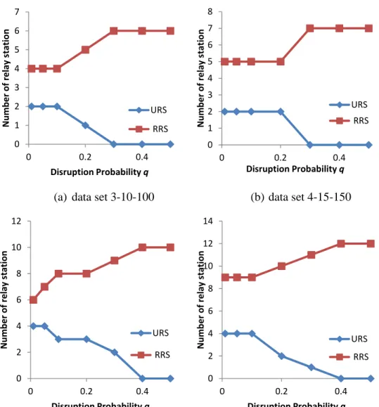
3.5 Larger Data Experiments ... 44 

3.6 Sensitivity Analysis ... 50 

3.7 Conclusion ... 54

Chapter 4 Morphological Analysis ... 55

4.1 Introduction ... 55

4.2 Business continuity management/plan ... 58

4.3 Morphological analysis ... 61

4.4 Conclusion ... 64

Chapter 5 Effect of continuity rate ... 65

5.1 Introduction ... 65

5.2 Problem Formulation ... 68

5.2.1 Without and with model comparison ... 69

5.2.2 Continuity Rate ... 72

5.2.3 Multi-multi allocation model (MMA model) ... 76

5.2.3 Multi-single allocation model (MSA model) ... 77

5.3 Numerical Experiment and Discussion ... 79

5.3.1 Results for small size model ... 80 

5.3.1 Results for large size model ... 86

5.4 Conclusion ... 90 

Chapter 6 Hybrid Approach for Huge MMA network... 91

6.1 Introduction ... 91

6.2 Problem formulation ... 92

6.3 Hybrid approach for solution ... 95

6.4 Numerical experiments and discussions ... 98

6.5 Conclusion ... 103 

Chapter 7 Conclusion and Future works ... 105

7.1 Conclusion ... 105 7.2 Future works ... 107   References ... 109 List of Publications ... 117   

List of Figures

Figure

2.1 An illustration of the company’s supply chain ... 8

2.2 Source of risk within supply chain ... 11

2.3 Illustration of Flexibility or agility, robustness and resilience ... 12

3.1 The structure of traditional multistage logistic network ... 24

3.2 Allocation model (a) MMA (b) MSA (c) SSA ... 25

3.3 Illustration of logistic network model under disruption risk ... 26

3.4 MMA model with disruption probability 0.01 ... 38

3.5 MMA model with disruption probability 0.5 ... 38

3.6 MSA model with disruption probability 0.01 ... 40

3.7 MSA model with disruption probability 0.5 ... 40

3.8 SSA model with disruption probability 0.01 ... 41

3.9 The Expected cost under various model (MMA and MSA) and disruption probabilities for data size (3-10-100) and (4-15-150) ... 45

3.10 The Expected cost under various model (MMA and MSA) and disruption probabilities for data size (5-20-200) and (6-25-250) ... 46

3.11 Number of open relay station for each disruption probabilities q ... 49

3.12 Sensitivity analysis of q and r – MMA model with data set (5-20-200) ... 50

3.13 Sensitivity analysis of q and r’ ... 51

4.1 An essence of BCP concept ... 60

4.2 Relation between total cost and simplicity ... 64

5.1 The difference configuration for w/o and w model ... 70

5.2 Comparison of continuity rates ... 72

5.3 Scheme of fixed charge against continuity rate ... 73

5.4 Continuity rate graph for shipping and handling cost ... 74

5.5 Relative difference against disruption ... 82

5.6: MMA model comparison between w (a) and w/o (b) model for Low-High continuity rate setting ... 83

5.7 Relative difference against disruption probability for each allocation model ... 84

5.8 Relative difference against disruption for large size problem. ... 89

6.1 Transformed graph from Physical flow ... 95

6.2 Flowchart of the proposed procedure ... 98

6.3 Profile of cost against disruption probability ... 99

6.4 Figure 6.4: Number of RS and its breakdown (#1~8: q=0.01, 0.03, 0.05, 0.1, 0.2, 0.3, 0.4, 0.5) ... 99

6.5 Profile of costs against disruption probability (level 1-3: q=0.01, 0.1, 0.5; Expected: solid; Primal: shade; Backup: open) ... 100

6.6 Number of RS and its breakdown (level 1-3: q=0.01, 0.1, 0,5) ... 101

6.7 Profiles of convergence ... 102

List of Tables

Table

2.1 Categories of supply chain disruptions ... 15

2.2 Classification of risk driver ... 18

3.1 Number of decision variable and constraints ... 37

3.2 Summary of the case solution for MMA, MSA and SSA model ... 43

3.3 Summary of the case solution for MMA, MSA with data set 5-20-200 .... 48

5.1 Parameter values for small size model ... 79

5.2 Parameter values ... 80

5.3 Continuity rate of the facility (rU, rR) ... 81

5.4 Comparison result among three models for (2-5-50) problem ... 85

5.5 Result of MMA for 4-15-150 ... 87

5.6 Result of MSA for 4-15-150 ... 87

5.7 Result of SSA for 4-15-150 ... 87

5.8 Result of MMA for 6-25-250 ... 88

5.9 Result of MSA for 6-25-250 ... 88

5.10 Result of SSA for 6-25-250 ... 88

Chapter 1

INTRODUCTION

1.1

Background

Supply chain disruptions have been a challenging issue for companies under the globalization environment. They are unplanned and unanticipated events that disrupt the normal flow of products and materials within a supply chain. The disruption at one members of supply chain can result significant impact on the entire chain. Supply chains are subject to potential external sources of disruption such as natural disasters and terrorist attacks. Research has been conducted by Kleindorfer and Saad (2005) and Wagner and Bode (2007) to illustrate the high priority supply chain disruptions should be in supply chain management. However, there is still a lot of work to be done in measuring the effects of disruptions on supply chain performance.

If we look back at the natural disasters in the last few years such as the latest earthquake and tsunami in Japan in March 2011, devastating floods in Thailand, and an extreme winter in Europe in early 2012, companies have been put at the edge of high risk due to frequent natural events that bring catastrophic impact to companies. Issues mentioned above can bring devastating impacts on the company’s operations and particular on its supply chain and logistics.

Chapter 1  

As an example when earthquake and tsunami in Japan caused dramatic impact on the supply chains and logistic distribution of many companies, including those in the automotive, electronics and chemical industries. The resulting slowdowns and cessation of operations affected seriously some companies. For example, a Hitachi factory that produces electronic components for European car maker was disrupted by this disaster. As a consequence, a certain European maker was argued to slow the production due to shortage of material from Hitachi.

We can anticipate the disruption by considering preventive action to ensure the supply chain is not adversely affected. If the supply chain takes preventive action against the disruption, such action is viewed as mitigation planning. Under such mitigation plan, the supply chain can build a robust system that will minimize the impact of the disruption in the future. One such mitigation mechanism would be to have backup facilities that may provide supplies if the primary facility would be disrupted. Schmitt (2011) recommended that one of the best protections can be achieved through backup capabilities that will protect the supply chain until the disruption’s end and prevent long or permanent interruptions to customer.

In line with a growing trend of natural disasters the complex and long supply chain due to increasing pressure to source globally and to exploit lower manufacturing costs made it even more difficult to avoid supply chain risks. The complexity of products and processes are also adding to the probability of disruptions.

Although an organization cannot prevent the occurrence of natural disasters, it can prevent or reduce the risk of damage from them. There are many tools and measures that an organization can apply in advance such as supply chain risk mapping and risk assessment to identify its characteristics of the supply chain flows (Xanthopoulos et al. 2012). Global companies tend to have more experience in dealing with disruption with more alternative

Chapter 1

necessary for companies to redesign a resilient supply chain strategically that resists the effect of a disruption.

1.2

Objectives of thesis

The objectives of this thesis are concerned with developing a robustly designed supply chain network that takes into account contingency plans in the event of disruption and providing a framework that consists of the strategies and analytics in designing supply chain networks to hedge against disruptions.

In this research, we analyzed possible strategies that a company can apply to mitigate and minimize the impacts of supply chain disruptions and design supply chain network in which some facilities are unreliable by considering the fact that facilities (such as manufacturing plants and warehouses) can fail. Failure of the facility means that the facility is no longer available to serve its customers. When these facilities fail, the concerned organization has to find alternate sources of supply to provide service to the customers and/or reroute assignments that were initially intended to go to a particular warehouses or retail location or incur large penalties. When a supply chain is poorly configured, finding alternate supply sources and rerouting shipments can be very expensive. In this study, we focus on issues related to facility disruptions. This is because facility disruptions are likely to be more critical than other supply chain drivers such as transportation, procurement, production, inventory, distribution, and routing.

The occurrence of any disruption is thus stochastic, so preventive measures can be taken to anticipate the disruption to ensure that the supply chain is not adversely affected. If a supply chain takes preventive measures in anticipation of a disruption then such actions are referred to as mitigation planning. Under a mitigation plan, the supply chain tries to build a robust system that can minimize the ill-effects of the disruption which is expected to

Chapter 1  

happen at some point in the future. Having backup suppliers and manufacturers is a part of the mitigation mechanism that provides supplies in the event when the facility is disrupted. Such cases are considered in Tomlin (2006) where a supply is considered from two suppliers one of which is reliable, but expensive, while the other is unreliable but cheap.

Mitigation planning of such kind is very popular in industries where the possibility of disruption is high, and it may cause immense financial ruin to the supply chain if they do not have backup source of supplies. Such was the case as demonstrated in Tomlin (2006) where he discussed the difference between Ericsson’s and Nokia’s strategies after the supply line for some parts for the cellular phone market was disrupted at their supplier, Phillip’s facilities. Nokia was able to minimize its losses by having a robust supply chain in the place where it could get its supplies from secondary suppliers. Meanwhile, Ericsson suffered a huge loss during this period because it had not anticipated this disruption and could not get the necessary supplies from elsewhere. This is just one of the numerous examples that demonstrate the need for some mitigation planning in place for the supply chains to remain competitive and profitable in the marketplace.

In spite of all the preventive actions, if disruptions do occur, proper policy changes should be made among the various members of the supply chain so that the supply chain can be brought back to its normal level relatively quickly. This field of study that deals with policy changes that a supply chain should take after a disruption has taken place is called contingency planning. In this research, we introduce the concept of business continuity management/plan as a part of the contingency planning in the event of disruptions.

Chapter 1

The definition of business continuity management/plan is a holistic management process that identifies potential impacts that threaten an organization and provides a framework for building resilience and the capability for an effective response to ensure that the recovery process is achievable without significant disruption to an organization (Gibb and Buchanan 2006).

Since every problem in this study is formulated as a mixed integer programming, a hybrid tabu search approach as heuristics method is applied to account for large-size problems.

We summarize the objective of this research as follows:

1. Comparing allocation models for multistage logistic network considering disruption risk.

2. Introducing morphological analysis for multistage logistic network considering disruption risk.

3. Proposing continuity rate as a part of business continuity plan approach. 4. Proposing an effective hybrid method composed of the metaheuristic

method and graph algorithms to offset potential losses from network disruption.

1.3

Overview of the thesis

This thesis composed of seven chapters. The first chapter describes the introduction. It includes background, objectives of the thesis and overview of the thesis. Chapter two concerns with literature review. This review includes the supply chain management concept, supply chain risk management concept, supply chain disruption, risk driver of supply chain, and supply chain risk mitigation.

Chapter 1  

Chapter three concerns about comparison of multistage logistics network designs. Chapter four describes the morphological analysis. Chapter five focuses on effect of continuity rate. Chapter six concerns about hybrid approach for huge multi-multi allocation model. The conclusion and recommendation for further study is lastly presented in Chapter seven.

Chapter 2

Chapter 2

LITERATURE REVIEW

2.1

Supply Chain Management

Modern supply chains today are becoming longer and more complex due to increasing market globalization (Thomas and Griffin 1996). Longer and complex supply chains are much more vulnerable to disruptions risk, which influence throughout the network and make planning more difficult. Robust and flexible supply chain designs become a significant consideration to the decision maker.

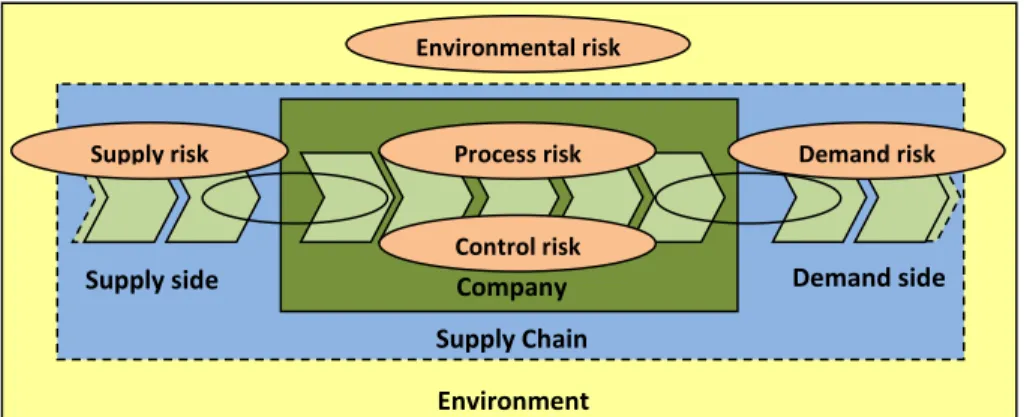
A supply chain is a system of facilities or a network of entities such as manufacturers, suppliers and distributors are working together to provide product to the end customers since raw material to finished product. Chen and Paulraj (2004) provide an illustration of a company supply chain which consists of a network of materials, information, and services processing links with the characteristics of supply, transformation and demand as shown in Figure 2.1.

In the 1990s, the concept supply chain management (SCM) was appeared to express the need to integrate the key business processes, from end user through original suppliers. Original suppliers are those that provide products, services and information that add value for customers and other stakeholders. Harland (1996) describes supply chain management (SCM) as

Chapter 2

managing business activities and relationships (1) internally within an organization; (2) with immediate suppliers, (3) with first and second-tier suppliers and customers along the supply chain, and (4) with the entire supply chain. The main purpose to apply the concept of SCM to the organization is to produced the product and distributed at the right quantities, to the right locations and at the right time, in order to minimize system wide costs (or maximize profits) while satisfying service level requirements.

Figure 2.1: An illustration of a company's supply chain

The basic idea behind the SCM is that companies and corporations involve themselves in a supply chain by exchanging information regarding market fluctuations and production capabilities. Supply chain decisions include: Which suppliers should we use? How many manufacturers and distributors should we have and where should we locate them? How do we determine the capacity at each location? What products should manufacturers produce? Given locations and capacities, supply chain decisions will then try to answer questions such as the following: what quantities should we produce and store at these locations? What quantities should be moved from location to location and at what time? (Shen 2007).

Chapter 2

One of the crucial planning activities in SCM is to design configuration of the supply chain network. In SCM, there are three planning levels, namely strategic, tactical and operational, which usually distinguished depending on the time horizon (Melo et al. 2009). The planning of the strategic level includes determining the number, location, capacity and technology of the facilities and the tactical/operational level involves determining the quantities of purchasing, production, distribution, product handling and inventory holding as well as transportation between established facilities. The configuration of the supply chain is the key strategic decision that influences activities at a tactical/operational level and has long-lasting effect on network (Shen 2007). Therefore, the fact that asupply chain network design (SCND) problem invests a large amount of capital for new facilities become an important issue.

Organizations as well as entire supply chain network become more vulnerable against disruption risks. Therefore, it is essential for organizations in supply chain to agree on a common risk management approach in their network design. One drawback of SCM is the assumption that process will run under normal conditions without considering potential risks that might occur. Risk can be arising from the supply side, demand side as well as from facility side become great a concern in today’s business environment. The concept of the supply chain risk management has been developed in the literature and practice to handle this risk.

2.2

Supply Chain Risk Management

Companies have to offer a wide range of different products or variants in order to satisfy customer demand which leads to higher vulnerability due to higher complexity (Harland et al. 2003). Furthermore, companies can no longer afford to focus on local markets. They are forced to realize the potential of global markets in terms of suppliers as well as customers resulting in a

Chapter 2

highly complex supply chain. Due to a high interconnectedness of companies and trend towards globalization within complex networks, supply chains have become more vulnerable for risk disruptions.  

Supply chain risk is recognized in today’s economy as a major threat to business continuity. A disruption in the supply chain can reduce a company’s revenue, decrease its market share, inflate costs, or threaten production and distribution. In recent years, many companies implement the concept of supply chain risk management (SCRM) to enhance the resilience against the disruption risk. According to Wieland and Wallenburg (2012), SCRM can be defined as the implementation of strategies to manage both everyday and exceptional risks along the supply chain based on continuous risk assessment with the objective of reducing vulnerability and ensuring continuity.

A common classification of supply chain risk was classified into five sources according to their origin. These five sources can be summarized in three groups: company internal risks, supply chain internal risks, and environmental risks as depicted in Figure 2.2 (Christopher and Peck 2004). Two risk sources, process and control risks, are located within the company considered. These sources cover all risks emerging out of production and logistics processes as well as managerial risks, which fulfill the definition of supply chain risks. The second group consists of two other risk sources, supply and demand risks. These sources contain all risks emitted by supply chain partners, thus all indirect supply chain risks. The last group is formed by the environmental risks. These risks represent all potential damage caused by socio-political, macroeconomic or natural disasters.

Chapter 2

Figure 2.2: Source of risk within supply chain

According to Chopra and Sodhi (2004), the supply chain risks could be in the form of delays of materials from suppliers, large forecast errors, system breakdowns, capacity issues, inventory problems, and disruptions. Another classification which is categorized supply chain risks into operations and disruptions risks (Tang, 2006). The operations risks are associated with uncertainties inherent in a supply chain, which include demand, supply, and cost uncertainties while disruption risks are those caused by major natural and man-made disasters such as flood, earthquake, tsunami, and major economic crisis. Tang (2006) reviewed SCRM articles, but the author focused on quantitative models. The author classified articles according to four basic supply chain areas: supply management, product management, information management, and demand management.

Risk and uncertainty has always been an important issue in supply chain management. Earlier literature consider risks in relation to supply lead time reliability, price uncertainty, and demand volatility which lead to the need for safety stock, inventory pooling strategy, order split to suppliers, and various contract and hedging strategies (Tang 2006). The author believes that effective SCRM has become a need for companies nowadays.

Environmental risk

Demand risk 

Supply risk  Process risk

Control risk Supply side  _Company 

Supply Chain 

Environment 

Chapter 2

Several words mostly mention on related to SCRM concept in various ways: robustness, flexibility and resilience. The difference between robustness, flexibility and resilience is illustrated in the figure 2.3 (Husdal 2009). The ability to survive (resilience) is likely to be more important in a business setting than the ability to regain stability (robustness) or the ability to change course (flexibility or agility) quickly. Supply chain risk management must include all.

Figure 2.3: Illustration of Flexibility or agility, robustness and resilience

2.3

Supply Chain Disruptions

Supply chain disruptions are unplanned events that can affect the normal, expected flow of materials, information, and products, and are recognized as inevitability within a supply chain organization (Svensson, 2002).

  Flexible/Agile Future Now Resilient Future Now Robust Future Now

Chapter 2

This is not a matter of a supply chain system encountering a problem, but rather a matter of when a problematic event will occur and the severity of the event. Therefore, the study of risk, interdependence, and the associated impact of a disruption on supply chain performance is a growing area of interest to many as they strive to reduce their organization’s risk of disruption.

There are some previous studies about supply chain risk considering disruption risk. For instances, the research of Tomlin (2006) investigates the impact of considering unreliable facilities for the facility location problems. Snyder and Daskin (2005) and Lim et al. (2009) have introduced facility location model, in which facility may fail with given probability while Chopra and Sodhi (2004) and Kleindorfer and Saad (2005) studied the risk management perspective on supply chain disruption.

Supply chain disruption can be the result of large-scale natural disaster, terrorist attacks, plant fires, electrical blackouts, financial or political crises, and many other scenarios. Supply chain disruptions are the enemy of all companies for, both potential and actual condition. Definition of disruption in term of the supply chain context is unplanned and unanticipated events that disrupt the normal flow of products and materials within a supply chain (Craighead et al. 2007). Some well-known examples of supply chain disruptions include:

• The 1999 earthquake in Taiwan had a dramatic impact on the global semiconductor market. At the time, Taiwan was the third largest supplier of computer peripherals in the word, so the earthquake caused a temporary global shortage of semiconductor components with the production down times that ranged from 2-4 weeks. Production and sales of many firms were profoundly affected by this shortage (Bundschuh et al. 2003).

• On March17, 2000, a small fire occurred at a Philips semiconductor plant in Albuquerque, the New Mexico. Even though, the plant was

Chapter 2

burned for only 10 minutes but production process was halted. Nearly half of the factory’s output was destined for two Europe’s biggest cell phone makers, Nokia and Ericsson. When Nokia and Ericsson received information about the fire at the following day, they were informed that there would be minimal disruption. In fact, the factory took several months to return to full production (Sheffi 2001).

• On March 11, 2011, Tohoku area in Japan was struck by a 9.0-magnitude earthquake and follow by the massive tsunami. General Motors had to halt the production of vehicles at several plants, due to parts shortages from Japanese suppliers. Also, Toyota had to suspend production of parts in the mother country that were intended to be shipped overseas. Finally, most Japanese automotive assembly plants remain closed (Azad 2012).

Consequences of supply chain disruptions might be financial losses, a negative corporate image or a bad reputation eventually accompanied by a loss in demand as well as damages in security and health (Juttner et al. 2003). The MIT Research Group on “Supply Chain Response to Global Terrorism” identifies six different levels of disruption in the context of supply chain management (Rice et al. 2003). See Table 2.1.

Over the last several decades, significant effort has been expended in making supply chains leaner and cheaper. However, recent studies point out that while this effort has successfully reduced operational costs, unfortunately, it has also increased the vulnerability of supply chains (Rice et al. 2003). While companies are often used to dealing with supply chain risks arising at the operational level, many suffer much heavily from supply chain disruptions. Although supply chain disruptions occur with low probability, the consequences are usually catastrophic. Kleindorfer and Saad (2005) showed that disruption risks are fundamentally different from the risks arising from

Chapter 2

production and are likely to persist for a long period of time. The importance of disruption risk is also highlighted by Hendricks and Singhal (2005) who show that supply chain disruptions expose a firm to negative financial impacts; recovering from such shocks is typically very slow.

Table 2.1: Categories of supply chain disruptions

Failure Mode Description

Disruption in Supply Delay or unavailability of materials from suppliers leading to a shortage of inputs that could paralyze the activity the activity of the company

Disruption in Transportation Delay or unavailability of the transportation infrastructure leading to the impossibility to move goods, either inbound and outbound

Disruption at Facilities Delay or unavailability of plants, warehouses and office buildings hampering the ability to continue operations

Freight breaches Violation of the integrity of cargoes and products, leading to the loss or adulteration of goods (can be due either to theft or tampering with criminal purpose, e.g. smuggling weapons inside containers) Disruptions in communications Delay or unavailability of the information

and communication infrastructures, either within or outside the company, leading to the inability to coordinate operations and execute transactions

Disruption in Demand Delay or disruption downstream can lead to the loss of demand temporarily or permanently, thus affecting all the companies upstream

Chapter 2

2.4

Risk Drivers of Supply Chain

It is essential for constructing a resilient logistic network to capture the properties of risk imbedded thereat. Such risks are classified into three categories listed below.

• Outside risk refers to abnormal climate, natural disaster, change/enactment of law/regulation, riot, terrorism and exhaustion of resources, etc.

• Inside risk is

o caused by inbound logistics such as: crash; problems associated with quality, safety, productivity, tardiness and delivery of raw materials and parts; strike, scandal; violation of laws and regulations, etc.

o caused by outbound logistics such as: unexpected change of demand; problems from order processing and solvency; frequent deviations of specification, etc.

• Risk caused within the company refers to

o those peculiar to operations incidents, malfunctioning of production, human errors, etc.

o those caused by management and decision making, safety level of inventory, schedule of delivery, location/allocation of sites/resources, etc.

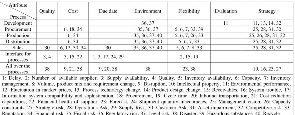
Cao and Chu (2010) provide classification of the risk driver in the supply chain in order to understand the conventional studies in a well-organized manner and to have a definite prospect in the future as shown in Table 2.2. In particular, they claim the importance of organizational cooperation over the society. Looking at the recent worldwide affairs, it makes sense prepare against various disruption risks and move on undertaking a suitable Business Continuity Plan/Management (BCP/BCM). This is also a

Chapter 2

consequence guided from the “All over the processes” row in the table. As a summary of this section, the importance of backup system for supply chain is well understandable for this purpose.

2.5

Supply Chain Risk Mitigation

Risk mitigation is to mitigate the uncertainties identified from the various disruption risk sources by undertaking some strategic move deliberately (Miller 1992). There are many strategies for mitigating disruption risks. Oke and Golapalakrishnana (2009) suggested some kinds of measure to mitigate supply risks, such as better planning and co-ordination of supply and demand, flexible capacity, identifying supply chain vulnerability points and having a contingency plan and multiple sourcing strategy. In the general classification of mitigation strategy for disruption risk are contingency plan, robust optimization and stochastic models.

Chapter 2  

Tabel 2.2: Classification of risk driver Attribute

Process

Quality Cost Due date Environment Flexibility Evaluation Strategy

Development 36, 37 11 11, 13, 14, 32 Procurement 6, 18, 34 35, 36, 37 5, 6, 7, 33, 39 25, 28, 31, 32 Production 6, 34 35, 36, 37, 40 5, 6, 7, 26, 33 25, 26, 28, 31, 32 Distribution 6, 34 35, 36, 37, 40 5, 6, 7, 33 25, 28, 31, 32 Sales 30 6, 12, 30, 34 30 35, 36, 37, 40 5, 6, 7, 8, 33 25, 28, 31, 32 Interface for processes 3, 4 3, 15, 22 1, 3, 17, 24, 29 2, 15, 19 All over the

processes 38 9, 21, 38 9, 20, 38 38 23, 38 10, 16, 23, 27 1: Delay, 2: Number of available supplier, 3: Supply availability, 4: Quality, 5: Inventory availability, 6: Capacity, 7: Inventory management, 8: Volume, product mix and requirement change, 9: Disruption, 10: Intellectual property, 11: Environmental performance, 12: Fluctuation in market prices, 13: Process technology change, 14: Product design change, 15: Receivables, 16: System trouble, 17: Information system compatibility and sophistication, 18: Procurement, 19: Cycle time, 20: Inbound transportation, 21: Cost reduction capabilities, 22: Financial health of supplier, 23: Forecast, 24: Shipment quantity inaccuracies, 25: Management vision, 26: Capacity constraints, 27: Strategic risk, 28: Operations Ask, 29: Supply Risk, 30: Customer Ask, 31: Asset impairment, 32: Competitive risk, 33: Reputation, 34: Financial risk, 35: Fiscal risk, 36: Regulatory risk, 37: Legal risk, 38: Disaster, 39: Hazardous substances, 40: Recycle

Chapter 2

2.5.1

Contingency Planning

Contingency planning is a risk management tool, and the aim is to minimize the impact of an upcoming event and show how the business will resume normal operations after the event of disruption. In business continuity and risk management, a contingency planning is a process that prepares an organization to respond the unplanned event. For simple definition, a contingency plan is can be referred to as "Plan B".

Contingency planning in supply chain has become a significant issue for manufacturers and distributors because supply chains are getting leaner, distances are growing longer and natural disasters such as earthquakes and hurricanes are always a threat. Lean supply chains eliminate inventory that in the past provided some buffer for unexpected events. Contingency planning in supply chain begins with identifying the potential risks. We have shown the categories of supply chain disruptions in Table 1 section 2.3.

In the context of the recovering from a supply chain disruption, both Ericsson and Nokia were facing supply shortage of critical cellular phone component (radio frequency chips) after Philip’s Electronics semiconductor plant in New Mexico caught on fire in March 2000. Philip’s informed Ericsson and Nokia that it was not possible to deliver certain components for a certain period after fire accident. Nokia recovers quickly by deploying a contingency plan to reconfigure the design of their generic cellular phone. So that, by this phone modification, Nokia can accept slightly a component that was different from the one being delivered by the Philips’s plant. The concept of product flexibility is applied by Nokia affecting recover easily from serious disruption. Nokia can provide difference product based on the generic cell phone without any significant problem. Consequently, Nokia satisfied customer demand and obtained a stronger market position. On the contrary, Ericsson was unable to deploy a similar strategy and it loss $400 million in sales (Hopkins 2005).

Chapter 2

2.5.2

Robust Optimization

Robust optimization is another approach to handle uncertainty in the planning stage. The philosophy of robust optimization is to help companies to reduce cost and/or improve customer satisfaction under normal circumstances and sustain their operations during and after disruption.

Tang (2006b) presented some robust strategies as listed below.

- Postponement; utilizes product or process design concept such as standardization, commonality, modular design and operational reversal. (Increase product flexibility).

For example, Nokia deployed a contingency plan by reconfigure its generic cell phone quickly to allow slightly different components. - Strategic Stock; instead of carrying more safety stocks, a company may

consider keeping some inventories at certain strategic locations to be shared by multiple supply chain partners (Increases product availability).

For example, CDC keeps large quantities of medicine and medical supplies at certain strategic locations in USA.

- Flexible Supply Base; To use more than two production bases, one for volume and the other for the excess in order to mitigate the risk associated with single sourcing (increases supply flexibility).

For example, HP used Singapore plant as the base volume and Washington one to produce the excess of the base volume.

- Make-and-Buy; Supply chain more resilient if certain products are manufactured in-house while others are outsourced to other suppliers (increases supply flexibility).

For example, Zara produce their fashion item at their in-house factories and outsource other basic items to their suppliers in China.

Chapter 2

- Economic Supply Incentives; Used at the condition that there are very limited numbers of suppliers available in the market (increases product availability).

For example, Supplier offered economic incentives by US government to re-enter the flu vaccine market by sharing some financial risks and committing to a certain quantity in advance at a certain price and buying the unsold products again at a lower price when the flu season end.

- Flexible Transportation; Transportation is the Achilles’ heel and consider adding more flexibilities in a proactive manner (increase flexibility in transportation).

For example, Multi-modal transportation (trucks, motorcycles, bicycles, ships and helicopters), multi-carrier transportation and multiple routes. - Revenue Management via dynamic pricing; Dynamic pricing is a

common mechanism for selling perishable products/services (increases control of product demand).

For example, Dell offered special low-cost-upgrade options to customers if similar computers with components from other supplier were chosen after an earthquake happened in 1999 and disrupted its Taiwan supplier.

- Assortment Planning; Reconfiguring the set of products on display, location on the shelves and number of facings for each product to manipulate customer’s product choice and demand (increases control of product demand).

For example, five supermarkets in USA suggest that one can utilize this strategy to entice customers to purchase widely available products when certain ones are facing SC disruptions.

- Silent Product Rollover; under this strategy, new products are leaked slowly into the market without any formal announcement (increase control of product exposure to customers)

Chapter 2

For example, Swatch produces each watch model only once and launches new products so that its customers will view all available ones as collectibles by utilizing this approach.

The advantages of robust strategies are that they can guarantee the performance of the supply chain regardless of the occurrence of major disruptions. Prevention is better than cure, if the company can reduce their exposure to risk by considering supply chain alliance network, lead time reduction and recovery planning system.

2.5.3

Stochastic Models

Stochastic model is a typical method of generating and operational plan within an uncertain environment when the precise probability distribution of future uncertainty is known in advance.

The common type of stochastic disruption appearing in the literature is supply disruption. Schmitt (2008) developed a stochastic model considering supply disruption include the impact to industry and demonstrate mitigation strategy in supply chain. Goh et al. (2007) develop a multistage stochastic model for supply chain network by providing a general formulation of the multi-stage supply chain network problem operating under a scenario of a variety of risks. The goal is to optimize distribution logistics and facility location planning in an international setting.

Chapter 3

COMPARISON OF MULTISTAGE

LOGISTIC NETWORK DESIGNS

3.1

Introduction

As the development of economic globalization, worldwide logistics become imperative for the business world especially by global company that services supported by universal supply chain. How to manage logistics system efficiently has become an important issue for many companies to reduce their total costs. In general, total cost is defined as the sum of production, supply, inventory, transportation, and facility costs.

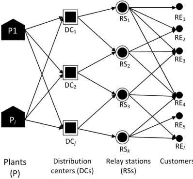
The traditional multistage logistics networks problem is defined as a set of facilities including potential suppliers, potential plant facilities, and distribution centers (DCs) and a set of customers with deterministic demands. The main purpose of this problem is to determine the configuration of the production and distribution system between facilities in order to satisfy the customer demands and the profit of the company is maximized or the total cost is minimized (Goetschalckx et al. 2002). The network structure of the traditional logistic problem is like that shown in Figure 3.1.

In this study, we focus on the issue related to facility disruption risk for multistage logistic networks and present three different kinds of allocation model each of which will provide a robust design. The proposed allocation

Chapter 3  

models are multi-multi allocation (MMA) model, multi-single allocation model (MSA) and single-single allocation (SSA) model. The aim of this study is to compare the properties among these allocation models. In the MMA model, each Relay Station (RS) will receive the product from multiple DCs and customers also from multiple RSs depending on the respective demand of the customer. In the MSA model, RSs will receive the product from multiple DCs while customers only from one RS. In the SSA model, each RS can receive just from a single DC, and each customer also receives from a single RS. Figure 3.2 shows the difference between the models.

Figure 3.1: The structure of traditional multistage logistic network  

Plants

(P)

P1

P

Chapter 3  

Previous research takes only account of two echelon logistic problems as explained in Chapter 2 section 2.3. In a real word application, logistic network design can be proposed as multistage problem. Therefore, we define the problem as a multistage logistic network designs problem.

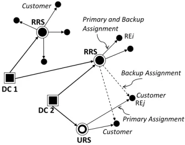
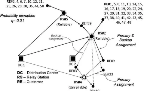
A three echelon problem consists of a set of distribution centers (DCs), a set of relay stations (RSs) and a set of customers (REs). The location decisions are made in the RS level. In RS level, we proposed two kinds of RS the reliable RS (RRS) and unreliable RS (URS). An unreliable relay station (URS) is subject to failures. Failure of the RS means that RS is no longer available to serve customers. When RS fails, the firm has to find alternate sources of supply to provide service to customers. A reliable relay station (RRS) has additional capacity and or an external alternative sourcing strategy. By default, it is more expensive to establish or operate RRSs compare to URSs. Figure 3.3 illustrates the multistage logistic network where RS is potentially being disrupted. Two DCs distribute products to three relay stations (RSs), which consist of two RRS and one URS. If the demand of the customer is satisfied by RRSs, then only one assignment is available for both primary and backup assignments. On the other hand, if the customer is assigned to URSs, backup assignment is required besides the primary assignment. This

Figure 3.2: Allocation model; (a) MMA (b) MSA (c) SSA   DC   RS   RE   Multiple allocation  Multiple allocation  Single allocation  Single allocation  Single allocation  Multiple allocation  (a)  (b)  (c) 

Chapter 3  

means when the disruption occurs at URS, the demand of customer will be distributed from RRS which is assigned as the backup.

Figure 3.3: Illustration of logistic network model under disruption risk

3.2

Problem Formulation

In this section, we present a Mixed-Integer Programming formulation for each of the proposed allocation models. The objective is to minimize total cost by properly locating reliable and unreliable facilities. The expected total costs that consists of fixed costs for opening RSs, shipping costs at DCs, transportation costs between each DCs to RSs and RSs to customers and handling cost at each RS. In these models, each customer k K _{has a demand} dk. The product is distributed from DC I to RS J and from RS J to customers K, respectively. At each customer k, we may locate either RRS with opening cost

FjR or URS with opening cost FjU. Fixed cost for opening RRS is higher than URS (FjR > FjU) due to an undisrupted reason.

The transportation cost per unit demand from DC I to RS J is given by

T1 P and T1 B for primary assignment and backup assignment, respectively.  

DC 1 

Backup Assignment 

Primary Assignment 

Primary and Backup 

Assignment  DC 2  RRS  URS  RRS  Customer  Customer  Customer  REj  REi 

Chapter 3  

We also consider the relation T1ijP < T1ijB due the consequence of using the backup resources. Similarly, the transportation cost per unit demand from RS to the customer is given by T2jkP and T2jkB for primary assignment and backup assignment, respectively. We also assume the relation T2jkP < T2jkB due to the consequence of using the backup resources.

Moreover, the handling cost at each RS is denoted as HkP and HkB for primary and backup condition, respectively. We assume that the relation HkP <

HkB. In this model, we assume the probability of disruption which is denoted by

qj (0<qj<1). Primary assignments occur with probability 1-qj under the normal cost while backup assignments occur with probability qj under the abnormal cost.

The following notations are used to describe the mathematical model.

Index set

I : set of distribution centers (DC)

J : set of relay stations (RS)

K : set of customers(RE)

Parameters

: Fixed cost for opening URS j

: Fixed cost for opening RRS j

: Shipping cost at DC as primary assignment : Shipping cost at DC as backup assignment

: Handling cost at RS as primary assignment : Handling cost at RS as backup assignment

Chapter 3  

1 : Transport cost from DC to RS as backup assignment 2 : Transport cost from RS to customer as primary assignment 2 : Transport cost from RRS to customer as backup assignment

: Capacity of RS

: Maximum supply ability of DC : Minimum supply ability of DC : Demand of customer

: Probability of disruption RS j 0 1

Decision variable

: Shipped amount from DC to RS as primary assignment : Shipped amount from DC to RS as backup assignment : Shipped amount from RS to customer as primary assignment

: Shipped amount from RS to customer as backup assignment

1, ; 0, . 1, ; 0, . 1, ; 0, . 1, ; 0, . 1, ; 0, . 1, ; 0, .

Chapter 3  

3.2.1

Multi-multi allocation model (MMA Model)

In this model, we consider each RS will receive the product from multiple DCs and customer also from multiple RSs depending on the respective demand of the customer. The model for MMA is described as follows. Minimize U U R R j j j j j J j J

F x

F x

+

∑

∑

(1

)

(

1 )

(

2 )

q

C

T

a

H

T

b

⎛

⎞

+

−

⎜

⎜

+

+

+

⎟

⎟

⎝

⎠

∑

∑

∑

(

1 )

(

2 )

q

C

T

a

H

T

b

⎛

⎞

+

⎜

⎜

+

+

+

⎟

⎟

⎝

⎠

∑ ∑

∑

J

j

x

x

+

≤

1

∀

∈

∑

≥

x

1

J

j

x

x

U

a

≤

+

∀

∈

∑

)

(

∑

∈

∀

≤

U

x

j

J

a

Chapter 3  

I

i

PU

a

≤

∀

∈

∑

I

i

PU

a

≤

∀

∈

∑

I

i

PL

a

≥

∀

∈

∑

I

i

PL

a

≥

∀

∈

∑

J

j

b

a

−

∑

=

∀

∈

∑

0

J

j

b

a

−

∑

=

∀

∈

∑

0

K

k

d

b

=

∀

∈

∑

K

k

d

b

=

∀

∈

∑

{ }

j

J

x

∈

0

,

1

∀

∈

{ }

j

J

x

∈

0

,

1

∀

∈

J

j

I

i

a

≥

0

∀

∈

,

∀

∈

J

j

I

i

a

≥

0

∀

∈

,

∀

∈

J

j

I

i

b

≥

0

∀

∈

,

∀

∈

J

j

I

i

b

≥

0

∀

∈

,

∀

∈

Chapter 3  

Equation (3.2) states that either of RRS or URS can be open, but not both. Equation (3.3) states that the model required locating at least one RRS. Equations (3.4) and (3.5) are capacity constraint for RS as primary and backup assignment, respectively. Equations (3.6) and (3.7) are upper bounds for available supply as primary and backup assignment, respectively. Equations (3.8) and (3.9) are lower bounds for available supply as primary and backup assignment, respectively. Equations (3.10) and (3.11) are balances of product flow as primary and backup assignment, respectively. Equations (3.12) and (3.13) mean demand of every customer must be satisfied as primary and backup assignment, respectively, Equations (3.14) and (3.15) are integrality restrictions on decision variables. Equations (3.16) - (3.19) are nonnegative constraints for primary and backup assignment amounts.

Chapter 3  

3.2.2

Multi-single allocation model (MSA Model)

In this model, we consider each RS will receive the product from multiple DCs while customer only from one RS. The model for MSA is described as follows: Minimize U U R R j j j j j J j J

F x

F x

+

∑

∑

(1

)

(

1 )

(

2 )

q

C

T

a

H

T

d y

⎛

⎞

+

−

⎜

⎜

+

+

+

⎟

⎟

⎝

⎠

∑

∑

∑

(

1 )

(

2 )

q

C

T

a

H

T

d y

⎛

⎞

+

⎜

⎜

+

+

+

⎟

⎟

⎝

⎠

∑ ∑

∑

K

k

y

=

∀

∈

∑

1

K

k

y

=

∀

∈

∑

1

K

k

J

j

x

x

y

≤

+

∀

∈

,

∀

∈

Chapter 3  

K

k

J

j

x

y

≤

∀

∈

,

∀

∈

J

j

y

d

a

−

∑

=

∀

∈

∑

0

J

j

y

d

a

−

∑

=

∀

∈

∑

0

{ }

j

J

k

K

y

∈

0

,

1

∀

∈

,

∀

∈

{ }

j

J

k

K

y

∈

0

,

1

∀

∈

,

∀

∈

In MSA model the explanation of the objective function and constraints are all equal to the MMA model except for equations (3.21) and (3.22). These equations express that each customer must be assigned to single RS both for the primary and backup assignment, respectively.

Chapter 3  

3.2.3

Single-single allocation model (SSA Model)

In this model, we consider each RS can receive just from single DC and customer also receives from single RS. The model for SSA is described as follows: U U R R j j j j j J j J

F x

F x

+

∑

∑

(1

)

(

1 )

(

2 )

q

C

T

a z

H

T

d y

⎛

⎞

+

−

⎜

⎜

+

+

+

⎟

⎟

⎝

⎠

∑

∑

∑

(

1 )

(

2 )

q

C

T

a z

H

T

d y

⎛

⎞

+

⎜

⎜

+

+

+

⎟

⎟

⎝

⎠

∑ ∑

∑

J

j

z

=

∀

∈

∑

1

J

j

z

=

∀

∈

∑

1

J

j

x

x

U

z

a

≤

+

∀

∈

∑

)

(

J

j

x

U

z

a

≤

∀

∈

∑

Chapter 3  

∑

∈

∀

≤

z

PU

i

I

a

∑

∈

∀

≤

z

PU

i

I

a

I

i

PL

z

a

≥

∀

∈

∑

I

i

PL

z

a

≥

∀

∈

∑

J

j

y

d

z

a

−

∑

=

∀

∈

∑

0

J

j

y

d

z

a

−

∑

=

∀

∈

∑

0

{ }

i

I

j

J

z

∈

0

,

1

∀

∈

,

∀

∈

{ }

i

I

j

J

z

∈

0

,

1

∀

∈

,

∀

∈

In this model, equations (3.29), (3.32) – (3.39) are known to be non-linear. To linearize the terms like and , we introduced new variables and the additional constraints as follows:

P ij P ij P ij

a

z

Z

=

a

z

Z

=

J

j

I

i

Z

a

−

≥

0

∀

∈

,

∀

∈

Chapter 3  

J

j

I

i

Z

a

−

≥

0

∀

∈

,

∀

∈

J

j

I

i

Bz

Z

B

a

−

≤

−

∀

∈

,

∀

∈

J

j

I

i

Bz

Z

B

a

−

≤

−

∀

∈

,

∀

∈

3.3

Numerical Experiment

In this section, we show the result of numerical experiment. In practice, we solved the formulated problems using commercial software known as CPLEX 12.2 on a computer with 2.66GHz core 2 duo processor and 2 GB of RAM. These instances consist of 2 DCs, 5 candidate RSs and 50 customers (Hereinafter, such a feature will denoted as (2-5-50).

The probability of disruption qj is assumed to be the same for ∀ ∈j J

(Hereinafter, denote just as q). We assume q as 0.01 for the safe condition and as 0.1, 0.2, 0.3, 0.4, 0.5, for risky situations. The fixed cost for opening RRS

FjR requires by two times of URS FjU. Every node denoting the members of the facilities is generated randomly. The distance between them was calculated on a basis of Euclidian norm. Then, we get the unit transportation cost by multiplying the unit factor 1.5 and 1.0 with the distance between DC to RS and RS to customer, respectively. Every backup costs is set to 1.5 times from the normal values.

Chapter 3  

In Table 3.1, we compare the problem sizes among MMA, MSA and SSA model in terms of system parameters to evaluate the computation time.

Table 3.1: Number of decision variables and constraints Model Real variable number 0-1 variable number Constraint number MMA 520 10 134 MSA 520 510 634 SSA* 520 530 816 *before linearization

3.3.1

In the case of MMA model

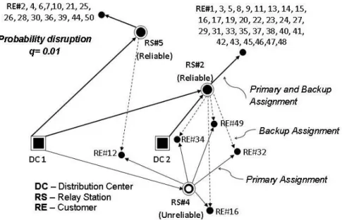
Results of MMA model are illustrated in Figures 3.4 and 3.5. We also showed it in Table 3.2 to compare the results among the model. From these, we know the DCs will distribute product to three open RSs for probability of disruption (qj) 0.01, 0.1, 0.2, 0.3 and 0.5 (RS#2, RS#4 and RS#5) in a multiple distribution manner. Except for q=0.4, two reliable RSs exist in the system. RS#4, which previously is unreliable RS, is eliminated in this probability. RS#4 turns to reliable ones when we increase the probability to 0.5.

In Figure 3.5 where q=0.5, all customers are assigned to RRS due to the increased probability of disruption. Though the opening RSs are same as the foregoing one, members of RS is different, and the distribution manner is considerably different with each other.

Chapter 3  

Figure 3.4: MMA model with disruption probability 0.01

Chapter 3  

Moreover, it is interesting to see that RS#4 is used as the unreliable RS when q is low while it is as the reliable one at the higher q after it disappears during the middle range of probability. This is because the opening cost of RS#4 is quite cheap among RSs. Hence, opening this RS as URS can save the transportation cost greatly when q is low. In contrast, when q becomes higher, it makes sense to open this RS as RRS to cope with the disruption as well as transportation