Tikhonov Regularization as a Complexity Measure
in Multiobjective Genetic Programming
Ji Ni and Peter Rockett
Abstract—We propose using Tikhonov regularization in con-junction with node count as a general complexity measure in multiobjective genetic programming. We demonstrate that employing this general complexity yields mean squared test error measures over a range of regression problems which are typically superior to those from conventional node count (but never statistically worse). We also analyze the reason why our new method outperforms the conventional complexity measure and conclude that it forms a decision mechanism which balances both syntactic and semantic information.
Index Terms—Genetic programming, Tikhonov regularization, Complexity measure, Pareto dominance.
I. INTRODUCTION
T
HE empirical modeling of data [1] has wide application in science, engineering, commerce and other related areas. Given some sample of n training data, D taken from anN-dimensional measurement space assumed drawn from a stationary distribution:D={x17→y1, . . .xn7→yn}wherexi∈RN, yi∈R a human data analyst would identify a family of likely regres-sion models (from an infinity of possible models) and perform the iterative sequence of: training (or calibration) to determine the optimal parameters followed by a diagnostic test on the adequacy of the model’s predictions. One of the key issues in empirical data fitting ismodel selection, determining which structural model form gives the most reliable predictions. Too simple a model will fail to capture the variability in the data (underfitting) while too complex a model will display spurious variability (overfitting). Bishop [2] shows a nice example of this dilemma in terms of polynomial functions. How to balance closeness-of-fit to the training set (which can usually be reduced by fitting a more complex model) against model complexity, is the essence of the model selection problem. This is commonly addressed by a regularization approach where the data analyst seeks the model with lowest value of:
E=Closeness-of-fit+λ×Complexity (1) where λ is the regularization constant and “Complexity” is some measure of the complexity of the model under consid-eration. In regression problems, “Closeness-of-fit” is normally mean squared error (MSE). Regularization is the basis of the well-known Akaike information criterion [3] as well as having J. Ni and P. Rockett are with the Department of Electronic and Electrical Engineering, University of Sheffield, Mappin Street, Sheffield S1 3JD, UK e-mail: [email protected]
Manuscript received August 7, 2012; revised —.
more general interpretation [4]; Bayesian model selection methods can often be interpreted in a regularization framework where a log prior forms the right-hand term in (1).
In essence, eqn. (1) expresses the trade-off between the desire to make the model fit the training data as closely as possible, and the competing desire to have as simple a model as possible to conform to the principle of parsimony, or Occam’s razor. Unfortunately, for some given data set and a given model, selecting λis not trivial since its value influ-ences the minimum of (1) and therefore the model selection decision. When regularization is used in the form of (1), cross validation schemes are often used to select λ. Alternatively, the regularization framework can be expressed as the simul-taneous desires to minimize the fitting error and the model complexity, which leads naturally to Pareto optimization in which identifying a specific, optimum value of λis avoided. Given some 2-vector of objectives f, where the elements of f are (i) the MSE over the training set, and (ii) a measure of model complexity, the Pareto dominance relation that an objective vector fi dominates fj (expressed symbolically as fi≺fj) is:
fi≺fj ,∀(k∈ {1,2};fki≤fkj)
∧ ∃(k∈ {1,2};fki< fkj) (2) What results from such a multiobjective optimization is a set of non-dominated individuals which delineate the fundamental trade-off between training-set MSE and model complexity. In the present context, we perform this multiobjective optimiza-tion1 using genetic programming (GP) [5] and obtain a set of candidate models which have the property that no models exist which are both less complex and have a lower training-set MSE. Analogous to the final model selection by a human data analyst discussed above, it remains to select one of the Pareto set of non-dominated models as the final model using an independent test set. The overarching advantage of the GP process, of course, is that GP is able to explore a far wider and richer set of possible model structures than can generally be considered by a human analyst.
A. Model Complexity
The foregoing is part background, part tutorial, that sets the scene for the remainder of the paper. Crucially, we have not so far discussed the key aspect of model complexity, how to measure the complexity of a quite general functional
1As is customary in the evolutionary literature, the term “optimize” is used
here to mean approximately optimal within the constraints of a stochastic algorithm.
model produced by GP. Multiobjective genetic programming (MOGP) was initially introduced [6] to address the bloat issue, the tendency of GP trees to increase in size without any accompanying improvement in performance. By imposing an evolutionary pressure to reduce tree size, bloated trees will be less likely to breed although we believe the situation is more subtle than this: simultaneously minimizing training set MSE and tree complexity is actually a regularization framework. Bloat control—which is the setting of some practical upper bound on tree size—follows as a beneficial consequence of regularization which principally seeks theleast complexmodel for some given training set MSE.
By far the most common complexity measure used to date in the MOGP literature is a count of the number of nodes in the GP tree. This was introduced because it was a “simple” and “easy to calculate” measure [6] although it is not without its philosophical difficulties. Firstly, it is a measure of the syntactic complexity of a tree. Considering the two expressions cos((3.2 + 0.8−1)x) and cos(9x) encoded as trees, the first appears twice as complex as the second despite being functionally smoother and therefore less likely to display excessive variability under prediction. In evolutionary breeding selection, the second tree would be preferred whereas from the perspective of evolving a function, the first is semantically simpler.
Second, every node in a tree contributes equally to a node count measure regardless of the function it implements. So a unary minus node and a sine transformation node are both equally weighted despite the sine node embedding an (infinite) power series which would intuitively appear more complex than a unary minus operation.
The apparent shortcomings of node count have motivated us to consider other complexity measures. Kolmogorov com-plexity [7] is known to be a fundamental measure although it is non-computable. Consequently, a number of other, more practical measures have been developed over the years. B. Tikhonov Regularization
In this paper we principally explore the use of Tikhonov regularizers in MOGP. Formally, Tikhonov regularization is defined [8], [9] in terms of the norm operator which broadly determines the ‘smoothness’ of a function. In a Sobolev space Wmp , the norm operator is given by:
||f||Wm p , Z |f|p+ ∂f ∂x p +. . . ∂mf ∂xm p dx p1 (3) wheremis the order of the regularizer andpis the norm. For the case ofp= 2(the Euclidean or 2-norm), a Sobolev space reduces to a Hilbert space, since Wm2 = Hm, and the norm operator is given by:
||f||Hm , " Z |f|2+ ∂f ∂x 2 +. . . ∂mf ∂xm 2! dx #12 = " m X k=0 ∂kf ∂xk 2 2 #12 (4)
wherek.k2 denotes the 2-norm.
Typically, regularization is applied by minimizing the so-calledTikhonov functional:
E=Eemp+λΩ (5)
where Eemp is the empirical error (typically mean squared error),λis the regularization constant andΩis the complexity term given by (4). The (lengthy) derivation of (4) can be found in [8], [9]. To calculate the regularizer for an m -times differentiable function we have to sum up to the m -th order partial derivatives of -the fitted function, which is usually approximated by a small number of low-order deriva-tives. Tikhonov regularization works by imposing additional constraints on the solution of the ill-posed learning problem in the form a ‘smoothness prior’ [9] but although smoothness is an intuitively obvious notion, expressing it mathematically is less straightforward. For example, the zeroth-order (m= 0) regularizer term in (4) tends to penalize functions with many extreme values whereas the first-order (m= 1) term disfavors functions which change rapidly. Wahba [10] informally noted that the second-order (m = 2) regularizer term penalizes the “wiggliness” of the fitted function (i.e., acts to suppress overfitting). Hence each term in (4) measures smoothness in a subtly different way.
From the perspective of GP, the regularizer in (4) is a semantic measure—that is, it is invariant to the particular syntax of a given GP tree. Furthermore, it has solid theoretical foundations.
C. Other Complexity Measures
In passing, and for completeness, we briefly discuss several other complexity measures that have been applied to GP.
Rissanen [11] introduced the Minimum Description Length (MDL) as a computable form of the Kolmogorov complexity and this was applied to GP by Iba et al. [12] who obtained neutral results. Reconsidering the two example mappings above,cos((3.2+0.8−1)x)andcos(9x), these two expressions ought to have the same MDL complexity measure but the first evaluates to be more complex than the second because it happens to be in non-minimal algebraic form. It is clear that just calculating the MDL from an unsimplified tree—as done by Iba et al.—only produces an upper bound on the MDL measure. The true MDL complexity measure of the tree can only be meaningfully computed, in the Kolmogorov sense, after the tree has been reduced to its minimal form, which, we suspect, is an NP-complete problem [13]. After numerical simplification, the above examples becomecos(3x) and cos(9x), with same MDL complexity measure (but the first expression is obviously smoother and has less ‘flexibility’ to overfit). We suspect that the failure to reduce their trees to minimal form explains the neutral results obtained in [12].
Second, Vladislavleva et al. [14] claim to have solved the model selection problem for GP by constructing a measure dependent on the order of the Chebyshev polynomials used to approximate the GP tree. In fact, careful inspection reveals that Vladislavleva et al. have converted the model selection problem in GP into a model selection problem on the set of
polynomial fits which they solve with an arbitrary threshold (their “” in the definition in Section B, [14, p. 337]). Thus they have not solved the GP model selection problem, rather changed it into another model selection problem which, in turn, they have not fundamentally solved.
Vanneschi et al. [15] proposed using the summation of partial complexity of each dimension inspired by the theory of generalized curvatures [16]. However, Vanneschi et al. did not show any evidence that such a measure yields superior test MSE. Further, curvature is one specific component of a Tikhonov regularizer—see (4). In addition, these authors used protected division in the their GP formulation and it is not clear how a second-order derivative was defined for this discontinuous function [17].
An interesting approach has been employed by Giustolisi and Savic [18] who define a set of pseudo-polynomial models where the inclusion/exclusion of terms in the model structure, and consequently the number of input variables, is determined by evolutionary search. In fact, [18] uses a genetic algorithm over a fixed-size chromosomal structure rather than genetic programming. The subsequent models—which can be “ex-tended” by incorporation of user-defined transformations—are (potentially) nonlinear in the input variables although linear-in-the-parameters, which are determined by conventional least-squares fitting. Giustolisi and Savic control the complexity2 of candidate models by placing an upper bound on the number of terms in the pseudo-polynomial; the number of terms used is one of the multiple objectives to be minimized. In fact, these authors implicitly employ a form of L0 regularization because omitting terms from the fitted function is equivalent to reducing an L0 norm—see (3)/(4) for the case when
p = 0 and m = 0. Overall, restriction of possible models to those belonging to a user-defined set is a limitation with the approach of [18].
The remainder of this paper is structured as follows: the next section presents the methodology to apply regularization to MOGP, and the statistical tests we have set up to assess the performance of the new method. Section III presents the development of our new complexity measure and the results obtained to support its superiority compared to node count. In Section IV we discuss the operation of regularization in MOGP and the reason for its success. Conclusions and future work is the last section of this paper.
II. METHODOLOGY
In this section we first discuss the implementation of regu-larization in MOGP followed by the development of a ‘grand complexity’ measure. The experimental methodology we have employed is covered in Section III.
2Giustolisi and Savic [18] use a different terminology to that used here.
In [18], the models contain no redundancy, unlike GP models, so these authors use the term “structural” complexity for what we refer to as “semantic” complexity. In this paper, “structural” complexity refers to the complexity of a GP tree which typically contains redundant nodes. “Semantic” complexity refers to the underlying mathematical transformation.
A. Implementation of Regularization
Except for the0-th order regularizer,m-th order regulariza-tion requires calcularegulariza-tion of the firstm (m= 1,2, ...) deriva-tives of the function. Therefore, all GP-generated individuals have be to analytic. Conventional (un)protected division can produce discontinuities [19] and lead to individuals which are non-differentiable. We consequently replaced conventional (un)protected division with ananalytic quotientoperator [17], defined in (6), to satisfy the condition of differentiability. Us-ing this analytic quotient systematically yields lower test MSE compared to conventional protected division and stabilizes the evolved trees by eliminating discontinuities. See [17] for more details. AQ(x1, x2) = x1 p 1 +x2 2 (6) Every individual evolved by GP is a tree which implicitly encodes a function. It is possible to transform such trees to evaluate a derivative of arbitrary order but for this initial exploratory study, we have estimated the necessary derivatives using numerical methods for convenience. In numerically computing derivatives, there is always a accuracy trade-off between rounding and truncation errors. We have used the method of Hahm et al. [20] who proposed the use of La-grange interpolation to approximate numerical derivatives and showed it to be superior to the widely-used central-difference method, achieving higher overall accuracy. For the numerical integration, we have used adaptive Gauss-Kronrod integration from the Gnu Scientific Library (GSL)3 to obtain a relative accuracy of10−6.
B. Application of Regularization with Extended Pareto-ranking
Regularization, having no regard to syntactic complexity, measures the ‘smoothness’ of a function which is a semantic measure. From Occam’s razor, we prefer simplerindividuals given the same MSE during the evolutionary process but there are, however, two difficulties with direct replacement of conventional node count by a regularizer in MOGP. One is that “simpler” needs not only to be interpretedsemanticallyto stabilize the model fit and produce smaller expected risk, but also syntacticallydue to the propensity of GP trees to bloat. Minimizing syntactic complexity will not necessarily minimize semantic complexity and vice versa (although these quantities will tend to exhibit some positive correlation). For example, a semantic complexity measure cannot distinguish between (x+2)and(x+2−1+1), preferring them equally, which is not desired. Semantic complexity cannot help to select trees with less syntactic redundancy. Similarly, a syntactic complexity measure cannot help to select variance-stabilized solutions.
The second practical difficulty with applying (semantic) regularization is that, even when the extra computational effort due to bloated trees is affordable, we will show in Sections III that a direct application of regularization causes premature convergence during the evolutionary process.
To cope with these two difficulties, we seek a complexity measure that minimizes both syntaxand semantic complexity simultaneously. An obvious approach is to use 3-dimensional MOGP to minimize MSE, node count and regularization simultaneously. Again we will show in Section III that prema-ture convergence still occurs. Moreover, syntactic and semantic complexities are not necessarily in competition with each other so treating them as independent objectives in a multiobjective optimization framework is probably not the best approach. A better, more cooperative strategy needs to be formulated between both complexity measures.
Reconsidering complexity, syntax and semantics are two components. As there is no easy way to combine them, we propose a 2-dimensional vector gthat consists of node count and regularizer to represent the general complexity of an in-dividual, and use Pareto comparison to select the simpler one. We term this 2D vector grand complexity as it reflects both the syntactic and semantic complexity of an individual. This selection method can handle the loose correlation between syntactic and semantic complexity and when the complexity of one individual dominates another, we have better confidence that that individual is ‘simpler’ and therefore to be preferred. Otherwise, we prefer neither individual as ‘simpler’ due to the contradictory evidence provided by syntax and semantics.
To apply this grand complexity to MOGP, we reformulate the traditional overall MOGP fitness vector into a fitness tuple that consists of: i) the MSE (∈R1), and ii) grand complexity, a two-dimensional vector which itself comprises node count (as a syntactic measure of bloat) and a regularizer (as a measure of solution smoothness). In general multiobjective optimization problems, the fitness vector consists of two or more objectives that are usually in conflict. Here we extend the fitness vector to afitness tuple, one component of which is a real number and the other a vector. The ranking method is an extension of the conventional Pareto comparison introduced by Goldberg [21]. In conventional Pareto-ranking, Goldberg [21] introduced assignment of equal ranks to all non-dominated individuals in a population so that non-dominated individuals within the same rank have the same probability to breed. For a minimization problem, recall from the definition in (2), for
n-dimensional vectors fi,j, an objective vector fi dominates fj iff:
fi≺fj ,∀(k∈ {1. . . n};fki≤fkj)
∧ ∃(k∈ {1. . . n};fki< fkj) (7) If an individual is not dominated by any other in the population, it is said to be non-dominated [21]. We denote the non-domination of fj by fi as fi ⊀fj. In (7), f is a real vector. We now expand this definition in a general sense by considering each component of the fitness tuple to be a vector rather than a real number.
Consider annmember fitness tupleG, each component of which is a ti-dimensional vector gwherei ∈ [1. . . n]. We define that Gj dominates Gk iff:
Gj≺Gk,∀(i∈ {1. . . n};gik⊀gij)
∧ ∃(i∈ {1. . . n};gij≺gik) (8) Similar to the case with (7), if Gj does not dominate Gk we consider Gk as non-dominated by Gj (Gj ⊀ Gk). If an individual is not dominated by any member of the population then it is said to be non-dominated. Notice that whengj,kare 1D vectors (i.e., scalars), (8) reduces to (7). With the extended definition of Pareto dominance in (8), we can address more complicated forms of comparisons, particularly when G comprises a scalar and a 2-vector. Considering specific examples where G1 = {M SE1,g1}, where g1 is the 2-vector comprising node count and a regularizer, and G2 ={M SE2,g2}, the extended Pareto comparison can be expressed in pseudo-C code in Algorithm 1.
Algorithm 1Algorithm for determining extended Pareto dom-inance if((M SE1< M SE2)and not(g2≺g1)) or((M SE1==M SE2)and(g1≺g2))then bDominated←true{G1≺G2} else bDominated←f alse{G1⊀G2} end if
C. Datasets and Experimental Protocol
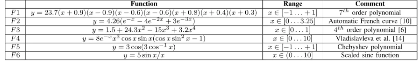
We have considered six one-dimensional regression prob-lems of varying degrees of curvature listed in Table I. We have generated 100 independent training sets from each function comprising 30 data, randomly-selected from the domain, and added zero-mean Gaussian noise with a variance of 0.01 to each training instance. Independent test sets comprising 100 000 randomly-drawn instances were used to assess gen-eralization performance.
Hastie et al. [22] remark that, given a large dataset, this should be split into: training, validation and test sets, where the validation set is used to select the final model, and the (independent) test set used to measure the generalization performance of the selected model. However, the practical situation [22] is that too few data are generally available to perform such a three-way split, and usual practice is to split the dataset into training and (disjoint) test sets4. Despite using
synthetic datasets, we have adopted an experimental protocol as close as possible to the practical compromise situation (although we have used a large test set to ensure an accurate test measure). In particular, we have conflated the validation and test phases to use the test set for both model selection from the final population, and estimation of the test error. This should be compared with the normal practice in single-objective GP (SOGP) where, typically, the best test error over multiple runs is reported. In essence, this selection over multiple SOGP runs is an implicit model selection stage, and entirely equivalent to the present protocol in an MOGP setting.
4Often, cross validation is used with repeated splits, but this option is not
TABLE I TESTFUNCTIONS
Function Range Comment
F1 y= 23.7(x+ 0.9)(x−0.9)(x−0.6)(x−0.6)(x+ 0.8)(x+ 0.4)(x+ 0.3) x∈[−1. . .+ 1] 7thorder polynomial
F2 y= 4.26(e−x−4e−2x+ 3e−3x) x∈[0. . .3.25] Automatic French curve [10]
F3 y= 1.5 + 24.3x2−15x3+ 3.2x4 x∈[0. . .1] 4thorder polynomial [6]
F4 y= 8e−xx3cosxsinx(cosxsin2x−1) x∈[0. . .10] Vladislavleva et al. [14]
F5 y= 3 cos(3 cos−1x) x∈[−1. . .+ 1] Chebyshev polynomial
F6 y= 5 sinx/x x∈(0. . .10] Scaled sinc function
Regardless, we have used the same assessment methodology for all cases so that the conclusions of the paper will be a fair comparison.
D. GP algorithms
To confirm that our conclusions are independent of evo-lutionary strategy, we have employed both generational GP with 50% elitism, and a steady-state algorithm. We have used rank-based selection for both strategies. For the steady-state experiments, we have used Pareto Converging Genetic Programming (PCGP), a GP adaptation of the multiobjective PCGA algorithm [23]. The strongly-elitist PCGA/P algorithm generates two offspring by crossover and mutation, which is always applied. These two new offspring are appended to the population, which is then re-ranked and the bottom-ranked two individuals discarded. The Pareto-converging algorithm was used in the present study since it has been shown to perform better than other, contemporary multiobjective evolutionary algorithms [24].
The GP parameters are summarized in Table II. The steady-state algorithm was run for 10 000 tree evaluations and the generational GP for an equivalent 198 generations. Note that these evaluations numbers only count a complete evaluation of a tree fitness, not the somewhat larger number of calculations necessary to perform the numerical differentiation/integration.
TABLE II
GP PARAMETERSUSED IN THISSTUDY
Population size 100
No. of evaluations (steady-state) 10 000 No. of evaluations (generational) 198
Crossover Point crossover [5] Mutation Point mutation [5]; Tree depth = 4
Node types Unary minus
Addition, Subtraction Multiplication Analytic quotient [17]
E. Experimental Setup
For each function, we have run paired statistical tests over 100 independent training sets by minimizing both MSE and complexity measure, which is either node count, regularizer or grand complexity. We have employed regularizers of either zeroth- (m= 0), first- (m= 1) or second-order (m= 2)—see (4)—to explore the performance over different ways of defin-ing smoothness. We computed statistics usdefin-ing the individual in the final population of each GP run with the lowest error over the relevant independent test sets described in Section II-C.
III. RESULTS
A. Direct Application of Regularization
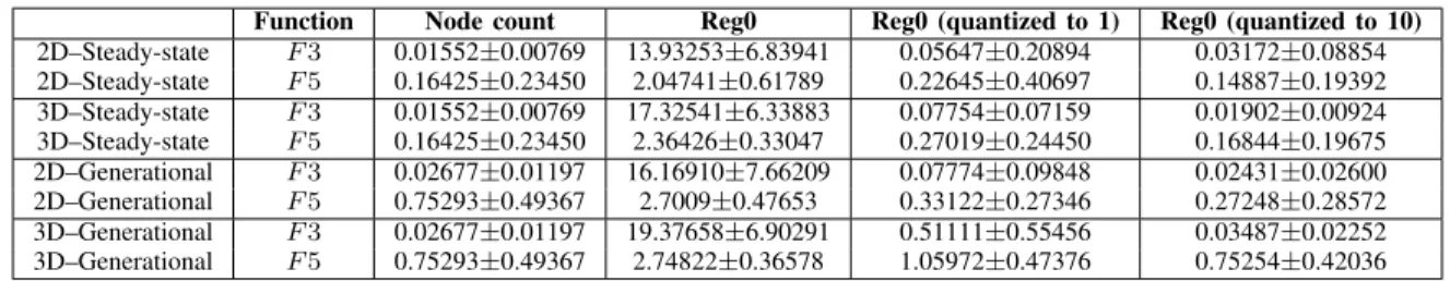
The results of directly applying zeroth-order regular-ization in MOGP are shown in Table III for both 2D (MSE/regularizer) and 3D objective vectors (MSE/node count/regularizer). For brevity we present only results for the
F3andF5 test functions which are quite typical. Comparing columns 3 (‘Node count’) and 4 (‘Reg0’) of Table III, it is obvious that the node count complexity measure produces significantly better average test errors. Inspection of the pop-ulations reveals that regularization has resulted in premature convergence—all individuals have quickly become all rank-1 thereby eliminating all selective pressure. This observation holds both for the 2D and 3D objective vectors. Clearly regularization on its own is worse than conventional node count.
Closer inspection shows that the premature convergence we observe using a regularization measure is due to a failure to maintain selective pressure in the population when using more than one real objective. Consider a non-dominated objective vector f = f1 f2
T
where f1,2 ∈ R. If we generate a new but marginally different individual with objective vector
f1+δ f2−δ T
, for some arbitrarily small δ, this too will be non-dominated. It is thus fairly easy to reduce the population to all rank-1 individuals by essentially resampling the existing rank-1 solutions rather than advancing the Pareto front. At this point all selective pressure ceases and this is indeed what we observe in practice.
To preserve effective selective pressure, and inspired by the idea of ε-dominance [25], we have experimented with quan-tizing the regularizer since ε-dominance increases selective pressure. The results of quantizing [replacing the regularizer Ω with Ω−(ΩmoduloQ) where Q = 1or 10] are shown in columns 5 and 6 of Table III. It is clear that quantization has improved the performance to be as good as node count in some cases, particularly for Q = 10, but still just worse than node count in others. After quantization, inspection of the populations revealed that premature convergence had either been eliminated (Q = 10) or at least delayed (Q = 1). Nonetheless, naive application of regularization—either as a replacement for node count in a 2D optimization, or in addition to it in a 3D formulation—produces no advantage in GP despite its theoretical solidity.
B. Grand Complexity
The test error performances over 100 repetitions for the grand complexity measure with zeroth, first and second order
TABLE III
2D-MOGP MEAN& STANDARDDEVIATION(SD)OF THE TESTMSEOVER FINAL POPULATION FOR DIFFERENT COMPLEXITY MEASURES(NODE COUNT,ZEROTH-ORDER REGULARIZATION,AND QUANTIZED ZEROTH-ORDER REGULARIZATIONS).
Function Node count Reg0 Reg0 (quantized to 1) Reg0 (quantized to 10)
2D–Steady-state F3 0.01552±0.00769 13.93253±6.83941 0.05647±0.20894 0.03172±0.08854 2D–Steady-state F5 0.16425±0.23450 2.04741±0.61789 0.22645±0.40697 0.14887±0.19392 3D–Steady-state F3 0.01552±0.00769 17.32541±6.33883 0.07754±0.07159 0.01902±0.00924 3D–Steady-state F5 0.16425±0.23450 2.36426±0.33047 0.27019±0.24450 0.16844±0.19675 2D–Generational F3 0.02677±0.01197 16.16910±7.66209 0.07774±0.09848 0.02431±0.02600 2D–Generational F5 0.75293±0.49367 2.7009±0.47653 0.33122±0.27346 0.27248±0.28572 3D–Generational F3 0.02677±0.01197 19.37658±6.90291 0.51111±0.55456 0.03487±0.02252 3D–Generational F5 0.75293±0.49367 2.74822±0.36578 1.05972±0.47376 0.75254±0.42036 TABLE IV
MEAN& SDOF TESTMSEOVER FINAL POPULATION FOR STEADY-STATEMOGPFOR DIFFERENT COMPLEXITY MEASURES(NODE COUNT AND GRAND COMPLEXITY OF VARIOUS ORDERS). THE STATISTICALLY SIGNIFICANT DIFFERENCES COMPARED TO NODE COUNT AT THE95%CONFIDENCE ARE
SHOWN IN BOLD.
Node count GrC-Reg0 GrC-Reg1 GrC-Reg2
F1 0.07613±0.01963 0.07208±0.02767 0.07592±0.02683 0.07622±0.02590 F2 0.00992±0.00594 0.01087±0.00958 0.01056±0.00750 0.01117±0.00774 F3 0.01552±0.00769 0.01246±0.01020 0.01036±0.00942 0.01106±0.00927 F4 3.87450±0.73913 3.54921±1.19285 3.55683±1.21241 3.56018±1.01944 F5 0.16425±0.23450 0.14361±0.21993 0.12255±0.16456 0.11850±0.18722 F6 0.23677±0.08802 0.25021±0.16537 0.22958±0.18239 0.17243±0.10550 TABLE V
MEAN& SDOF TESTMSEOVER FINAL POPULATION FOR GENERATIONALMOGPFOR DIFFERENT COMPLEXITY MEASURES(NODE COUNT AND GRAND COMPLEXITY OF VARIOUS ORDERS). THE STATISTICALLY SIGNIFICANT DIFFERENCES COMPARED TO NODE COUNT AT THE95%CONFIDENCE ARE
SHOWN IN BOLD.
Node count GrC-Reg0 GrC-Reg1 GrC-Reg2
F1 0.08957±0.01653 0.08727±0.02495 0.08514±0.01978 0.08675±0.02073 F2 0.01423±0.00601 0.01431±0.01103 0.01215±0.00856 0.01257±0.00810 F3 0.02677±0.01197 0.02168±0.01769 0.01820±0.01134 0.02258±0.01719 F4 4.52316±0.52974 4.21823±0.66818 4.15471±0.61496 4.10144±0.73548 F5 0.75293±0.49367 0.23714±0.29356 0.30099±0.25286 0.40635±0.35568 F6 0.35633±0.10727 0.27558±0.12428 0.29139±0.13742 0.27716±0.16983
regularizers are shown in Table IV for steady-state evolution, and Table V for the generational algorithm. Generally, grand complexity gives a lower mean test error than using node count with the exception of test function F2 for the steady-state method. As far as we have observed, there does not appear to be a great deal of difference between the different-order regularizers.
To further examine the significance of the results in Ta-bles IV and V, we have performed a one-sided paired sign-test under the null hypothesis that the median difference between the two methods is≤0[26]. If grand complexity outperforms node count in ≥ 59 pairwise comparisons then this implies statistical significance at the 95% confidence level. Conversely, if grand complexity is outperformed by node count in ≤ 41 comparisons, this implies node count is statistically superior at the 95% level. The outcomes of the pairwise comparisons are shown in Tables VI and VII for steady-state and generational algorithms, respectively together with the corresponding p -values. In 25 of the 36 comparisons, grand complexity is statistically superior, sometimes at the 99.99% confidence level. In the remaining eleven comparisons, there is no strong evidence to support the superiority of either method. Most significantly, in no case is node count statistically superior.
(From the foregoing, it might be inferred that the gen-erational algorithm is superior. Directly performing pairwise
TABLE VI
SIGN TEST RESULTS COMPARINGGRCWITH DIFFERENT REGULARIZERS, AGAINST NODE COUNT;STEADY-STATE. THE‘+’COLUMN SHOWS THE NUMBER OF TIMES OUT OF100TRIALS THATGRCGAVE A SMALLER TEST
ERROR THAN NODE COUNT.
Reg 0 Reg 1 Reg 2
+ p-Value + p-Value + p-Value F1 60 0.0228 51 0.4207 52 0.3446 F2 49 0.5793 46 0.7881 46 0.7881 F3 69 0.0001 75 <10−4 74 <10−4 F4 56 0.1151 53 0.2743 64 0.0026 F5 59 0.0359 53 0.2743 59 0.0359 F6 50 0.5000 58 0.0548 76 <10−4
comparisons between the corresponding steady-state and gen-erational results shows that the steady-state PCGP algorithm consistently outperforms the generational algorithm at the ≥99.99% confidence level. So although grand complexity in the generational algorithm scores more successes over node count than for PCGP, this is because the strongly elitist, steady-state PCGP algorithm with node count produces better results than the generational/node count combination; grand complexity in the generational algorithm thus has a weaker set of ‘opponents’ to beat in the pairwise tests. This observation of the superiority of the steady-state algorithm reinforces our previous observations, for example [24].)
TABLE VII
SIGN TEST RESULTS COMPARINGGRCWITH DIFFERENT REGULARIZERS, AGAINST NODE COUNT;GENERATIONAL EVOLUTION. THE‘+’COLUMN SHOWS THE NUMBER OF TIMES OUT OF100TRIALS THATGRCGAVE A
SMALLER TEST ERROR THAN NODE COUNT.
Reg 0 Reg 1 Reg 2
+ p-Value + p-Value + p-Value F1 62 0.0082 63 0.0047 61 0.0139 F2 58 0.0548 68 0.0002 62 0.0082 F3 66 0.0007 70 <10−4 63 0.0047 F4 73 <10−4 78 <10−4 75 <10−4 F5 81 <10−4 78 <10−4 75 <10−4 F6 74 <10−4 74 <10−4 79 <10−4 IV. DISCUSSION
To further explore the reason for the superiority of grand complexity, we analyzed the properties of MOGP with grand complexity compared to the other methods of computing a complexity measure.
A. Premature Convergence of Regularization
Based on regularization theory, we seek to minimize (5). Minimizing MSE and complexity simultaneously will effec-tively minimize the Tikhonov functional and should yield a set of non-dominated rank-1 individuals with various (implicit) values of λ. In other words, theoretically it is possible to minimize MSE/complexity using MOGP to yield a set of individuals with the lowest attainable MSE for some given value of Ω. Based on our experiments, however, GP in such a setting suffers premature convergence in that the whole population converges to all rank-1 individuals at a very early stage and the MSE remains large due to stagnated search. Cru-cially, this premature convergence is not a failing of Tikhonov regularization, rather a problem caused by the interaction of two, real-valued objectives in MOGP.
Regularization concerns only the semantic ‘smoothness’ of a function without any regard to its syntactic representation so it is not surprising that GP, as a syntax-based algorithm, experiences problems with no control on its syntax. We have tried using a 3D objective vector within MOGP, minimizing MSE/node count/regularizer, however, premature convergence remains. Premature convergence leads to all rank-1 individuals and causes the evolution to degenerate to random search, which is the reason for the low efficiency.
To further study the reason why premature convergence oc-curs, we have inspected the properties of the newly-generated offspring. As premature convergence can be considered as a rapid growth in the numbers of individuals labeled as rank-1 (regardless of their absolute quality), we recorded the Pareto comparison between the newly-generated offspring and the current rank-1 individuals. (Here “current” is taken as the quasi-stationary population in the case of steady-state evolution, and the existing population from which offspring are being generated in the case of the generational model.) We can identify three mutually-exclusive outcomes from such a comparison:
i) The new offspring dominates at least one individual on the current Pareto-front. The Pareto front is thus
advanced, and the number of rank-1 individuals will not increase.
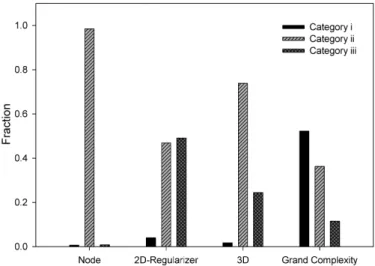
ii) The new offspring is dominated by the current Pareto front. The offspring will be labeled as of lower than rank-1, hence making no impact on the Pareto-front. iii) The new offspring is neither of (i) nor (ii). In this situation, the new individual is labeled as rank-1 and the number of rank-1 individuals will be increased. The Pareto-front thus expands rather than being advanced. Note that this outcome is the main cause of the population converging to all rank-1 individuals. The probability of each category is obtained straightfor-wardly from the counts of offspring falling into each category divided by the total number of newly generated offspring. We accumulated the statistics over 100 training sets and characterized the average value of the probabilities in each category. Since regularizers with different orders give similar results, we present results only for the0-th-order regularizer. The results are summarized in Figs. 1 and 2 for test functions
F2andF5.
For the node count complexity objective, it is very rare for offspring to fall to categories (i) and (iii), as most fall to (ii). This implies that it is rare for node count to generate a new rank-1 individual either by improving or expanding the current Pareto-front. With a low rate of Pareto-front expansion, the evolutionary process using node count remains stable and yields good results, albeit rather slowly and, by implication, inefficiently.
For 2D and 3D MOGP minimizing MSE vs. regularizer, and MSE vs. regularizer vs. nodes, respectively, both methods have small probabilities of generating category (i) individuals, while category (iii) offspring are much more likely than category (i). This means that there is large chance that the newly-generated individuals will be rank-1 but most are simply supplementing the current Pareto-front rather than improving it. If the popula-tion is of all rank-1 individuals, then optimizapopula-tion is reduced to simple random search and hence is very inefficient. We believe this is the reason why both 2D and 3D MOGP suffer premature convergence.
Fig. 1. Mean value of probabilities of generating category (i), (ii) and (iii) outcomes for test functionF2.
Fig. 2. Mean value of probabilities of generating category (i), (ii) and (iii) outcomes for test functionF5.
For grand complexity, the probability of generating category (iii) individuals that fill-in the Pareto-front is lower than for 2D and 3D, however it is still much higher than for node count. The reason that grand complexity does not suffer premature convergence despite generating large numbers of category (iii) individuals is that grand complexity also generates an even higher number of category (i) individuals. Such individuals keep driving the Pareto front forward and mitigate the category (iii) individuals by dominating them, thereby reducing them to lower ranks. Thus under grand complexity, the population does not prematurely converge to all rank-1 individuals.
To gain further insight into how the ranking distribution changes during evolution, Fig. 3 shows the maximum ranks during the evolutionary processes starting from an identical initial population for test function F3. In Fig. 3, grand complexity starts from large maximum rank—more than 60 on initialization—and keeps the maximum rank fluctuating over all the 10 000 evaluations.
The maximum rank for node count starts from a little over 20, and reduces quickly to lower value but certainly larger than unity, thereby stably maintaining evolutionary pressure. The rank range of 3D MOGP starts from less than 20 and quickly reduces to one, which indicates a premature convergence. With exactly the same initial population, three choices of complexity objective thus lead to significantly different ranking results. The greater ability of grand complexity to maintain individuals over a more diverse range of ranks makes it less likely to prematurely converge, as well as preserving evolutionary pressure. Neither node count nor grand complexity suffers from premature convergence but the higher rank diversity in grand complexity exerts greater evolutionary pressure and tends to yield fitter elite individuals.
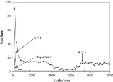
Fig. 4 compares 2D regularization with different quantiza-tions again for test functionF3and illustrates how a quantized regularizer affects premature convergence. For the original, unquantized regularizer, the maximum rank starts at a little less than 40 (higher diversity compared to node count) but reduces very quickly. Occasionally in the remainder of the 10 000 iterations the maximum rank increases to 2 or 3, but
Fig. 3. Maximum ranks as a function of iteration number for: 3D MOGP, node count and grand complexity measures; steady-state evolution.
returns to 1 very rapidly. With exactly the same algorithm and initialization, quantizing the regularization measure,Ω→
[Ω−(Ωmodulo1)]has a larger range of ranks on initialization and delays degeneration to all rank-1 individuals until around 2000 iterations.
Fig. 4. Maximum ranks as a function of iteration number for0-th order regularizer, and with quantizations of Q = 1and Q = 10; steady-state evolution.
Quantizing the regularizer as [Ω−(Ωmodulo10)] further improves the rank distribution and maintains a better spread of ranks throughout the whole evolutionary process. In other words, a properly quantized regularizer may have the potential to produce good performance. From Fig. 5, it is easy to see how three individuals which are all rank-1 in continuous regularization space take on a range of ranks from 1 to 3 after quantization (i.e., projected onto the vertical dashed line). Quantization increases the range of ranks and thereby prevents premature convergence. However, determining the quantization scale Q is problem-dependent and there seems no way to predetermine it other than enumerative search. Moreover, despite careful tuning of the quantization, the
Fig. 5. Illustration of the way quantization of the regularization measure increases rank diversity. Three individuals all of rank-1 are quantized to ranks-1 to 3.
improvement compared to node count is small; we observe no result better than node count even where highly diversified ranks are maintained by quantizing the regularizer. This shows that the high rank diversity is a necessary but not sufficient condition for better results. The regularizer quantized to 10 provides wider rank diversity than node count (cf. Figs. 3 and 4), however, the elite individuals evolved under the higher selective pressure from quantized regularizer are not as good as those evolved with lower pressure from node count. This phenomenon implies that not all the superiority of grand complexity over node count is due to maintaining a higher rank diversity and higher evolutionary pressure, but that grand complexity forms an intrinsically better general complexity measure.
B. Pareto Comparison of Grand Complexity
An interesting aspect of grand complexity is that it is very similar to 3D MOGP but the evolutionary processes clearly differ significantly. Table VIII lists the two comparisons in detail. In this table, the comparisons between MSE values are shown horizontally and those based on the grand complexity vector components are shown vertically. Based on Goldberg’s algorithm, there is a binary relation between two individuals ‘A’ and ‘B’. ‘A’ either dominates ‘B’ (denoted by ‘D’), or ‘B’ is not dominated by ‘A’ (denoted by ‘ND’).
From Table VIII, there are only two cases where 3D Pareto comparison and grand complexity produce different results, indicated by the grayed cells. Taking the first of these cases for illustration, despite the fact that ‘A’ has a lower MSE than ‘B’ and a smaller node count, its regularizer is larger. Thus under 3D vector comparison, ‘A‘ does not dominate ‘B’ as there is no clear evidence to indicate the superiority of either individual. For grand complexity, the opposing relations
TABLE VIII
GRAND COMPLEXITY(GRC)AND3DRELATIONS. THE DIFFERENCES ARE HIGHLIGHTED IN GRAY. MSE Complexity < = > Node # Regularizer GrC 3D GrC 3D GrC 3D < < D D D D ND ND < = D D D D ND ND < > D ND ND ND ND ND = < D D D D ND ND = = D D ND ND ND ND = > ND ND ND ND ND ND > < D ND ND ND ND ND > = ND ND ND ND ND ND > > ND ND ND ND ND ND
between node count (‘<’) and regularizer (‘>’) mean thatgA will not dominategB so the overall result of the comparison will be determined by the relative MSEs. Thus under grand complexity, ‘A’ does indeed dominate ‘B’. Grand complexity effectively reduces the syntactic and semantic complexity to a lower priority compared to MSE and forms a ‘soft’ decision in terms of complexity.
As to the impact on the behavior of GP, based on Figs. 1 and 2, we believe this is the reason that grand complexity produces a higher probability of generating better, category (i) individuals compared to 3D MOGP. This small difference essentially improves the evolutionary process from one prone to premature convergence to one with a stable population.
Finally, for future work, it is worth considering transforma-tion of trees to yield the derivative of the tree functransforma-tion rather than using numerical differentiation. This would involve a fairly straightforward recursive application of the laws of basic calculus and save significant computing time, especially for extension to higher-order regularizers and higher-dimensional problems.
V. CONCLUSIONS
In this paper, we propose applying Tikhonov regulariza-tion, a general semantic complexity (smoothness) measure, in MOGP. We extend Pareto-ranking between vectors to tuples, constructing a general complexity measure,grand complexity, that incorporates both the syntactic and semantic complexities of individuals. Grand complexity with regularizers of different orders yields generally lower test mean squared errors; we have confirmed our observations with appropriate statistical sign tests. Further, we have examined the mechanisms why grand complexity outperforms node count and shown that whereas the node count complexity measure leads to large fractions of offspring which are dominated by existing popula-tion members, grand complexity is able to produce significant numbers of offspring which advance the Pareto front. Grand complexity maintains a larger range of ranks and thus sustains a high selective pressure. In addition, using regularization alone leads to premature convergence. We conclude that grand complexity forms a ‘soft’ comparison able to incorporate the non-commensurate syntactic and semantic complexity mea-sures and is thus a superior complexity measure.
REFERENCES
[1] G. E. P. Box and N. R. Draper,Empirical Model-building and Response Surfaces. New York: Wiley, 1987.
[2] C. M. Bishop, Neural Networks for Pattern Recognition. Oxford: Clarendon Press, 1995.
[3] H. Akaike, “A new look at the statistical model identification,”IEEE Trans. Autom. Control, vol. 19, no. 6, pp. 716–723, 1974.
[4] V. N. Vapnik,The Nature of Statistical Learning Theory,2nded. New
York: Springer, 2000.
[5] R. Poli, W. B. Langdon, and N. F. McPhee,A Field Guide to Genetic Programming. Published via http://lulu.com and freely available at http://www.gp-field-guide.org.uk, 2008.
[6] A. Ek´art and S. Z. N´emeth, “Selection based on the Pareto nondomi-nation criterion for controlling code growth in genetic programming,”
Genet. Program. Evol. M., vol. 2, no. 1, pp. 61–73, 2001.
[7] T. M. Cover and J. A. Thomas,Elements of Information Theory,2nded.
Hoboken, N.J.: John Wiley, 2006.
[8] A. N. Tikhonov and V. Y. Arsenin, Solutions of Ill Posed Problems. Washington, D.C: V.H.Winston, 1977.
[9] Z. Chen and S. Haykin, “On different facets of regularization theory,”
Neural Comput., vol. 14, no. 12, pp. 2791–2846, 2002.
[10] G. Wahba,Spline Models for Observational Data. Philadelphia, PA: Society for Industrial and Applied Mathematics, 1990, vol. 59. [11] J. Rissanen, “Modeling by shortest data description,” Automatica,
vol. 14, no. 5, pp. 465–471, 1978.
[12] H. Iba, H. de Garis., and T. Sato, “Genetic programming using a minimum description length principle,” in Advances in Genetic Pro-gramming. MIT Press, 1994, pp. 265–284.
[13] M. R. Garey and D. S. Johnson,Computers and Intractability: A Guide to the Theory of NP-completeness. San Francisco, CA: W. H. Freeman, 1979.
[14] E. J. Vladislavleva, G. F. Smits, and D. den Hertog, “Order of nonlinear-ity as a complexnonlinear-ity measure for models generated by symbolic regression via Pareto genetic programming,”IEEE Trans. Evol. Comput., vol. 13, no. 2, pp. 333–349, 2009.
[15] L. Vanneschi, M. Castelli, and S. Silva, “Measuring bloat, overfitting and functional complexity in genetic programming,” in 12th Annual Conference on Genetic and Evolutionary Computation (GECCO ’10), Portland, OR, 7-11 July 2010, pp. 877–884.
[16] J.-M. Morvan,Generalized Curvatures. Berlin: Springer, 2008. [17] J. Ni, R. H. Drieberg, and P. I. Rockett, “The use of an analytic quotient
operator in genetic programming,”IEEE Trans. Evol. Comput., vol. 17, no. 1, pp. 146–152, 2013.
[18] O. Giustolisi and D. A. Savic, “Advances in data-driven analyses and modelling using EPR-MOGA,”J. Hydroinform., vol. 11, no. 3-4, pp. 225–236, 2009.
[19] M. Keijzer, “Improving symbolic regression with interval arithmetic and linear scaling,” inEuropean Conference on Genetic Programming (EuroGP 2003), Essex, UK, 2003, pp. 70–82.
[20] N. Hahm, M. Yang, and B. I. Hong, “Generalized numerical differentia-tion using the Lagrange interpoladifferentia-tion,”J. Appl. Math. Comput., vol. 21, no. 1/2, pp. 495–504, 2006.
[21] D. E. Goldberg,Genetic Algorithms in Search, Optimization and Ma-chine Learning. Reading, MA: Addison Wesley, 1989.
[22] T. Hastie, R. Tibshirani, and J. Friedman, The Elements of Statistical Learning: Data Mining, Inference, and Prediction,2nded.
Springer-Verlag, 2009.
[23] R. Kumar and P. I. Rockett, “Improved sampling of the Pareto-front in multiobjective genetic optimizations by steady-state evolution: A Pareto converging genetic algorithm,”Evol. Comput., vol. 10, no. 3, pp. 283– 314, 2002.
[24] Y. Zhang and P. I. Rockett, “Comparison of evolutionary strategies for multi-objective genetic programming,” in IEEE Systems, Man & Cybernetics Society Conference on Advances in Cybernetic Systems (AICS2006), Sheffield, UK, 2006.
[25] M. Laumanns, L. Thiele, K. Deb, and E. Zitzler, “Combining conver-gence and diversity in evolutionary multiobjective optimization,”Evol. Comput., vol. 10, no. 3, pp. 263–282, 2002.
[26] P. Sprent and N. C. Smeeton,Applied Nonparametric Statistical Meth-ods,4thed. London / Boca Raton, FL: Chapman and Hall/CRC, 2007.