Upland vegetation mapping using Random Forests with
optical and radar satellite data
Brian Barrett1, Christoph Raab2, Fiona Cawkwell3& Stuart Green4
1School of Geographical and Earth Sciences, University of Glasgow, Scotland, United Kingdom 2Centre of Biodiversity and Sustainable Land Use, University of G€ottingen, Gottingen, Germany€ 3School of Geography and Archaeology, University College Cork (UCC), Cork, Ireland
4Teagasc, Irish Agriculture and Food Development Authority, Ashtown Dublin 15, Dublin, Ireland
Keywords
Radar, random forests, remote sensing, satellite data, uplands, vegetation mapping Correspondence
Brian Barrett, School of Geographical and Earth Sciences, University of Glasgow, Scotland, UK. Tel: +44 (0)141 330 8655; Fax: +44 (0)141 330 4817;
E-mail: [email protected] Funding Information
This research was funded by the
Environmental Protection Agency (Ireland) as part of the Science, Technology, Research and Innovation for the Environment (STRIVE) Programme 2007–2013.
Editor: Harini Nagendra Associate Editor: Ned Horning Received: 8 July 2015; Revised: 22 September 2016; Accepted: 27 September 2016
doi: 10.1002/rse2.32
Abstract
Uplands represent unique landscapes that provide a range of vital benefits to society, but are under increasing pressure from the management needs of a diverse number of stakeholders (e.g. farmers, conservationists, foresters, govern-ment agencies and recreational users). Mapping the spatial distribution of upland vegetation could benefit management and conservation programmes and allow for the impacts of environmental change (natural and anthropogenic) in these areas to be reliably estimated. The aim of this study was to evaluate the use of medium spatial resolution optical and radar satellite data, together with ancillary soil and topographic data, for identifying and mapping upland vegetation using the Random Forests (RF) algorithm. Intensive field survey data collected at three study sites in Ireland as part of the National Parks and Wild-life Service (NPWS) funded survey of upland habitats was used in the calibra-tion and validacalibra-tion of different RF models. Eight different datasets were analysed for each site to compare the change in classification accuracy depend-ing on the input variables. The overall accuracy values varied from 59.8% to 94.3% across the three study locations and the inclusion of ancillary datasets containing information on the soil and elevation further improved the classifi-cation accuracies (between 5 and 27%, depending on the input classificlassifi-cation dataset). The classification results were consistent across the three different study areas, confirming the applicability of the approach under different envi-ronmental contexts.
Introduction
Regular monitoring of vegetation in upland areas is important for biodiversity conservation, land manage-ment, carbon storage and within a European context, European Union (EU) policy compliance. Approximately 19% of the area of the Republic of Ireland supports upland habitats and these have not been adequately described or their distribution adequately mapped (Perrin et al. 2009). These upland areas contain the nation‘s
largest expanse of semi-natural habitats and provide many
benefits to society – water supply, climate regulation,
maintenance of biodiversity, and provision of recreational activities to name but a few. Notwithstanding this, the uplands are under increasing pressure from a myriad of issues; grazing management, scrub encroachment, dimin-ished supports, ageing farming population and abandon-ment of land that will lead to major landscape changes into the future (MacDonald et al. 2000; Reed et al. 2009). These stresses have serious consequences upon the
composition, extent and conservation status of important vegetation habitats in these areas (Mehner et al. 2004). The inaccessibility and scale of the uplands, along with constraints in time and finance, make monitoring changes in vegetation covering large spatial areas difficult using traditional field-based surveys (Lees and Ritman 1991; Buchanan et al. 2005; Rhodes et al. 2015). The use of Earth Observation (EO) data can help overcome this problem (Kerr and Ostrovsky 2003; Gillespie et al. 2008; Vanden Borre et al. 2011) and help comply with report-ing obligations under the Birds Directive (Council Direc-tive 79/409/EEC 1979) and the Habitats DirecDirec-tive (Council Directive 92/43/EEC 1992). The number of EO satellites orbiting the Earth is increasing, and concurrent with algorithmic advances in information extraction capa-bilities (Lausch et al. 2015), EO datasets offer a real possi-bility to provide reliable, high-quality and spatially explicit maps of habitat distribution and monitor habitat fragmentation at intervals determined by management needs (Nagendra et al. 2013; Barrett et al. 2014; Pettorelli et al. 2014a).
In order to obtain sufficient information at the ecotope level, hyperspectral data can be the preferred choice in some studies and has been successfully demonstrated under various conditions (Lawrence et al. 2006; Chan and Paelinckx 2008; Chan et al. 2012; Delalieux et al. 2012; Lucas et al. 2015). However, hyperspectral data is not always or commonly available, and in its absence, multi-spectral data have also shown their use for habitat map-ping (e.g. Feilhauer et al. [2014] and Corbane et al. [2015]). The difficulty of acquiring cloud-free observa-tions in temperate areas prone to persistent cloud cover-age, especially during spring and summer periods often limits the capability of classifying habitats with optical data as it is not possible to capture the seasonal variability in the spectral response of the vegetation (Lucas et al. 2011). Additionally, upland areas are usually more prone to cloud cover due to the effects of orographic lift. Con-sequently, Synthetic Aperture Radar (SAR) data are increasingly being investigated for landscape monitoring as they are largely unaffected by atmospheric conditions (Baghdadi et al. 2009; Waske and Braun 2009; Evans and Costa 2013; Barrett et al. 2014). SAR data are sensitive to vegetation structure and moisture content and in combi-nation with optical data, may help to further improve discrimination of habitats that are structurally different but spectrally similar.
The choice and availability of suitable EO data will ulti-mately determine the amount of information that can be extracted to map and monitor habitats to varying degrees of resolution. In general, most studies are concerned with using the highest spatial resolution data possible, which often introduces further challenges in terms of the
maximum coverage that is attainable and financial con-straints in acquiring the data. In many cases, extremely detailed imagery may not be needed for a widespread conservation status assessment and the use of medium
spatial resolution (>10 and≤20 m) data may be sufficient
to capture the broad extent and spatial patterns of habi-tats and meet the local needs of stakeholders along with national requirements in terms of reporting under the EU Directives (Lucas et al. 2007; Varela et al. 2008; Nagendra et al. 2013). Within this context, the objective of this study is to evaluate the use of medium spatial resolution optical and radar satellite data, together with ancillary soil and topographic data for identifying and mapping upland vegetation to complement field studies and help con-tribute to national policy in the area of upland manage-ment and the future sustainable developmanage-ment of the uplands. The definition used in this study for upland habitats is taken from Perrin et al. (2009) and is the same as that used by the NPWS of Ireland, whereby uplands are defined as unenclosed areas of land over 150 m in ele-vation, and contiguous areas of related habitats that des-cend below this value. Consequently, the study also includes areas below the 150 m cut-off to include the broad band of transitional vegetation and land manage-ment that exists between lowland and upland habitats.
Materials and Methods
Study sites
Suitable study areas were selected from a list of candidate sites for an upland monitoring network, proposed by Per-rin et al. (2009) that is designed to meet part of Ireland‘s obligations under Articles 6, 11 and 17 of the Habitats Directive (92/43/EEC). Figure 1 displays the three areas selected for this study; Mount Brandon, the Galtee Moun-tains, and the Comeragh Mountains.
Mount Brandon
Mount Brandon is located on the Dingle Peninsula in west Kerry, in south western Ireland. It is a mountainous
area that includes the second highest peak in Ireland –
Mount Brandon at 952 m. It is a designated candidate Special Area of Conservation (cSAC 000375, Lat: 52.22,
Long:10.07) and the area has an oceanic climate with a
mean temperature range of between 7 and 13°C and a
mean annual rainfall of 1560 mm (calculated from the
1981–2010 averages of the nearest synoptic weather
sta-tion at Valentia), although the upland summits often receive over 3000 mm per annum. The area of the
stud-ied upland site is 162 km2 (16,212 ha) while the area of
Galtee Mountains
The Galtee Mountains span across three counties: Cork, Tipperary and Limerick, and are the highest inland mountain range in Ireland (Galtymore at 920 m). It is a designated candidate Special Area of Conservation (cSAC
000646, Lat: 52.36, Long: 8.14), where the mean
recorded temperature range is 5–13°C with a mean
annual precipitation of 820 mm for the lowlands, rising to 1900 mm for upland regions (meteorological data recorded at the closest synoptic weather station at Moore-park in Fermoy, Cork). The area of the studied upland
site is 83 km2 (8279 ha) while the area of the entire
region in Figure 1(B) is 619 km2.
Comeragh Mountains
The Comeragh Mountains are located in county Water-ford and are a designated Special Area of Conservation
(SAC 001952, Lat: 52.23, Long: 7.56). The central area
of the mountains features a boggy plateau and reaches a maximum elevation of 792 m. Moorepark is also the clos-est synoptic weather station to the Comeragh Mountains and so the historical meteorological data is the same as
Figure 1. Location of the three upland study sites in Ireland. (A) Mount Brandon, (B) Galtee Mountains, and (C) Comeragh Mountains showing topography in shaded relief.
for the Galtee Mountains. The area of the studied upland
site is 103 km2 (10,329 ha) while the area of the entire
region in Figure 1(C) is 943 km2.
Satellite data
The Advanced Visible and Near Infrared Radiometer type 2 (AVNIR-2) instrument onboard the Advanced Land Observation Satellite (ALOS) satellite was a multispectral sensor that acquired data in four visible and near infrared
wavebands corresponding to the blue (0.42–0.50lm),
green (0.52–0.60lm), red (0.61–0.69lm) and near
infra-red (0.76–0.89lm) spectral channels. The ALOS satellite
was launched by the Japanese Aerospace Exploration Agency (JAXA) on 19th January 2006 and operated until 12th May 2011. The satellite also had a Phased Array-type L-band Synthetic Aperture Radar (PALSAR) instrument
onboard that operated at L-band (wavelength
(k) =23.6 cm). PALSAR level 1.1 data
(single-look-com-plex [SLC]) obtained from the European Space Agency (ESA) were used in this study. Two different modes were selected: fine beam single (FBS) and fine beam dual (FBD) polarization. The characteristics of the satellite data used in this study are displayed in Table 1. AVNIR-2 and PALSAR data were selected for this study based on their spatial resolution, availability and closeness in acquisition to the field measurements.
Image pre-processing
Avnir-2
All data were received as level 1B2 products: two acquisi-tions from 2009 and one acquisition from 2010 were analysed for this study. The spatial resolution of the four
AVNIR-2 bands is 10 m and these were resampled to 15 m using a bilinear resampling to match the resolution of the PALSAR data. Each of the AVNIR-2 scenes were geo-rectified using ground control points (GCPs) col-lected from the Ordnance Survey of Ireland (OSi) orthophotography and yielded a root-mean-square (rms) error of less than 0.56 pixel. Atmospheric correction was
performed using the MODTRAN correction model as
implemented in ATCOR-3 (Richter and Schlapfer
2011). A C-factor topographic correction (Teillet et al. 1982) was applied to the data using a sun illumination
terrain model derived from a NextMap 5 m Digital
Ele-vation Model (DEM) (Intermap Technologies, 2008)
cov-ering the scene. The topographic correction was
implemented in GRASS (GRASS Development Team, 2012). Cloud cover was present in each of the scenes and a mask (manually digitized on screen) was applied in order to exclude cloud and cloud shadow affected areas. Shadows cast by topography were identified using the shadow file output from ATCOR-3 and subsequently masked.
Vegetation indices
Vegetation indices (VIs) have been used extensively for monitoring, analysing, and mapping vegetation dynamics and are often used to remove the variability caused by bare soil, illumination angles and atmospheric conditions when estimating vegetation parameters (Sarker and Nichol 2011). A selection of commonly used vegetation indices were generated using the atmospherically cor-rected AVNIR-2 data in order to assess their additional information contribution to the classification process (see Table 2). In addition to the VIs, simple reflectance ratios
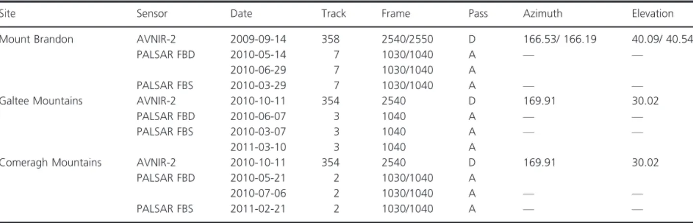
Table 1. Satellite data used for each of the study sites. Azimuth corresponds to the solar azimuth and elevation corresponds the sun elevation angle, both in degrees. D corresponds to acquisitions from a descending orbit and A corresponds to acquisitions from an ascending orbit.
Site Sensor Date Track Frame Pass Azimuth Elevation
Mount Brandon AVNIR-2 2009-09-14 358 2540/2550 D 166.53/ 166.19 40.09/ 40.54
PALSAR FBD 2010-05-14 7 1030/1040 A — —
2010-06-29 7 1030/1040 A
PALSAR FBS 2010-03-29 7 1030/1040 A — —
Galtee Mountains AVNIR-2 2010-10-11 354 2540 D 169.91 30.02
PALSAR FBD 2010-06-07 3 1040 A — —
PALSAR FBS 2010-03-07 3 1040 A — —
2011-03-10 3 1040 A
Comeragh Mountains AVNIR-2 2010-10-11 354 2540 D 169.91 30.02
PALSAR FBD 2010-05-21 2 1030/1040 A
2010-07-06 2 1030/1040 A — —
PALSAR FBS 2011-02-21 2 1030/1040 A — —
AVNIR-2, advanced visible and near infrared radiometer type 2; FBD, fine beam dual; FBS, fine beam single; PALSAR, phased array-type L-band synthetic aperture radar.
were calculated for all four bands (blue/green; blue/red;
blue/NIR; green/red; green/NIR; and red/NIR) and
included as input in the classifications. Although many of the VIs are highly correlated, the use of multiple VIs could offer a more complete characterization of the upland vegetation classes.
Texture measures
Eight texture measures (mean, homogeneity, contrast, variance, dissimilarity, entropy, correlation, and second moment) based on the grey-level co-occurrence matrix (GLCM) (Haralick et al. 1973) of the near infra-red band
and radar backscatter were created using a 3 93 kernel
size. These measures were included as they often provide unique information concerning the spatial pattern and variation in surface features and have been shown to improve classification accuracy (Lu and Weng 2007;
Paneque-Galvez et al. 2013).
Palsar
The FBS and FBD data were multi-looked by a factor of 2 in range and 4 in azimuth, and 1 in range and 4 in
azi-muth, respectively, to generate 15 915 m pixels. The
FBS and FBD scenes for each study area were co-regis-tered and speckle filco-regis-tered using a multi-temporal de Grandi filter (De Grandi et al. 1997), and subsequently radiometrically and geometrically calibrated and con-verted to dB using a range-doppler approach and a Next-Map 5 m spatial resolution DEM. The radar backscatter returned to the sensor is affected by the topography of the surface where certain terrain-induced distortions are present in areas with increased topographic relief. These areas were subsequently masked for each of the study
sites. For Mt Brandon, 15.08 km2 of the upland area out
of a total of 162 km2was masked (due to the presence of
cloud and/or shadow and terrain-induced distortions), corresponding to 9.3% of the total area. For the larger
scene (see Fig. 4), 62.29 km2was masked out of a total of
581.18 km2(land area only) which corresponds to 10.7%
of the total land surface area of the scene. 2.74 km2 of
the Comeraghs upland area of 103 km2and 13.38 km2 of
the total area of 943 km2 was masked, corresponding to
2.7% and 1.4% respectively. 2.27 km2 of the Galtees was
masked, corresponding to 2.7% and 0.4% of the upland
(83 km2) and total area (619 km2) respectively.
Ancillary variables
Two different groups of ancillary variables were chosen
for inclusion in the classifications: (1) Topographic–
ele-vation and slope, and (2) Soils. Soil and subsoil informa-tion was derived from the Teagasc-EPA Soils and Subsoils dataset (Fealy et al. 2009) and have a nominal working scale of 1:50,000 and elevation and slope data were obtained from a NextMap 5 m DEM. These parameters can influence the spatial distribution of upland vegetation species by affecting the amount of solar radiation and rainfall intercepted by the surface (Bennie et al. 2008, 2010), along with soil nutrient availability and moisture-holding capacity (Franklin 1995).
Classification schema and reference data
The broad-scale habitat classification scheme of Fossitt (2000) has been widely adopted by government authorities and the ecological community for habitat mapping in Ire-land. The classification schema adopted for the NPWS-funded National Survey of Upland Habitats (NSUH) is principally based on Fossitt (2000) and has been used in this study (see Table 3). A total of 15 classes (level 2) were identified and a stratified random sampling approach adopted for the selection of sample points. The three study sites have different class distributions and the proportion of each class varies relative to each site. Some classes are not present at some sites (e.g. lowland blanket bog) and some classes have a lower occurrence at other sites (e.g. exposed rock and montane heath at the Galtees). The sam-ple set reflects these differences and as much as possible, the class proportions of the sample data are representative of actual class proportions in the study area landscape. User interpretation of NSUH field survey data for Mount
Brandon (collected between May – Aug 2011), Galtee
Mountains (Aug –Sept 2011), Comeragh Mountains (Mar
– May 2010), Forest Inventory and Planning System
(FIPS) and MicrosoftBing Imagery aided the distinction
between the different classes.
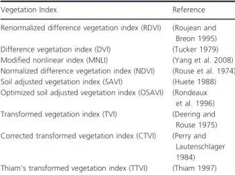
Table 2. Vegetation Indices selected for this study.
Vegetation Index Reference
Renormalized difference vegetation index (RDVI) (Roujean and Breon 1995)
Difference vegetation index (DVI) (Tucker 1979)
Modified nonlinear index (MNLI) (Yang et al. 2008)
Normalized difference vegetation index (NDVI) (Rouse et al. 1974) Soil adjusted vegetation index (SAVI) (Huete 1988) Optimized soil adjusted vegetation index (OSAVI) (Rondeaux
et al. 1996)
Transformed vegetation index (TVI) (Deering and
Rouse 1975) Corrected transformed vegetation index (CTVI) (Perry and
Lautenschlager 1984) Thiam‘s transformed vegetation index (TTVI) (Thiam 1997)
Classification
The Random Forests (RF) machine learning classifier (Breiman 2001) was used to relate the vegetation types to the satellite and ancillary data. RF was chosen as the pre-ferred classification method as it has consistently demon-strated its skill for vegetation mapping using various types of data (Cutler et al. 2007; Chapman et al. 2010; Bradter et al. 2011; Rodriguez-Galiano et al. 2012; Barrett et al. 2014; Feilhauer et al. 2014) and can handle high-dimensional datasets and not suffer from overfitting
(Bel-giu and Dragutß2016). RF builds an ensemble of
individ-ual decision-like trees from which a final prediction is made using a majority voting scheme. The individual trees are trained using a bootstrap sample of the training data (2/3 of samples) with the remaining 1/3 of samples used to test the classification and estimate the out-of-bag (OOB) error. In this study, RF models consisted of 200
trees. Separate models were generated to analyse the per-formance of the different data types separately and collec-tively. Eight different datasets were analysed to compare the change in classification accuracy depending on the selected input variables. These models concentrated on the use of optical only, radar only and various combina-tions of optical-derived and radar-derived variables along with certain ancillary variables. The influence of the dif-ferent input variables was calculated and the variable importances (based on the Gini importance) in the initial models were used to improve model fit and model parsi-mony. RF was implemented in Python 2.7.8 using the sci-kit learn library (Pedregosa et al. 2011).
Accuracy assessment
The results of all classifications were assessed using a stan-dard confusion matrix to calculate the overall accuracy
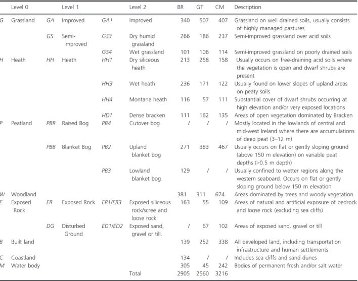
Table 3. Classification Schema and number of training samples. Class descriptions are adopted from Fossitt (2000).
Level 0 Level 1 Level 2 BR GT CM Description
G Grassland GA Improved GA1 Improved 340 507 407 Grassland on well drained soils, usually consists
of highly managed pastures
GS
Semi-improved
GS3 Dry humid
grassland
266 186 237 Semi-improved grassland over acid soils
GS4 Wet grassland 101 106 114 Semi-improved grassland on poorly drained soils
H Heath HH Heath HH1 Dry siliceous
heath
213 258 158 Usually occurs on free-draining acid soils where the vegetation is open and dwarf shrubs are present
HH3 Wet heath 236 171 122 Usually found on lower slopes of upland areas
on peaty soils
HH4 Montane heath 116 57 111 Substantial cover of dwarf shrubs occurring at high elevation and/or very exposed locations
HD1 Dense bracken 111 162 135 Areas of open vegetation dominated by Bracken
P Peatland PBR Raised Bog PB4 Cutover bog / / / Mostly located in the lowlands of central and
mid-west Ireland where there are accumulations of deep peat (3–12 m)
PBB Blanket Bog PB2 Upland
blanket bog
271 383 467 Usually occurs on flat or gently sloping ground (above 150 m elevation) on variable peat depths (>0.5 m depth)
PB3 Lowland
blanket bog
129 / / Usually confined to wetter regions along the western seaboard. Occurs on flat or gently sloping ground below 150 m elevation
W Woodland 381 311 674 Areas dominated by trees and woody vegetation
E Exposed
Rock
ER Exposed Rock ER1/ER3 Exposed siliceous rock/scree and loose rock
163 55 109 Areas of natural and artificial exposure of bedrock and loose rock (excluding sea cliffs)
DG Disturbed Ground
ED1/ED2 Exposed sand, gravel or till.
/ 67 102 Areas of exposed sand, gravel or till
B Built land 139 252 338 All developed land, including transportation
infrastructure and human settlements
C Coastland 134 / / Includes sea cliffs and sand dunes
M Water body 305 45 242 Bodies of permanent fresh and/or salt water
and the user‘s and producer‘s accuracies (Congalton 1991). An additional independent validation was also car-ried out for comparison to the RF OOB accuracies. A total of 876, 839, and 881 samples were randomly selected throughout the Mt Brandon, Galtee Mts, and Comeragh Mts study areas to create the independent accuracy assess-ment dataset. The statistical significance of the differences between the classification datasets was evaluated, using the Mc Nemar‘s test (Foody 2004), using the following formula:
z¼ f12ffiffiffiffiffiffiffiffiffiffiffiffiffiffiffiffiffiffif21 f12þf21
p ; (1)
wheref12indicates the number of samples correctly
classi-fied in the first classification, but incorrectly in the second
classification, and f21 represents the number of samples
correctly classified in the second classification, but incor-rectly classified in the first classification. The Mc Nemar‘s test has been commonly used in previous studies to eval-uate the variability between classifications (Duro et al. 2012; Belgiu et al. 2014). In this study, the significance
level ais set at 0.05 (zcritical value= 1.96).
Results
The accuracy assessments (overall accuracy, user’s and producer‘s accuracy) for the different classification data-sets are shown in Table 4. The overall accuracy (OA) values among the datasets vary from 59.8% to 94.3% across the three study locations. The highest overall
accu-racies (93.2–94.3%) were obtained for the combined
opti-cal, radar and ancillary data (viii), across all three study
areas. Most datasets achieved high accuracies (>~85%)
with the exception of the radar and texture measures
dataset (≤68%). The RF classifier displayed a relatively
consistent overall performance across the three study sites, however certain differences between classes were observed.
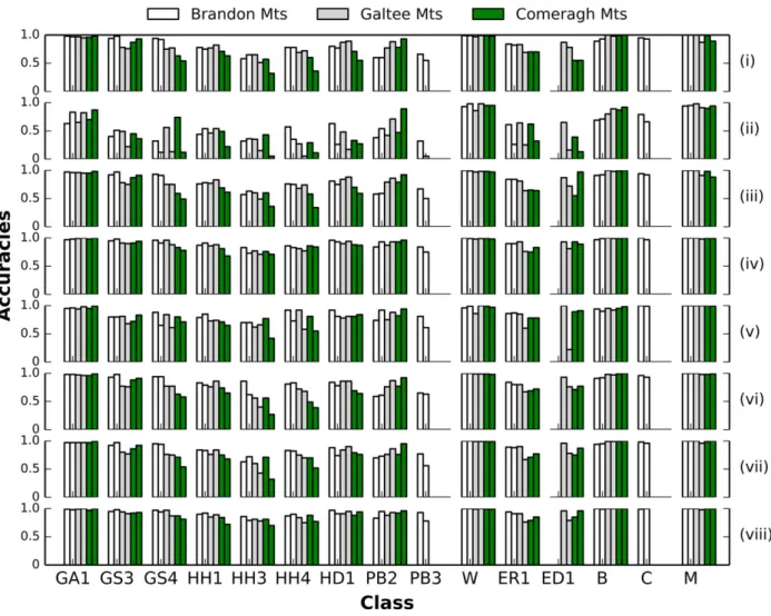
Figure 2 displays the producer‘s (PA) and user‘s (UA) accuracies for each of the eight classification datasets and provides more insight into the classification errors that are unique to specific classes. The producer‘s and user‘s accuracy represent the omission and commission errors respectively. The radar dataset (ii) displays the highest variation between PA and UA for many of the vegetation classes indicating that the radar and texture data tend to overestimate and when used alone, cannot reliably separate these classes. The lowest values for most datasets are confined to the heath classes, where differ-ences between the study areas become more readily apparent. When both optical and radar datasets are combined with the ancillary datasets (viii), these differ-ences between the study areas are less obvious.
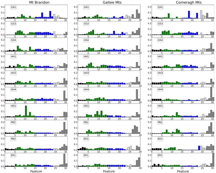
It can be seen that the increases in the accuracies achieved in some of the datasets by the addition of cer-tain variables are not large. RF produces a measure of the variable importance by analyzing the deterioration of the predictive ability of the model when each predictor vari-able is replaced in turn by random noise (Vincenzi et al. 2011). In general, the texture measures and radar data have low importance scores. The class-specific contribu-tions of different variables to the models are shown in Figure 3. Due to their negligible influence, the texture measures (optical and radar) have been omitted. In all three study areas, all models strongly relied on distinct spectral bands and band ratios. The influence of the ancil-lary data is variable between classes and study sites. The RF models were applied across the entire study areas to obtain vegetation cover for the whole regions (see Fig. 4), while the upland subsets in these study areas are shown in Figure 5. These maps were created using the (vii) data-set, without the inclusion of the soils and elevation
ancil-lary data. A 393 pixel majority filter was applied to the
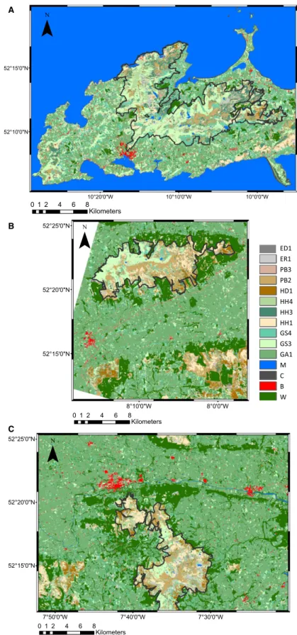
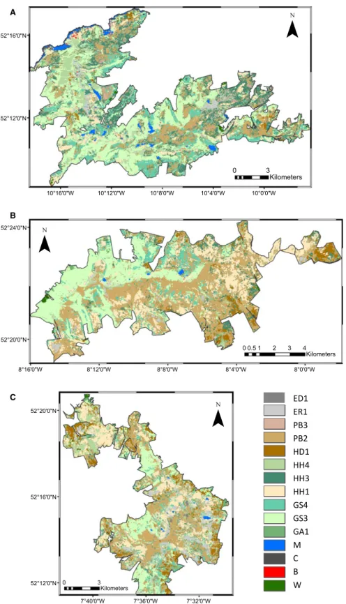
thematic outputs to improve the homogeneity of the final product. As can be seen from Figure 4, the dominant veg-etation cover in all areas is grasslands, and this is relatable to most areas in Ireland. There is very little forest cover on the Dingle Peninsula, while both the Galtee and Comeragh study areas have considerably larger forest areas, especially along the lower slopes of the upland areas. These areas usually represent lands that are mar-ginal for agriculture and since the 1950s, large extents have been afforested, supported through various govern-ment and EU incentive programmes. Concentrating on the upland subsets in Figure 5, the true value of upland areas in terms of habitat diversity is apparent. Mount Brandon (Fig. 5A) has extensive areas of wet heath, semi-improved (dry-humid acid) grasslands, blanket bog and dry siliceous heath. Large areas of montane heath are observed, especially along the western edge of the area making it quite distinctive when compared to the Galtee and Comeragh Mountains. From Figure 5(B), the domi-nant classes for the Galtee Mountains are dry-humid acid grassland along the north-west of the area, dry siliceous heath and blanket bog. Wet heath occurs less frequently, compared to the Mount Brandon area, though there are increased areas of wet grassland. Similar to the Galtees, the dominant classes in the Comeragh Mountains area (Fig. 5C) are blanket bog, dry siliceous heath and dry-humid acid grassland. Small areas of wet heath are scat-tered throughout the area and areas of dense bracken are prevalent along the eastern edges of the upland area.
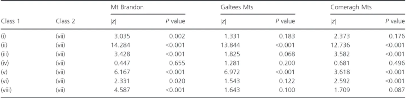
The results of the Mc Nemar’s test between classifica-tion (vii) and the others are displayed in Table 5 for all
study sites. McNemar0s test is non parametric and based
Table 4. Level 2 classification results. (i) O ptical and texture (ii) Radar and textu re (iii) Optical and texture and VIs (iv) Optical and ancillary data (v) Radar and ancillary data (vi) Op tical and Radar (vii) Opti cal an d Radar (inc texture and VIs) (viii) Optical and Rad ar and ancill ary data BR GT CM BR GT CM BR GT CM BR GT CM BR GT CM BR GT CM BR GT CM BR GT CM Overall Accuracy (%) 85.3 86.1 8 5.6 60 .0 59.8 68.0 84.6 85.5 84.9 93.0 92.4 93.1 87.4 83.2 88.7 85.6 85.8 8 6.2 88 .4 86.4 88.5 94.3 93.2 93.8 Improved grasslan d (GA1) PA 0.98 0.97 0.96 0 .63 0.65 0.70 0.97 0.96 0.95 0.97 0.99 0.98 0.95 0.94 0.95 0.98 0.97 0.96 0 .97 0.97 0.97 0.99 0.99 0.97 UA 0.97 0.95 0.98 0 .83 0.82 0.87 0.96 0.95 0.98 0.98 1.00 1.00 0.96 0.98 0.99 0.98 0.96 0.99 0 .97 0.97 0.99 0.98 1.00 1.00 Dry humid grassland (GS3 ) PA 0.94 0.78 0.87 0 .40 0.49 0.45 0.92 0.78 0.87 0.95 0.91 0.91 0.80 0.81 0.72 0.93 0.77 0.88 0 .92 0.80 0.86 0.95 0.94 0.92 UA 0.98 0.76 0.93 0 .51 0.22 0.36 0.97 0.75 0.91 0.98 0.90 0.94 0.80 0.68 0.83 0.98 0.76 0.91 0 .97 0.77 0.92 0.98 0.91 0.93 Wet grassland (GS4) PA 0.94 0.75 0.63 0 .32 0.56 0.74 0.93 0.75 0.59 0.96 0.96 0.83 0.88 0.84 0.80 0.94 0.77 0.63 0 .95 0.76 0.71 0.97 0.97 0.87 UA 0.92 0.77 0.54 0 .12 0.13 0.12 0.91 0.75 0.49 0.91 0.88 0.78 0.65 0.61 0.71 0.94 0.77 0.58 0 .94 0.75 0.54 0.94 0.87 0.81 Dry siliceous heath (HH1) PA 0.78 0.77 0.71 0 .44 0.46 0.49 0.76 0.77 0.69 0.87 0.86 0.81 0.79 0.73 0.71 0.83 0.76 0.74 0 .84 0.76 0.75 0.90 0.85 0.84 UA 0.75 0.82 0.63 0 .54 0.54 0.22 0.78 0.83 0.61 0.91 0.88 0.68 0.85 0.74 0.65 0.79 0.86 0.65 0 .83 0.84 0.68 0.92 0.89 0.72 Wet heath (HH3) PA 0.58 0.65 0.57 0 .32 0.35 0.43 0.57 0.60 0.60 0.83 0.77 0.76 0.70 0.62 0.77 0.56 0.56 0.56 0 .63 0.60 0.71 0.86 0.81 0.81 UA 0.65 0.51 0.32 0 .36 0.15 0.05 0.63 0.49 0.36 0.73 0.71 0.71 0.70 0.66 0.42 0.62 0.40 0.27 0 .72 0.43 0.32 0.79 0.78 0.70 Montane heath (HH4) PA 0.78 0.69 0.60 0 .57 0.27 0.29 0.76 0.68 0.58 0.86 0.81 0.86 0.92 0.92 0.81 0.81 0.72 0.49 0 .83 0.75 0.70 0.87 0.84 0.88 UA 0.78 0.72 0.36 0 .35 0.05 0.11 0.75 0.74 0.34 0.83 0.77 0.84 0.73 0.58 0.55 0.83 0.68 0.39 0 .82 0.70 0.52 0.90 0.75 0.77 Dense bracken (HD1) PA 0.80 0.87 0.71 0 .63 0.48 0.33 0.81 0.84 0.70 0.96 0.90 0.88 0.92 0.78 0.81 0.84 0.86 0.69 0 .88 0.84 0.79 0.97 0.91 0.88 UA 0.77 0.89 0.55 0 .26 0.17 0.27 0.75 0.88 0.59 0.93 0.94 0.87 0.81 0.81 0.84 0.78 0.86 0.64 0 .74 0.90 0.76 0.91 0.95 0.94 Upland blanket bo g (PB2) PA 0.60 0.77 0.78 0 .38 0.42 0.47 0.58 0.79 0.79 0.84 0.87 0.93 0.74 0.75 0.82 0.59 0.76 0.77 0 .70 0.76 0.76 0.83 0.88 0.92 UA 0.60 0.88 0.93 0 .54 0.71 0.89 0.59 0.86 0.92 0.93 0.93 0.96 0.92 0.88 0.94 0.61 0.87 0.92 0 .73 0.86 0.95 0.95 0.93 0.96 Lowland blanket bog (PB3) PA 0.66 / / 0 .32 / / 0.67 / / 0.84 / / 0.81 / / 0.65 / / 0 .77 / / 0.93 / / UA 0.55 / / 0 .05 / / 0.50 / / 0.75 / / 0.61 / / 0.53 / / 0 .56 / / 0.78 / / Woodland (W) PA 0.99 0.97 0.99 0 .93 0.86 0.95 1.00 0.97 0.98 1.00 0.98 0.99 0.96 0.86 0.99 1.00 0.99 0.99 1 .00 0.99 0.99 1.00 0.99 0.99 UA 0.99 0.99 0.98 0 .98 0.98 0.95 0.99 0.98 0.97 0.99 0.99 0.98 0.99 1.00 0.97 1.00 0.99 0.98 1 .00 0.99 0.99 1.00 1.00 0.99 Exposed Rock (ER1) PA 0.84 0.83 0.70 0 .61 0.64 0.62 0.84 0.81 0.65 0.90 0.93 0.75 0.86 0.85 0.78 0.84 0.80 0.69 0 .89 0.90 0.71 0.94 0.91 0.79 UA 0.82 0.69 0.68 0 .26 0.25 0.32 0.84 0.64 0.64 0.90 0.76 0.83 0.87 0.60 0.78 0.80 0.67 0.72 0 .88 0.67 0.77 0.91 0.76 0.85 Disturbed grou nd (ED1) PA / 0.87 0.55 / 0.65 0.39 / 0.87 0.55 / 0.93 0.93 / 1.00 0.89 / 0.93 0.71 / 0.96 0.75 / 0.96 0.85 UA / 0.78 0.97 / 0.16 0.13 / 0.72 0.97 / 0.81 0.89 / 0.22 0.91 / 0.76 0.77 / 0.78 0.87 / 0.79 0.96 Builtland (B) PA 0.89 1.00 0.99 0 .69 0.80 0.87 0.91 1.00 0.99 0.97 1.00 0.99 0.94 0.95 0.95 0.91 0.98 0.99 0 .94 0.99 0.99 1.00 1.00 1.00 UA 0.93 0.98 1.00 0 .71 0.89 0.92 0.92 0.98 1.00 0.99 0.99 1.00 0.90 0.92 0.98 0.92 0.97 1.00 0 .95 0.99 1.00 0.99 1.00 1.00 ( Continued )
hypothesis of no significant differences between
classifica-tions (e.g. (i)= (vii)). For all three sites, the difference
between (vii) and (ii) and (vii) and (v) were significantly
different (P<0.001). The difference between (vii) and
(iii) was significantly different (P<0.001) at both the Mt
Brandon and Comeragh Mts sites. Mt Brandon displayed
significant differences (P<0.05) between all
classifica-tions except (vii) and (iv) while the Comeragh Mts also
displayed significant differences (P<0.001) between (vii)
and (iii) and (vii) and (vi).
Discussion
The results from this study demonstrate the advantage of integrating EO satellite data from multiple sensors to improve vegetation mapping in upland regions. Even though it may not be surprising that the multispectral data outperforms the radar data, there is merit in incorporating both data types in the classifier models. One of the first published studies to investigate radar differences between upland and lowland vegetation was by Krohn et al. (1983) using L-band SEASAT data. Since then, few published studies on the use of radar for mapping uplands can be found in the literature. The results from this study reveal that a short time series of L-band radar data cannot exclu-sively separate all the distinct vegetation classes used in this analysis. The results show that combined optical and radar data obtain the highest classification accuracies, in agree-ment with previous studies (e.g. Bagan et al. (2012)). The inclusion of ancillary datasets containing information on the soil and elevation further improves the classification accuracies (between 5 and 27%, depending on the input classification dataset) and is similar to that found in previ-ous studies for both optical (Sesnie et al. 2008) and radar data (Barrett et al. 2014). When several vegetation classes are grouped into broader habitat types, classification accu-racies also show an improvement. There is little difference between level 0 and level 1 accuracies and in most cases, the lower level classifications show only a marginal improvement upon level 2 accuracies (see Fig. S1 and Tables S1, S2). To determine the stability of the level 2 clas-sification results, 25 iterations of the RF clasclas-sifications were run for the optical and radar dataset (vii) where the maxi-mum variation observed in OA for Mt Brandon was 1.01%, Galtee Mts was 0.71%, and Comeragh Mts was 0.69%.
Relative importance of explanatory variables
It can be seen from Figure 3 that the radar data has low importance scores for most of the vegetation classes, with the lowest scores obtained for the GS3 and PB2
Table 4. Continued. (i) Op tical and texture (ii) Radar and texture (iii) Optical and texture and VIs (iv) Optical and ancillary data (v) Radar and ancillary data (vi) Op tical and Radar (vii) Optical and R adar (inc texture and VIs) (viii) Optical and Rad ar and ancillary data BR G T CM BR GT CM BR GT CM BR GT CM BR GT CM BR G T CM BR GT CM BR GT CM Coastland (C) PA 0.95 / / 0.79 / / 0.94 / / 1.00 / / 1.00 / / 0.96 / / 0 .98 / / 0.99 / / UA 0.93 / / 0.66 / / 0.92 / / 0.97 / / 0.99 / / 0.93 / / 0 .96 / / 1.00 / / Water body (M) PA 1.00 1.00 0 .99 0.94 0.98 0.90 1.00 1.00 0.98 1.00 1.00 0.99 1.00 1.00 1.00 1.00 1.00 0.98 1 .00 1.00 0.99 1.00 1.00 1.00 UA 1.00 0.87 0 .89 0.95 0.91 0.94 1.00 0.91 0.88 1.00 0.98 0.99 1.00 1.00 0.99 1.00 0.98 0.99 1 .00 0.96 1.00 1.00 0.98 1.00 PA, producer accuracy; UA, user accuracy for the different datasets at each of the three study sites. BR, Mount Brandon; GT, Galtee Mountains; CM, Come ragh Mountains.
classes. This is likely due to the long wavelength of the
radar signal (k=23.6 cm) which penetrates through the
vegetation canopy and returns mostly information about the underlying soil properties. Shorter wavelength (e.g. C- or X-band) backscatter is influenced more by the vegetation canopy and may provide more information on the plant geometry that could facilitate the distinc-tion of different upland vegetadistinc-tion classes. Within the optical domain, the NIR signal is particularly useful for discriminating between grassland types (GA1, GS3 and GS4) while the green and red spectral bands perform well for distinguishing between the heath classes (HH1, HH3 and HH4) and blanket bog (PB2). The spectral band ratios (blue/red and green/red) performed espe-cially well in separating dense bracken (HD1), and in general performed better than the vegetation indices. The greater importance of these band ratios is likely due to the higher reflectance of bracken compared to other vegetation in autumn, especially in the red wavelengths
due to the higher amount of underlying dead litter. Similar findings were observed by Holland and Aplin (2013) for winter acquisitions.
Factors such as the bare soil, moisture conditions, solar zenith angle and the atmosphere can impact on the effective use of VIs for distinguishing vegetation types (Jackson and Huete 1991). Soil-adjusted indices such as SAVI and OSAVI minimise the soil background influence but do not outperform other VIs, indicating a likely negligible influence of bare soil on the classifica-tions. In fact, the nine VIs investigated in this study perform similarly across the different study areas. The exception is for the improved grassland (GA1) class where the DVI and renormalized difference vegetation index (RDVI) revealed the highest discriminatory power for the Mount Brandon and Comeragh Mountains. In both of these areas, the NIR channel also had a higher influence than other spectral bands or indices. This is likely due to the strong absorption of electromagnetic
Figure 2. Producers and User‘s accuracies, represented as the first and second column at each of the three study sites is displayed for the eight different classification datasets (i–viii) and correspond with those as presented in Table 4.
radiation in the red wavelengths (0.61–0.69lm) by chlorophyll in pastures and it‘s high reflectance in the NIR region. RDVI is similar to NDVI but tends to be more sensitive to changes in vegetation coverage under low leaf area index conditions.
Elevation is one of the most important factors deter-mining the broad-scale distribution of upland vegetation as it influences precipitation and temperature. Thus, ele-vation controls the ecological and physiological adapta-tions of various plant species (Lomolino 2001) and the significance of this variable and to a lesser extent, the slope can be seen across most of the classes. The high explanatory power of these variables is not surprising, as
upland grasslands and heaths tend to occur on sloping ground, and montane heaths generally occur at high ele-vations. Similarly, blanket bogs usually occur on level ground or gentle slopes. Furthermore, they generally occur on deep peaty soils and the results indicate that the soil and subsoil variables had a high importance in this class also. The particular importance of soil characteristics for vegetation mapping has been demonstrated in previ-ous studies by Rogan et al. (2003), Barrett et al. (2014), and Gartzia et al. (2014).
Studies within different scientific disciplines (e.g. bioin-formatics, statistics, ecology) suggest RF variable impor-tance measures can display a bias towards highly
Figure 3. Variable importance scores of the different classes for the three study areas. Apart from the mean, all texture measures were excluded as their importance was negligible. Radar backscatter data (black) represent the first four (Galtee Mountains) and five (Mount Brandon and Comeragh Mountains) variables followed by the four spectral bands (b1, b2, b3, b4) and spectral band ratios (b1b2, b1b3, b1b4, b2b3, b2b4, b3b4) in green. The vegetation indices (NDVI, SAVI, OSAVI, DVI, CTVI, TVI, TTVI, RDVI, and MNLI) are in blue with the band 4 mean, HH polarization mean, and HV polarization in light grey. The final four variables are the soil, subsoil, elevation, and slope (dark grey). NDVI, normalized difference vegetation index; OSAVI, optimized soil adjusted vegetation index; RDVI, renormalized difference vegetation index; SAVI, soil adjusted vegetation index.
10°0'0"W 10°10'0"W 10°20'0"W 52°15'0"N 52°10'0"N 012 4 6 8 Kilometers 7°30'0"W 7°40'0"W 7°50'0"W 52°25'0"N 52°20'0"N 52°15'0"N 012 4 6 8 Kilometers 8°0'0"W 8°10'0"W 52°25'0"N 52°20'0"N 52°15'0"N 012 4 6 8 Kilometers ED1 ER1 PB3 PB2 HD1 HH4 HH3 HH1 GS4 GS3 GA1 M C B W A B C
Figure 4. Maps derived from the optical and radar datasets (vii) for (A) Mount Brandon, (B) Galtee Mountains, and (C) Comeragh Mountain study areas. The delineated regions correspond to the upland areas of interest within each area.
8°0'0"W 8°4'0"W 8°8'0"W 8°12'0"W 8°16'0"W 52°24'0"N 52°20'0"N 00.51 2 3 4 Kilometers 7°32'0"W 7°36'0"W 7°40'0"W 52°20'0"N 52°16'0"N 52°12'0"N 0 3 Kilometers 10°0'0"W 10°4'0"W 10°8'0"W 10°12'0"W 10°16'0"W 52°16'0"N 52°12'0"N 0 3 Kilometers ED1 ER1 PB3 PB2 HD1 HH4 HH3 HH1 GS4 GS3 GA1 M C B W A B C
Figure 5. Maps of the upland areas of (A) Mount Brandon, (B) Galtee Mountains, and (C) Comeragh Mountain study areas. These areas correspond to the delineated regions in Figure 3.
correlated variables (Strobl et al. 2008; Genuer et al. 2010; Ellis et al. 2012). This bias can be lessened by increasing the subsample size of input variables at each node but at the expense of increasing the generalization error and decreasing the overall accuracy (Breiman 2001). Although not considered here, approaches such as the conditional permutation method (Strobl et al. 2008) could be explored as an alternative importance measure in future studies.
Predicted output map uncertainty
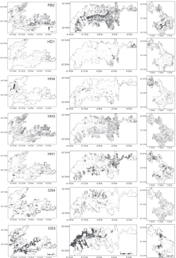
The retrieval of habitat information in upland areas using EO data is challenging due to the variable topography and the difficulty of obtaining cloud-free acquisitions in these regions. Furthermore, habitat delineation is more difficult to achieve as the landscape is more heteroge-neous (in terms of composition and structure) and con-sists of a number of interlinked habitats at different scales (spatial, temporal and spectral) (Varela et al. 2008). In this study, misclassification has occurred within and between subclasses of the main vegetation classes of inter-est (grassland, heaths, and blanket bog). An important feature of the RF algorithm is the ability to compute class probabilities in order to quantify the level of uncertainty in the predicted output maps. The probability of correct classification for each class was calculated to make this uncertainty explicitly available, whereby the relative pro-portion of each vegetation class per pixel is provided in Figure 6. The predicted probabilities of the main vegeta-tion classes are shown, where the darkest areas represent the pixels with the lowest uncertainty of the assigned class. The classes with the highest overall probabilities in each of the study sites are dry humid acid grasslands (GS3), blanket bogs (PB2), and dry siliceous heath (HH1). Ireland is the most important European country for blanket bog habitats and contains almost 8% of the worldwide blanket bog resource, thus these areas are of prime conservation value. Furthermore, these expanses represent a significant active natural carbon sink (Tomlin-son 2005; Bullock et al. 2012).
Comparison with additional independent validation dataset
Evaluation of classification accuracy, using the OOB accu-racies reported in the RF algorithm have generally been shown to be a reliable measure of classification accuracy (Lawrence et al. 2006; Devaney et al. 2015). Belgiu and
Dragutß(2016) suggest that this claim requires further
val-idation using a variety of datasets and application areas. In this study, an additional independent validation was performed and the results are presented in Table S3. In all cases, the accuracies obtained for the independent
vali-dation were, on average 5.12.5% lower than the
achieved OOB accuracies for all three study areas. The radar and ancillary dataset (v) had the largest differences, ranging between 8.4 and 11.6%, while the optical and radar (including texture measures and VIs) (vii) had the lowest, ranging between 2.5 and 3.3%. Although many studies have demonstrated the ability of RF to perform well on high dimensional data, Millard and Richardson (2015) found that RF can underestimate the error and recommend reducing the dimensionality of high dimen-sional datasets to significantly reduce the difference between OOB and independent assessment accuracies.
EO data acquisition timing and spatial resolution
The similarity of accuracies between the study areas may be attributable in part to the similar acquisition periods of the optical and radar data for each of the study areas. The AVNIR-2 scenes were acquired in September (Mount Brandon) and in October (Galtee and Comeragh Moun-tains) while the radar acquisitions were acquired between February and March and May and July for the FBS and FBD mode data respectively. The different modes of PAL-SAR data were only available for certain times of year, as part of JAXA‘s systematic observation strategy, whereby FBS mode acquisitions were available between January and April, and FBD mode acquisitions were available between May and October.
Table 5. Summary of the classification comparisons for the three study areas.
Mt Brandon Galtees Mts Comeragh Mts
Class 1 Class 2 |z| Pvalue |z| Pvalue |z| Pvalue
(i) (vii) 3.035 0.002 1.331 0.183 2.373 0.176 (ii) (vii) 14.284 <0.001 13.844 <0.001 12.736 <0.001 (iii) (vii) 3.428 <0.001 1.825 0.068 3.582 <0.001 (iv) (vii) 0.447 0.655 1.281 0.200 0.681 0.496 (v) (vii) 6.167 <0.001 6.972 <0.001 3.618 <0.001 (vi) (vii) 2.331 0.020 1.543 0.122 2.592 <0.001 (viii) (vii) 4.587 <0.001 1.643 0.100 1.709 0.087
10°0'W 10°4'W 10°8'W 10°12'W 10°16'W 52°16'N 52°12'N 0 3 Km GS3 10°0'W 10°4'W 10°8'W 10°12'W 10°16'W 52°16'N 52°12'N GS4 10°0'W 10°4'W 10°8'W 10°12'W 10°16'W 52°16'N 52°12'N HD1 10°0'W 10°4'W 10°8'W 10°12'W 10°16'W 52°16'N 52°12'N HH1 10°0'W 10°4'W 10°8'W 10°12'W 10°16'W 52°16'N 52°12'N HH3 10°0'W 10°4'W 10°8'W 10°12'W 10°16'W 52°16'N 52°12'N HH4 10°0'W 10°4'W 10°8'W 10°12'W 10°16'W 52°16'N 52°12'N PB2 High : 1 Low : 0 8°0'W 8°4'W 8°8'W 8°12'W 8°16'W 52°24'N 52°20'N 0 3 Km 8°0'W 8°4'W 8°8'W 8°12'W 8°16'W 52°24'N 52°20'N 8°0'W 8°4'W 8°8'W 8°12'W 8°16'W 52°24'N 52°20'N 8°0'W 8°4'W 8°8'W 8°12'W 8°16'W 52°24'N 52°20'N 8°0'W 8°4'W 8°8'W 8°12'W 8°16'W 52°24'N 52°20'N 8°0'W 8°4'W 8°8'W 8°12'W 8°16'W 52°24'N 52°20'N 8°0'W 8°4'W 8°8'W 8°12'W 8°16'W 52°24'N 52°20'N 7°32'W 7°36'W 7°40'W 52°20'N 52°16'N 52°12'N 0 3Km 7°32'W 7°36'W 7°40'W 52°20'N 52°16'N 52°12'N 7°32'W 7°36'W 7°40'W 52°20'N 52°16'N 52°12'N 7°32'W 7°36'W 7°40'W 52°20'N 52°16'N 52°12'N 7°32'W 7°36'W 7°40'W 52°20'N 52°16'N 52°12'N 7°32'W 7°36'W 7°40'W 52°20'N 52°16'N 52°12'N 7°32'W 7°36'W 7°40'W 52°20'N 52°16'N 52°12'N
Figure 6. Prediction probabilities for the main classes of interest for the upland areas of Mount Brandon (left), Galtee Mountains (middle) and Comeragh Mountains (right). Darker areas represent higher probabilities while the lighter areas indicate low probabilities. Class designations correspond to those in Table 3.
Vegetation has unique spectral signatures which evolve with the plant life cycle during the year. Characteristics such as pigmentation, water content and physiological structure affect the reflectance, absorption, and transmittance of plant leaves, stems and flowers. In this regard, the time of year of image acquisition will have a strong bearing on the classification accuracy and the ability to distinguish differ-ent types of vegetation. Nonetheless, it is difficult to iddiffer-entify an optimal temporal window for operational monitoring of all upland vegetation types (Cole et al. 2014), although acquisitions around September are considered optimum as most upland vegetation types are fully developed (Mills et al. 2006). The spectral similarity between different vege-tation types during the summer often limits the ability of acquisitions during these months to reliably distinguish between vegetation types. Ideally, a dense time series of data would allow this to be investigated further as the use of multitemporal data can account for the seasonal variation in vegetation and provide more accurate classifications (Gillanders et al. 2008). This could also open up the possi-bilities of monitoring grazing management (under- and over-grazing) more effectively and identify burning.
In addition to multitemporal data, a higher discrimina-tion between classes where misclassificadiscrimina-tions were high could be achieved with data from several spectral bands. For example, Feilhauer et al. (2014) successfully demon-strated the use of simulated multispectral data at 6 m, 10 m, 20 m and 60 m spatial resolution in providing detailed information on the distribution of habitat types. Similarly, Holland and Aplin (2013) found 4 m spatial res-olution IKONOS imagery not to be comprehensively supe-rior to Landsat (30 m spatial resolution) for mapping bracken at an uplands site in the UK. Similar findings were observed by Rocchini (2007) and Nagendra et al. (2010). All of these studies found spectral information to be much more important than spatial resolution. With the success-ful launch of medium spatial resolution sensors such as Sentinel-2 on 23rd June 2015 and future launch of the environmental mapping and analysis program (EnMAP) hyperspectral satellite (providing global coverage at 30 m spatial resolution in 232 spectral channels) in 2018, a valu-able and inexpensive source of information to derive spa-tially complete vegetation information for upland areas in a consistent and regular manner can be provided. More-over, the perceived inadequacy of medium spatial resolu-tion data may be overcome by incorporating informaresolu-tion on the class probabilities as a measure of quantifying the level of uncertainty in the predicted output maps.
Conclusion
In upland areas, meteorological, hydrological and ecologi-cal conditions often change substantially over relatively
short distances and thus contain a high diversity of habi-tats and species. Improving our knowledge on upland environments will give valuable insights into holistic envi-ronmental processes, aiding the development of sustain-able land management strategies for managing the effects of climate change, dormancy and promote conservation
of terrestrial and aquatic biodiversity (Nogues-Bravo et al.
2007; Ramchunder et al. 2009; Hodd et al. 2014). EO provides the only means of measuring the characteristics of habitats across broad areas and detecting environmen-tal changes that occur as a result of human or natural processes in these areas on a frequent basis (Kerr and Ostrovsky 2003; Turner et al. 2003; Duro et al. 2007; Nagendra et al. 2014). With the current availability of satellite EO data at low or no cost and an increased num-ber of satellites in orbit or planned, there has never been a better time to incorporate EO data into operational veg-etation mapping and monitoring programmes. EO data will never likely provide the fine-scale information that only field measurements can provide but can offer a pow-erful complimentary information source (Spanhove et al. 2012; Feilhauer et al. 2014; Pettorelli et al. 2014b; O’Con-nor et al. 2015). From this study, it can be concluded that
medium spatial resolution (~15 m) satellite data acquired
from optical and microwave sensors offers a basis for supporting mapping and monitoring of upland vegeta-tion. The mapping approach has been demonstrated over large areas in three distinctive upland regions, indicating the consistency and the transferability of the method.
Acknowledgements
This study was funded by the Environmental Protection Agency (EPA) under the Science, Technology, Research and Innovation for the Environment (STRIVE)
pro-gramme 2007–2013. The authors thank the National
Parks and Wildlife Service (NPWS) for providing the field survey data from the National Survey of Upland Habitats (NSUH) programme and also the European Space Agency (ESA) for providing the satellite data through Cat-1 pro-posal ID 28407. The authors are grateful to John Finn in Teagasc for his assistance throughout this study and would also like to thank the referees and the associate editor for their valuable comments which have helped improve the original manuscript.
Conflicts of Interest
The authors declare no conflicts of interest.
References
Bagan, H., T. Kinoshita, and Y. Yamagata. 2012. Combination of AVNIR-2, PALSAR, and polarimetric parameters for land
cover classification.IEEE Trans. Geosci. Remote Sens.50, 1318–1328.
Baghdadi, N., N. Boyer, P. Todoroff, M. El Hajj, and A. Begue. 2009. Potential of SAR sensors TerraSAR-X, ASAR/ ENVISAT and PALSAR/ALOS for monitoring sugarcane crops on Reunion Island.Remote Sens. Environ.113, 1724– 1738.
Barrett, B., I. Nitze, S. Green, and F. Cawkwell. 2014. Assessment of multi-temporal, multi-sensor radar and ancillary spatial data for grasslands monitoring in Ireland using machine learning approaches.Remote Sens. Environ. 152, 109–124.
Belgiu, M., and L. Dragutß. 2016. Random forest in remote sensing: a review of applications and future directions.
ISPRS J. Photogramm. Remote Sens.114, 24–31. Belgiu, M., L. Drǎgutß, and J. Strobl. 2014. Quantitative
evaluation of variations in rule-based classifications of land cover in urban neighbourhoods using WorldView-2 imagery.ISPRS J. Photogramm. Remote Sens.87, 205–215. Bennie, J., B. Huntley, A. Wiltshire, M. O. Hill, and R. Baxter.
2008. Slope, aspect and climate: spatially explicit and implicit models of topographic microclimate in chalk grassland.Ecol. Model.216, 47–59.
Bennie, J., A. Wiltshire, A. Joyce, D. Clark, A. Lloyd, J. Adamson, et al. 2010. Characterising inter-annual variation in the spatial pattern of thermal microclimate in a UK upland using a combined empirical–physical model.Agric. For. Meteorol.150, 12–19.
Bradter, U., T. J. Thom, J. D. Altringham, W. E. Kunin, and T. G. Benton. 2011. Prediction of National Vegetation Classification communities in the British uplands using environmental data at multiple spatial scales, aerial images and the classifier random forest.J. Appl. Ecol.48, 1057–1065. Breiman, L. 2001. Random forests.Mach. Learn45, 5–32. Buchanan, G., J. Pearce-Higgins, M. Grant, D. Robertson, and
T. Waterhouse. 2005. Characterization of moorland vegetation and the prediction of bird abundance using remote sensing.J. Biogeogr.32, 697–707.
Bullock, C. H., M. J. Collier, and F. Convery. 2012. Peatlands, their economic value and priorities for their future management–The example of Ireland.Land Use Policy29, 921–928.
Chan, J. C.-W., and D. Paelinckx. 2008. Evaluation of random forest and adaboost tree-based ensemble classification and spectral band selection for ecotope mapping using airborne hyperspectral imagery.Remote Sens. Environ.112, 2999–3011. Chan, J. C.-W., P. Beckers, T. Spanhove, and J. V. Borre. 2012.
An evaluation of ensemble classifiers for mapping Natura 2000 heathland in Belgium using spaceborne angular hyperspectral (CHRIS/Proba) imagery.Int. J. Appl. Earth Obs. Geoinf.18, 13–22.
Chapman, D. S., A. Bonn, W. E. Kunin, and S. J. Cornell. 2010. Random Forest characterization of upland vegetation
and management burning from aerial imagery.J. Biogeogr. 37, 37–46.
Cole, B., J. McMorrow, and M. Evans. 2014. Spectral monitoring of moorland plant phenology to identify a temporal window for hyperspectral remote sensing of peatland.ISPRS J. Photogramm. Remote Sens.90, 49–58. Congalton, R. G. 1991. A review of assessing the accuracy of
classifications of remotely sensed data.Remote Sens. Environ. 37, 35–46.
Corbane, C., S. Lang, K. Pipkins, S. Alleaume, M. Deshaves, V. Garcıa Millan, et al. 2015. Remote sensing for mapping natural habitats and their conservation status–New opportunities and challenges.Int. J. Appl. Earth Obs. Geoinf. 37, 7–16.
Council Directive 79/409/EEC. 1979. Council Directive 79/409/ EEC of 2 April 1979 on the conservation of wild birds. Council Directive 92/43/EEC. 1992. Council Directive 92/43/
EEC of 21 May 1992 on the conservation of natural habitats and of wild fauna and flora
Cutler, D. R., T. Edwards, K. Beard, A. Cutler, K. Hess, J. Gibson, et al. 2007. Random forests for classification in ecology.Ecology88, 2783–2792.
De Grandi, G., M. Leysen, J. Lee, and D. Schuler. 1997. Radar reflectivity estimation using multiple SAR scenes of the same target: technique and applications, Proceedings of the International Geoscience and Remote Sensing Symposium (IGARSS’97), Singapore, pp. 1047-1050.
Deering, D., and J. Rouse. 1975. Measuring ‘forage production’ of grazing units from Landsat MSS data, Proceedings of the 10th International Symposium on Remote Sensing of Environment, Ann Arbor, Mich, pp. 1169-1178.
Delalieux, S., B. Somers, B. Haest, T. Spanhove, J. Vanden Borre, and C. A. M€ucher, et al. 2012. Heathland conservation status mapping through integration of hyperspectral mixture analysis and decision tree classifiers.
Remote Sens. Environ.126, 222–231.
Devaney, J., B. Barrett, F. Barrett, J. Redmond, and O. John. 2015. Forest cover estimation in Ireland using radar remote sensing: a comparative analysis of forest cover assessment methodologies.PLoS ONE10, e0133583.
Duro, D. C., N. C. Coops, M. A. Wulder, and T. Han. 2007. Development of a large area biodiversity monitoring system driven by remote sensing. Prog. Phys. Geogr. 31, 235–260.
Duro, D. C., S. E. Franklin, and M. G. Dube. 2012. A comparison of pixel-based and object-based image analysis with selected machine learning algorithms for the
classification of agricultural landscapes using SPOT-5 HRG imagery.Remote Sens. Environ.118, 259–272.
Ellis, N., S. J. Smith, and C. R. Pitcher. 2012. Gradient forests: calculating importance gradients on physical predictors.
Evans, T. L., and M. Costa. 2013. Landcover classification of the Lower Nhecol^andia subregion of the Brazilian Pantanal Wetlands using ALOS/PALSAR, RADARSAT-2 and ENVISAT/ASAR imagery.Remote Sens. Environ.128, 118–137.
Fealy, R., S. Green, R. Meehan, T. Radford, C. Cronin, and M. Bulfin. 2009.Teagasc EPA Soil and Subsoils Mapping Project-Final Report. Teagasc 1 1-126 23123 R1. Teagasc, Dublin. Feilhauer, H., C. Dahlke, D. Doktor, A. Lausch, S.
Schmidtlein, G. Schulz, et al. 2014. Mapping the local variability of Natura 2000 habitats with remote sensing.
Appl. Veg. Sci.17, 765–779.
Foody, G. M. 2004. Thematic map comparison.Photogramm. Eng. Remote Sensing70, 627–633.
Fossitt, J. A. 2000.A guide to habitats in Ireland. The Heritage Council, Dublin.
Franklin, J. 1995. Predictive vegetation mapping: geographic modelling of biospatial patterns in relation to environmental gradients.Prog. Phys. Geogr.19, 474–499.
Gartzia, M., C. L. Alados, and F. Perez-Cabello. 2014. Assessment of the effects of biophysical and anthropogenic factors on woody plant encroachment in dense and sparse mountain grasslands based on remote sensing data.Prog. Phys. Geogr.38, 201–217.
Genuer, R., J.-M. Poggi, and C. Tuleau-Malot. 2010. Variable selection using random forests.Pattern Recogn. Lett.31, 2225–2236.
Gillanders, S. N., N. C. Coops, M. A. Wulder, S. E. Gergel, and T. Nelson. 2008. Multitemporal remote sensing of landscape dynamics and pattern change: describing natural and anthropogenic trends.Prog. Phys. Geogr.32, 503–528. Gillespie, T. W., G. M. Foody, D. Rocchini, A. P. Giorgi, and
S. Saatchi. 2008. Measuring and modelling biodiversity from space.Prog. Phys. Geogr.32, 203–221.
GRASS Development Team. 2012. Geographic Resources Analysis Support System (GRASS) Software, Open Source Geospatial Foundation Project. Avaliable at http://grass.osgeo.org. (accessed 21 October 2016)
Haralick, R. M., K. Shanmugam, and I. H. Dinstein. 1973. Pp. 610–621Textural features for image classification. IEEE Transactions on Systems, Man and Cybernetics. Hodd, R. L., D. Bourke, and M. S. Skeffington. 2014.
Projected range contractions of European protected oceanic montane plant communities: focus on climate change impacts is essential for their future conservation.PLoS ONE 9, e95147.
Holland, J., and P. Aplin. 2013. Super-resolution image analysis as a means of monitoring bracken (Pteridium aquilinum) distributions.ISPRS J. Photogramm. Remote Sens.75, 48–63. Huete, A. R. 1988. A soil-adjusted vegetation index (SAVI).
Remote Sens. Environ.25, 295–309.
Intermap Technologies. 2008. Comprehensive 3D Data for More Effective Analysis. Available at: http://
www.intermap.com/data/nextmap (accessed 4 April 2016).
Jackson, R. D., and A. R. Huete. 1991. Interpreting vegetation indices.Prev. Vet. Med.11, 185–200.
Kerr, J. T., and M. Ostrovsky. 2003. From space to species: ecological applications for remote sensing.Trends Ecol. Evol. 18, 299–305.
Krohn, M. D., N. Milton, and D. B. Segal. 1983. Seasat synthetic aperture radar (SAR) response to lowland vegetation types in eastern Maryland and Virginia.J. Geophy. Res. Oceans (1978–2012)88(C3), 1937–1952. Lausch, A., A. Schmidt, and L. Tischendorf. 2015. Data mining
and linked open data–New perspectives for data analysis in environmental research.Ecol. Model.295, 5–17.
Lawrence, R. L., S. D. Wood, and R. L. Sheley. 2006. Mapping invasive plants using hyperspectral imagery and Breiman Cutler classifications (RandomForest).Remote Sens. Environ. 100, 356–362.
Lees, B. G., and K. Ritman. 1991. Decision-tree and rule-induction approach to integration of remotely sensed and GIS data in mapping vegetation in disturbed or hilly environments.Environ. Manage.15, 823–831. Lomolino, M. 2001. Elevation gradients of species-density:
historical and prospective views.Glob. Ecol. Biogeogr.10, 3–13. Lu, D., and Q. Weng. 2007. A survey of image classification
methods and techniques for improving classification performance.Int. J. Remote Sens.28, 823–870. Lucas, R., A. Rowlands, A. Brown, S. Keyworth, and P.
Bunting. 2007. Rule-based classification of multi-temporal satellite imagery for habitat and agricultural land cover mapping.ISPRS J. Photogramm. Remote Sens.62, 165–185.
Lucas, R., K. Medcalf, A. Brown, P. Bunting, J. Breyer, D. Clewley, et al. 2011. Updating the Phase 1 habitat map of Wales, UK, using satellite sensor data.ISPRS J. Photogramm. Remote Sens.66, 81–102.
Lucas, R., P. Blonda, P. Bunting, G. Jones, J. Inglada, M. Arias et al. 2015. The Earth observation data for habitat
monitoring (EODHaM) system.Int. J. Appl. Earth Obs. Geoinf.37, 17–28.
MacDonald, D., J. Crabtree, G. Wiesinger, T. Dax, N. Stamou, P. Fleury, et al. 2000. Agricultural abandonment in mountain areas of Europe: environmental consequences and policy response.J. Environ. Manage.59, 47–69.
Mehner, H., M. Cutler, D. Fairbairn, and G. Thompson. 2004. Remote sensing of upland vegetation: the potential of high spatial resolution satellite sensors.Glob. Ecol. Biogeogr.13, 359–369.
Millard, K., and M. Richardson. 2015. On the importance of training data sample selection in random forest image classification: a case study in peatland ecosystem mapping.
Remote Sens.7, 8489–8515.
Mills, H., M. Cutler, and D. Fairbairn. 2006. Artificial neural networks for mapping regional-scale upland vegetation from high spatial resolution imagery.Int. J. Remote Sens.27, 2177– 2195.
Nagendra, H., D. Rocchini, R. Ghate, B. Sharma, and S. Pareeth. 2010. Assessing plant diversity in a dry tropical forest: comparing the utility of Landsat and IKONOS satellite images.Remote Sens.2, 478–496.
Nagendra, H., R. Lucas, R. J. Pradinho Honrado, R. Jongman, C. Tarantino, M. Adamo, et al. 2013. Remote sensing for conservation monitoring: assessing protected areas, habitat extent, habitat condition, species diversity, and threats.Ecol. Ind.33, 45–59.
Nagendra, H., P. Mairota, C. Marangi, R. Lucas, P. Dimopoulos, J. Pradinho Honrado, et al. 2014. Satellite earth observation data to identify anthropogenic pressures in selected protected areas.Int. J. Appl. Earth Obs. Geoinf. 37, 124–132.
Nogues-Bravo, D., M. B. Araujo, M. Errea, and J. Martinez-Rica. 2007. Exposure of global mountain systems to climate warming during the 21st Century.Glob. Environ. Change17, 420–428. O’Connor, B., C. Secades, J. Penner, R. Sonnenschein, A.
Skidmore, N. D. Burgess, et al. 2015. Earth observation as a tool for tracking progress towards the Aichi Biodiversity Targets.Remote Sens. Ecol. Conserv.1, 19–28.
Paneque-Galvez, J., J.-F. Mas, G. More, J. Cristobal, M. Orta-Martınez, A. Luz et al. 2013. Enhanced land use/cover classification of heterogeneous tropical landscapes using support vector machines and textural homogeneity.Int. J. Appl. Earth Obs. Geoinf.23, 372–383.
Pedregosa, F., G. Varoquanx, A. Gramfort, V. Michel, B. Thirion, O. Grisel, et al. 2011. Scikit-learn: Machine learning in Python.J. Machine Learn. Res.12, 2825–2830. Perrin, P. M., B. O’Hanrahan, J. R. Roche, and S. J. Barron.
2009.Scoping study and pilot survey for a National Survey and Conservation Assessment of Upland Vegetation and Habitats in Ireland. Unpublished report to National Parks & Wildlife Service, Department of Environment, Heritage and Local Government, Dublin.
Perry, C. R., and L. F. Lautenschlager. 1984. Functional equivalence of spectral vegetation indices.Remote Sens. Environ.14, 169–182.
Pettorelli, N., W. F. Laurance, T. G. O’Brien, M. Wegmann, H. Nagendra, and W. Turner. 2014a. Satellite remote sensing for applied ecologists: opportunities and challenges.
J. Appl. Ecol.51, 839–848.
Pettorelli, N., K. Safi, and W. Turner. 2014b. Satellite remote sensing, biodiversity research and conservation of the future.
Philos. Trans. R. Soc. B Biol. Sci.369, 20130190. Ramchunder, S., L. Brown, and J. Holden. 2009.
Environmental effects of drainage, drain-blocking and prescribed vegetation burning in UK upland peatlands.Prog. Phys. Geogr.33, 49–79.
Reed, M., A. Bonn, W. Slee, N. Beharry-Borg, J. Birch, I. Brown, et al. 2009. The future of the uplands.Land Use Policy26, S204–S216.
Rhodes, C. J., P. Henrys, G. M. Siriwardena, M. J.
Whittingham, and L. R. Norton. 2015. The relative value of
field survey and remote-sensing for biodiversity assessment.
Methods Ecol. Evol.6, 772–781.
Richter, R., and D. Schlapfer. 2011. Atmospheric/topographic correction for satellite imagery.DLR-German Aerospace Center: Wessling, Germany2011, 202.
Rocchini, D. 2007. Effects of spatial and spectral resolution in estimating ecosystema-diversity by satellite imagery.Remote Sens. Environ.111, 423–434.
Rodriguez-Galiano, V. F., B. Ghimire, J. Rogan, M. Chica-Olmo, and J. P. Rigol-Sanchez. 2012. An assessment of the
effectiveness of a random forest classifier for land-cover classification.ISPRS J. Photogramm. Remote Sens.67, 93–104. Rogan, J., J. Miller, D. Stow, J. Franklin, L. Levien, and C.
Fischer. 2003. Land-cover change monitoring with classification trees using Landsat TM and ancillary data.
Photogramm. Eng. Remote Sensing69, 793–804.
Rondeaux, G., M. Steven, and F. Baret. 1996. Optimization of soil-adjusted vegetation indices.Remote Sens. Environ.55, 95–107. Roujean, J.-L., and F.-M. Breon. 1995. Estimating PAR
absorbed by vegetation from bidirectional reflectance measurements.Remote Sens. Environ.51, 375–384.
Rouse, J.W., R. H. Haas, J. A. Schell, D. W. Deering, and J. C. Harlan. 1974. Monitoring the vernal advancement
retrogradation of natural vegetation. NASA/GSFC (Type III, Final Report), Greenbelt, MD.
Sarker, L. R., and J. E. Nichol. 2011. Improved forest biomass estimates using ALOS AVNIR-2 texture indices.Remote Sens. Environ.115, 968–977.
Sesnie, S. E., P. E. Gessler, B. Finegan, and S. Thessler. 2008. Integrating Landsat TM and SRTM-DEM derived variables with decision trees for habitat classification and change detection in complex neotropical environments.Remote Sens. Environ.112, 2145–2159.
Spanhove, T., J. Vanden Borre, S. Delalieux, B. Haest, and D. Paelinckx. 2012. Can remote sensing estimate fine-scale quality indicators of natural habitats?Ecol. Ind.18, 403–412. Strobl, C., A.-L. Boulesteix, T. Kneib, T. Augustin, and A.
Zeileis. 2008. Conditional variable importance for random forests.BMC Bioinformatics9, 1.
Teillet, P. M., B. Guindon, and D. G. Goodenough. 1982. On the slope-aspect correction of multispectral scanner data.
Can. J. Remote Sen.8, 84–106.
Thiam, A. K. 1997. Geographic Information System and Remote Sensing Methods for Assessing and Monitoring Land Degradation in the Shale: The Case of Southern Mauritania, Darks University.
Tomlinson, R. W. 2005. Soil carbon stocks and changes in the Republic of Ireland.J. Environ. Manage.76, 77–93. Tucker, C. J. 1979. Red and photographic infrared linear
combinations for monitoring vegetation.Remote Sens. Environ.8, 127–150.
Turner, W., S. Spector, N. Gardiner, M. Fladeland, E. Sterling, and M. Steininger. 2003. Remote sensing for biodiversity science and conservation.Trends Ecol. Evol.18, 306–314.
Vanden Borre, J., D. Paelinckxa, C. A. Mucherb, L. Kooistrac,€ B. Haestd, G. De Blusta, et al. 2011. Integrating remote sensing in Natura 2000 habitat monitoring: Prospects on the way forward.J. Nat. Conserv.19, 116–125.
Varela, R. D., P. R. Rego, S. C. Iglesias, and C. M. Sobrino. 2008. Automatic habitat classification methods based on satellite images: A practical assessment in the NW Iberia coastal mountains.Environ. Monit. Assess.144,
229–250.
Vincenzi, S., M. Zucchetta, P. Franzoi, M. Pellizzato, F. Pranovi, G. A. De Leo, et al. 2011. Application of a random forest algorithm to predict spatial distribution of the potential yield of Ruditapes philippinarum in the Venice lagoon, Italy.Ecol. Model.222, 1471–1478.
Waske, B., and M. Braun. 2009. Classifier ensembles for land cover mapping using multitemporal SAR imagery.ISPRS J. Photogramm. Remote Sens.64, 450–457.
Yang, Z., P. Willis, and R. Mueller. 2008. Impact of band-ratio enhanced AWIFS image to crop classification accuracy. Proceedings of Pecora 17, Available at: http://www. asprs. org/a/publications/proceedings/pecora17/0041. pdf.
Supporting Information
Additional supporting information may be found online in the supporting information tab for this article.
Figure S1. Overall accuracies for the classification datasets at level 0, level 1, and level 2 for (A) Mount Brandon, (B) Galtee Mountains, and (C) Comeragh Mountains.
The classification datasets (i–viii) correspond to those as
presented in Table 4.
Table S1. Level 1 classification results for the different data-sets at each of the three study sites. BR, Mount Brandon; GT, Galtee Mountains; and CM, Comeragh Mountains.
Table S2.Level 0 classification results for the different data-sets at each of the three study sites. BR, Mount Brandon; GT, Galtee Mountains; CM, Comeragh Mountains.
Table S3.Level 2 classification results (PA, producer accu-racy; UA, user accuracy) for the different datasets at each of the three study sites for the independent validation. BR, Mount Brandon; GT, Galtee Mountains; CM, Comeragh Mountains.