Quality Driven Wireless Sensor Network

(1)

QUALITY DRIVEN

WIRELESS SENSOR NETWORK

(2)

i

QUALITY DRIVEN WIRELESS SENSOR NETWORK

Thesis submitted to

National Institute of Technology, Rourkela for the award of the degree

of

Bachelor of Technology by

Harshit Ranjan

Under the guidance of

Prof. S. K. Das

Department of Electronics

&

Communication Engineering

National Institute of Technology, Rourkela

May, 2015

(3)

ii

Dept. of Electronics

&

Communication Engineering

National Institute of Technology Rourkela

Rourkela-769 008, Odisha, India. www.nitrkl.ac.in

May 10, 2015

Certificate

This is to certify that the thesis entitled, Quality Driven Wireless Sensor Network, submitted by Harshit Ranjan to National Institute of Technology Rourkela, is a record of bonafide research work carried under my supervision and is worthy of consideration for the award of the degree of Bachelor of Technology of the Institute.

Prof. S. K. Das Assistant Professor

Department of Electronics and Communication

Engineering

Place: NIT, Rourkela National Institute of Technology, Rourkela Date: 10th May, 2015 India 769 008

(4)

iii

Acknowledgements

I owe my gratitude to all the people who have contributed and helped in the completion of the thesis. First of all, I would thank my guide Prof. S. K. Das sir who inspired and helped me to work on Wireless Sensor Network. It is through his excellent knowledge of the topic and motivation throughout the year that I was able to complete my project as well as thesis. I am thankful to him for providing me the necessary resources and showing me the right direction to work. I am grateful to him for his kind support.

Further, I am thankful to all the professors of Electronics and Communication Department, especially Prof. K. K. Mahapatra for providing a platform and creating opportunity for the B.Tech students to work on a project to provide them in depth knowledge of the topic of their choice.

I am thankful to my friends who at times of need provided me with valuable suggestions and resources.

Finally, I thank my parents who supported me for the whole period of time and even more.

(5)

iv

Abbreviations

ACQUIRE Active Query Forwarding In Sensor Networks

APTEEN Adaptive Periodic Threshold-sensitive Energy Efficient sensor Network protocol

BS Base Station

CADR Constrained Anisotropic Diffusion Routing CDMA Code Division Multiple Access

CH Cluster Head

CSMA Carrier Sense Multiple Access

DC Data Centric

EAR Energy Aware Routing GAF Geographic Adaptive Fidelity GBR Gradient-Based Routing

GEAR Geographic and Energy Aware Routing GEDIR Geographic Distance Routing

GOAFR Greedy Other Adaptive Face Routing GPS Global Positioning System

HPAR Hierarchical Power Aware Routing IDSQ Information Driven Sensor Querying

IEEE Institute of Electrical and Electronics Engineers ILP Integer Linear Program

LEACH Low Energy Adaptive Clustering Hierarchy LML Local Markov Loops

MAC Medium Access Control

MCFA Minimum Cost Forwarding Algorithm MECN Minimum Energy Communication Network MFR Most Forward within Radius

PEGASIS Power Efficient Gathering in Sensor Information Systems QoS Quality of Service

SAR Sensor Aggregates Routing: SOP Self Organizing Protocol

(6)

v

SPIN Sensor Protocols for Information via Negotiation TDMA Time Division Multiple Access

TTDD Two-Tier Data Dissemination

TEEN Threshold-sensitive Energy Efficient sensor Network VGA Virtual Grid Architecture

(7)

vi

List of Figures

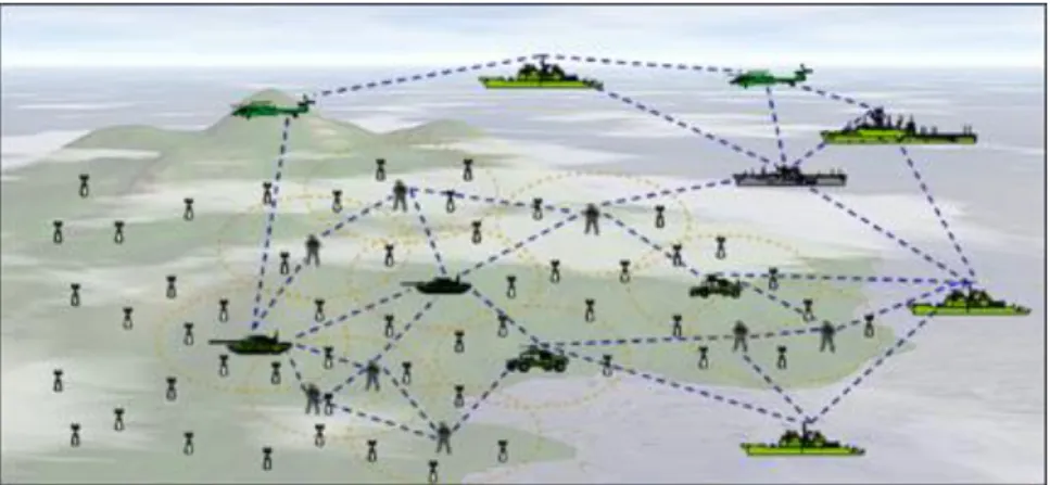
1.1: Example of WSN in Defense Application………..03

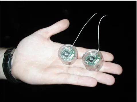
2.1: An actual sensor node……….06

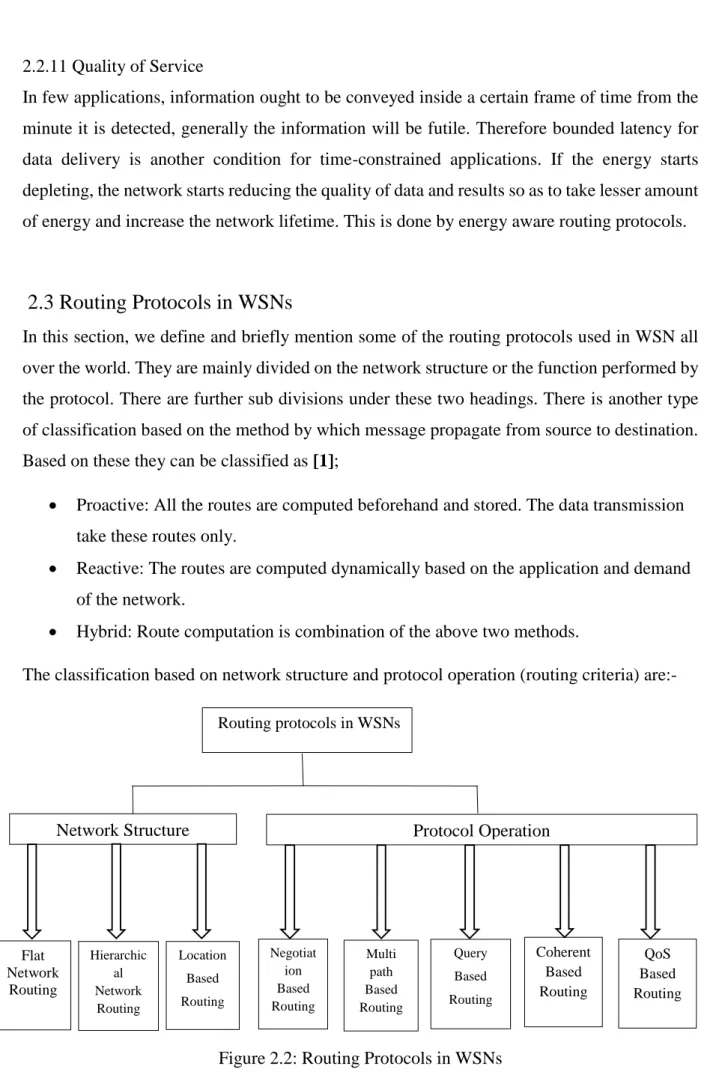
2.2: Routing Protocols in WSNs………10

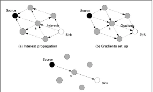
2.3: GBR from source to sink……….13

2.4: Application of COUGAR in an internet network………14

2.5: Difference between simple Flat and Hierarchical Routing………..15

2.6: Cluster based routing in LEACH………...15

2.7: Time line for operation of TEEN and APTEEN………...16

2.8: VGA in defense………17

2.9: Block diagram of a GAF Location based Routing………...18

2.10: Example of Multipath based Routing……….20

2.11: Query based Routing with node weights………21

3.1: Flowchart of WSN simulation………..26

3.2: Flowchart of WSN parameter calculation……….29

4.1: WSN Simulation for number of nodes = 50 and 4.1.1: Degree of nodes = 8………...34

4.1.2: Degree of nodes = 26……….34

4.2.2: Degree of nodes = 26………...35

4.3.2: Degree of nodes = 26……….36

4.4: Dynamic graph showing last highlighted node……….41

(8)

vii

Abstract

Wireless Sensor Network is a network consisting of numerous nodes that wirelessly transmit data packets through various routing protocols that it has been based on. In this paper, the networks and its classification has been explained. Various routing algorithms based on time, location of nodes, distribution of energy between them, etc. have been touched upon. There is a short description and final comparison between the various types of protocols so as to help in deciding which type of routing method should be used in a given network based on the requirements. Following the classification and comparison, there is a simulation for a wireless sensor network for various number and degree of nodes (to show compactness between nodes). Then analysis of various parameters like the shortest path, distance traversed by the path including all the mid-nodes, distance in units, number of messages traversed in one round of simulation, etc. are done using MATLAB. Due to their versatility, ease and efficiency in operation the wireless sensor networks find an extensive use in the modern world. Some of the common areas of their uses are process management, health care monitoring, area management, defense application, air pollution monitoring, forest fire detection, landslide detection, water quality monitoring, chemical agent detection, natural disaster prevention, data logging, etc. This diverse field of application makes the study and analysis of wireless sensor network one of the hottest topic in today’s world.

In short, this thesis introduces one to various wireless routing methods and concentrates on one of the most important parameter for quality improvement i.e. path; which indirectly improvises the time.

Keywords: Wireless Sensor Network, Nodes, Quality of Service, Transmission data rate, End-to-end delay, Data gathering, Link, Routing.

(9)

viii

Introduction

Preface

Wireless Sensor Network is a network of spatially distributed sensors (better known as nodes) that wirelessly monitors and controls various physical or environmental conditions [5]. In this section, we introduce you to WSN and some of the major factors based on which it is classified.

(12)

2

1.1

Introduction

Due to the advancement in technology and the growing demand of wireless communication systems, wireless sensor have become technically and economically more feasible. It comprises of a group of sensor nodes scattered over an area. The basic function of a node comprises sensing, processing, transmission, mobilizer, position finding system, and power units. It senses the change in physical and environmental conditions and transmits it wirelessly to the BS. The base station sends it to the required user or control office so that necessary steps can be taken. The selection of the correct WSN depends on a number of metrics like lifetime, coverage, cost, etc. For example, in defense application we use the network that is spread over a large area, having very fast response time, robust and having a high fault tolerance. There are lots of routing challenges and design issues which should be tackled to ensure a smooth functioning of the network. But everything is finally converging to the path and time taken by the data to reach the BS. If a given message takes less number of nodes to pass through and reach the base node then there will be lesser pressure on nodes that are not used. This will make each node to be used less frequently, hence increasing their lifetime. Therefore, the main objective of the thesis is to concentrate to find the shortest paths between any given pair of nodes. This factor will also help us in taking care of QoS. The simulation results show the networks ranging from 50 nodes to 400 nodes. More number of nodes ensure sensing of a larger area. Finding shortest paths between every two nodes and then analyzing it for distance, whether or not it will satisfy the energy and QoS requirement, messages processed per round of data gathering, highlighting the path taken by the message to travel from source node to the tail node and finding out which message will be feasible for usage. The model can also be used to determine the BS. The paths from one node to all others can be found and it can be done for each and every node. Finally comparing the total number of nodes that can be accessed by a given node, we can find the number of nodes that satisfy the QoS. Hence, the node with most number of other nodes sending messages on time (satisfying QoS) will be the Base Station. In this way it can help in a lots of situations of modern application of wireless sensor networks like defense application, industrial maintenance, health care, environment monitoring, etc.

(13)

3

Fig 1.1: Example of WSN in Defense Application

1.2 Motivation behind the Research Work

The increasing popularity of WSN have led to vast research and development in this area. There are many requirements from the user side like time limit, minimal signal interference, minimal blocking probability, more energy efficiency, higher lifetime and everything at as cheap cost as possible. Beside their presence everywhere would raise anyone’s curiosity to know and work on them. Hence, the thesis starts with a simple definition, classification, simulation of a WSN and ends on analyzing the results and satisfying certain factors by taking an example.

1.3 Problem Definition

Given the condition from user like;

 Number of nodes in the network

 Degree of the nodes

 Grid or random topology

We have to simulate a WSN and analyze the following:-

 Selection of a base node.

 Finding the shortest path of each node from the BS in terms of nodes involved in the path.

 Finding the distance between nodes.

 Highlighting the nodes involved in another dynamic graph.

 Finding the number of messages processed by each node in one round of data gathering.

(14)

4

1.4 Scope of the Thesis

The thesis simulates a proper WSN and finds out the shortest distances between nodes. It can be used in future works in the following areas:-

 Other analysis and calculations can be performed on the simulated model of WSN

 Floyd Warshall algorithm has been used to find out the shortest path. Dijkstra’s or few other methods can be implemented and results be compared for finding out the distances.

 QoS requirement can be adjusted and filled with the help of second program.

 The highlighting of shortest paths can be used in agriculture and defense application.

1.5 Organization of the Thesis

Following this introduction, the remaining part of the thesis is organized into following chapters:

Chapter 2: This chapter explains the theory and literature survey that has been done for the thesis. It includes the classification of various routing protocols, challenges and design issues in routing and brief theory on applications of WSN in various fields.

Chapter 3: This chapter describes the system model along with the MATLAB codes to implement the idea into a simulation.

Chapter 4: This chapter deals with the algorithm and flowchart of the model. Chapter 5: This chapter shows the simulation and analytical results.

Chapter 6: Finally, this chapter presents conclusion and discussion on application and limitations.

(15)

5

C H A P T E R

2

Literature Survey

Preface

This chapter presents the literature survey along with the classification and related discussions on the concept of WSN and Routing Protocols. It also discusses the challenges faced in routing and presents a comparison between various routing methods.

(16)

6

2.1 Introduction to Routing

Routing is the process of selection of best paths/routes in a network. The messages are relayed forward through intermediate nodes. If there are overlapping paths, the priority of the data being communicated is considered. Network addresses are structured in an order and similar address means a closer node. A router is a networking device that forwards data packets between computers or from one part of the network to another. The sensing nodes act as relay stations as well.

The node used as sensor can be quite small. The below figure shows a sensor node used in agricultural application;

Fig 2.1: An actual sensor node

Note the size of the node with respect to the palm of the person.

2.2 Routing Challenges and Design Issues

There are few restrictions on the working of the WSN. They are as follows;

 Limited energy supply.

 Limited computing power.

(17)

7

We always plan to maximize throughput and minimize delay and interference. Throughput refers to the proportion of information sensed in the environment which successfully reaches the gateway [1]. Delay refers to the time taken by information collected by the WSN to travel from the sensing area to gateway [1]. Hence our primary task is to carry out fast data communication and extending the lifetime of network as much as possible and prevent connectivity degradation. Some of the routing challenges that affect the routing protocol and functioning of the WSNs are as following:-

2.2.1 Node Deployment It can be done in 2 ways;

 Deterministic: The sensors are placed manually and data routing takes place through pre-determined paths.

 Randomized: The randomly placed sensor nodes create an ad-hoc infrastructure.

2.2.1 Energy Consumption without losing accuracy

Sensor nodes use up their supplied energy for computational and transmission purposes. Sensor node lifetime shows a strong dependence on the battery lifetime [11]. So we have to use energy saving forms of communication and computational methods. If the supply of a node is depleted or exhausted, it may lead to serious network failure and we would have to reconfigure the whole system again.

2.2.2 Data Reporting method

It is dependent on application and time criticality of the data. It is categorized into

 Time driven: Essential for periodic or time to time data monitoring

 Event driven: Essential for sudden or drastic change

 Query driven: Similar to event driven

 Hybrid of all: Combination of all the above by optimizing the energy and calculations

2.2.3 Node/Link Heterogeneity

All the sensor nodes were assumed to be homogeneous. This means they have equal capacity of;

(18)

8

 power

 communication

 computation

But role and capability of all nodes are not the same. It varies based on their application. There are various rates of reading the data and reporting it from and through different sensors. This is because of diversity in service constraints quality and following of multiple data reporting models. For example, hierarchical protocols designate a cluster head node different from the normal sensors. The cluster heads must be superior to other nodes in terms of energy, time, bandwidth, etc. So, the burden of transmission to the BS is handled by the set of cluster-heads.

2.2.4 Fault tolerance

There can be failure of sensor nodes due to

 power limitation

 physical damage

 interference from the environment

But this should not change or in any way affect our main sensor network functioning. In case of a failure, new links, nodes or routes must be formed to ensure that the data reaches the BS. This may mean adjusting some of the performance determining parameters like energy consumption, bandwidth and signaling rate.

2.2.5 Scalability

Hundreds or thousands of sensor nodes are present in a common network. This is a large number to deal with in terms of time, energy and calculations. In normal dormant state, most of the sensors are in inactive state or sleeping. Few so called awake sensors take care of transmission.

2.2.6 Network Dynamics

In most networks the sensor nodes are assumed to be stationary. But mobility of both BS’s and sensor nodes is sometimes necessary in many applications [12]. Hence the network must be designed so as to tackle the problem of dynamic/moving nodes. This may lead to complexity.

(19)

9 2.2.7 Transmission Media

In a multi-hop sensor network, communicating nodes are linked by a wireless medium. The main problems associated with this (e.g., fading, high error rate) may also degrade the operation of the sensor network. The design of medium access control (MAC) is a breakthrough in this area. One approach of MAC design for sensor networks is to use TDMA based protocols that conserve more energy compared to contention based protocols like CSMA (e.g., IEEE 802.11). Bluetooth technology can also be used [13] to achieve the same results.

2.2.8 Data Aggregation

Since sensor nodes may produce huge repetitive data, comparative bundles from various nodes can be totaled so that the quantity of transmissions is diminished. Data aggregation is the mix of data from distinctive sources as per a certain aggregation capacity, e.g., copy concealment, minima, maxima and normal. This system has been utilized to attain to vitality proficiency and data move streamlining in various directing conventions. Sign handling routines can likewise be utilized for data aggregation. For this situation, it is alluded to as data combination where a node is fit for creating a more precise yield motion by utilizing a few methods, for example, shaft shaping to consolidate the approaching flags and

diminishing the commotion in these signs. In short, it reduces the number of transmissions. 2.2.9 Coverage

A node’s coverage range or the area over which it is sensing is limited. If pressed beyond the limits, it will lead to inaccuracy of data being sensed.

2.2.10 Connectivity

High node density in sensor systems blocks them from being totally disengaged from one another. Subsequently, sensor nodes are relied upon to be exceedingly joined. This, in any case, may not keep the system topology from being variable and the system size from being contracting because of sensor node disappointments. Also, network relies on upon the, potentially arbitrary, appropriation of nodes.

(20)

10 2.2.11 Quality of Service

In few applications, information ought to be conveyed inside a certain frame of time from the minute it is detected, generally the information will be futile. Therefore bounded latency for data delivery is another condition for time-constrained applications. If the energy starts depleting, the network starts reducing the quality of data and results so as to take lesser amount of energy and increase the network lifetime. This is done by energy aware routing protocols.

2.3 Routing Protocols in WSNs

In this section, we define and briefly mention some of the routing protocols used in WSN all over the world. They are mainly divided on the network structure or the function performed by the protocol. There are further sub divisions under these two headings. There is another type of classification based on the method by which message propagate from source to destination. Based on these they can be classified as [1];

 Proactive: All the routes are computed beforehand and stored. The data transmission take these routes only.

 Reactive: The routes are computed dynamically based on the application and demand of the network.

 Hybrid: Route computation is combination of the above two methods.

The classification based on network structure and protocol operation (routing criteria) are:-

Figure 2.2: Routing Protocols in WSNs Routing protocols in WSNs

Network Structure Protocol Operation

Flat Network Routing Hierarchic al Network Routing Multi path Based Routing Location Based Routing Negotiat ion Based Routing Query Based Routing QoS Based Routing Coherent Based Routing

(21)

11

In the rest of the section, we present an overview of the above protocols used in WSNs

2.3.1 Network Structure based

a. Flat Network Routing

In flat networks, each sensor node performs the same role and hence the name. The nodes collaborate together to perform the sensing task. In the following subsection, we summarize the routing methods that comes under flat networks.

 Sensor Protocol for Information via Negotiation (SPIN)

It is a family of adaptive protocols that disseminate all the information at each node to every node in the network assuming that all nodes in the network are potential base-stations [2]. They have a characteristic to distribute data to other nodes as nodes close to each other have similar data. It uses data negotiation and resource-adaptive algorithms. These methods work in a time-driven way and spread the information all over the sensor network, even when the user does not request any message.

 Directed Diffusion

Directed diffusion is a data-centric (DC) and application-aware paradigm in the sense that all data generated by sensor nodes is named by attribute-value pairs [3]. The main idea of the DC paradigm is to combine the data coming from different sources enroute (in-network aggregation) by eliminating redundancy, minimizing the number of transmissions; thus saving network energy and prolonging its lifetime. The sensor nodes are application based. The energy savings is done by selecting logically good paths by caching and processing data in the network.

 Rumor Routing

It is a bit similar to direct diffusion and is done where geographic routing is futile. When little data is requested from the nodes, flooding 9as in directed diffusion) becomes unnecessary and irrelevant. An alternative approach is to flood the events if the number of events is small and the number of queries is large [4]. The queries experiencing similar data types must be

(22)

12

connected to same nodes. In this way we can retrieve information about the events occurring. Agents are employed to conduct rumor routing successfully. They are long living packets. If a node detects an event, it keeps on saving it in an event table. They together compile to form the so called agent. These agents make it possible to transmit the data to very far off nodes which is quite a difficult task in case of a normal network. Only the nodes which form the part of route of the query respond to the change in system due to the query. Therefore, it makes the communication cheaper in terms of cost and energy.

 Minimum Cost Forwarding Algorithm (MCFA)

It uses the property that the direction of routing is always known and it is towards the main BS

[10]. Hence, a sensor node need not have a unique ID nor maintain a routing table. Instead, each node maintains the least cost estimate from itself to the base-station. Each message to be forwarded by the sensor node is broadcast to its neighbors. When a node receives the message, it checks if it is on the least cost path between the source sensor node and the base-station. If this is the case, it re-broadcasts the message to its neighbors. This process repeats until the base-station is reached. After the BS is reached, it goes to the required PC of the user.

 Gradient-Based Routing

It is a variant of directed diffusion that memorizes the number of hops while interest being diffused in the whole network. Each node calculates the height of node that is the minimum number of jumps required to reach the BS.

Gradient = (Node’s height) – (Neighbor node’s height)

GBR then uses data aggregation and traffic spreading to divide the traffic uniformly over the network.

(23)

13

Fig 2.3: GBR from source to sink

 Information driven sensor querying (IDSQ) and Constrained Anisotropic diffusion routing (CADR)

It is a general form of directed diffusion. The key idea is to query sensors and route data in the network such that the information gain is maximized while latency and bandwidth are minimized.

 COUGAR

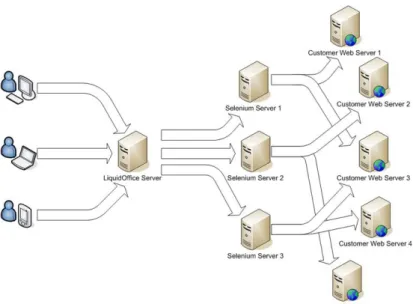
It is a data centric protocol that views the whole of the network as a large database [5]. It uses declarative query to abstract query processing. When generated data is huge, the architecture provides computation for energy efficiency.

(24)

14

Fig 2.4: Application of COUGAR in an internet network

 ACQUIRE

Its full name is ACtive QUery forwarding In sensoR nEtworks. It is similar to COUGAR and views the whole network as distributed database. The only difference is that it uses a look ahead parameter to take care of energy considerations.

 Energy Aware Routing (EAR)

Its primary objective is to increase the network lifetime. Its variation from directed diffusion is that it maintains a set of paths rather than an optimal path.

When different paths are chosen every single time, the energy of a single path won’t deplete early.

b. Hierarchical Network Routing

It is cluster based routing known for its scalability and efficient communication. It performs energy efficient routing by forming various clusters and giving special tasks to different cluster heads. It is basically a 2 layer process where;

 One layer is used to select cluster heads

(25)

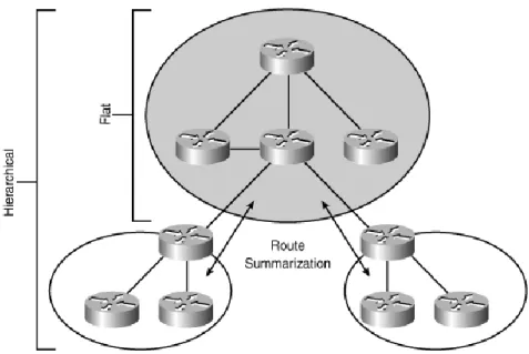
15

Fig 2.5: Difference between simple Flat and Hierarchical Routing

It is further sub divided into various protocols:-

 LEACH protocol

LEACH is a cluster based protocol that divides the sensors into small clusters for smooth functioning. It decides the cluster heads randomly. The periodical data collection is centralized. It is used for constant monitoring of data from physical environment like weather monitoring or observing an area for defense application.

(26)

16

 Power Efficient Gathering in Sensor Information Systems (PEGASIS)

It is an advanced version of LEACH protocol. The nodes mostly communicate with nearby nodes and in turns communicate directly with the BS. But unlike LEACH, it only uses one node to communicate with base station. It has 2 objectives;

 Increase the lifetime of each node

 Allow local communication between nearby nodes

 Threshold-sensitive Energy Efficient Protocols (TEEN and APTEEN)

These protocols are heavily used in time specific applications. The sensor senses frequently but the same rate is not maintained while sending the data. The cluster head sends;

 Hard threshold: Threshold value of sensed variable

 Soft threshold: Small change in variable that starts transmission

Fig 2.7: Time diagram for operation of TEEN and APTEEN

 Small Minimum Energy Communication Network (MECN)

It is a subnetwork that becomes a part of the main network. It works mainly to improve energy efficiency. It identifies relay region for every node that comprises of the neighboring nodes.

(27)

17

 Self-Organizing Protocol (SOP)

It is best suited for heterogeneous sensors. Works on both static as well as dynamic sensor. Router nodes are kept stationary. The data is forwarded to BS through these router nodes. It uses the Local Markov Loops (LML) algorithm to work by constructing spanning trees and traversing through them.

 Sensor Aggregates Routing

The objective is to collectively monitor target activity in a certain environment (target tracking applications). A sensor aggregate comprises those nodes in a network that satisfy a grouping predicate for a collaborative processing task. The parameters of the predicate depend on the task and its resource requirements.

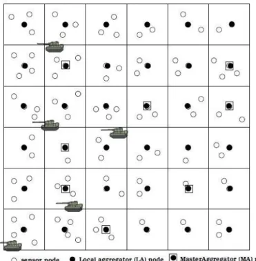
 Virtual Grid Architecture routing (VGA)

It works to improve energy efficiency and increase the lifetime of the network. It relies on data aggregation and in network processing of nodes to achieve the aims. It uses Integer Linear Program (ILP) algorithm to find the exact solutions.

(28)

18

 Hierarchical Power-aware Routing (HPAR)

The sensors are divided into groups called zones. These zones interact with each other but work on different methods to maximize the battery life. A zone graph is used to represent connected neighboring zone vertices if the current zone can go to the next neighboring zone in that direction.

 Two-Tier Data Dissemination (TTDD)

It provides the data packets to multiple mobile base stations. The data ports build a grid structure beforehand to send the data fast and efficiently through maximum throughput and minimum time delay. Sources are static but tail can be dynamic. Both are location aware.

c. Location Based Routing

In these routing techniques, the nodes are divided and addressed by means of their locations. The strength of the incoming signal or GPS can be used to determine the exact location of the nodes. The nodes can be programmed to go into sleep when they are inactive or dormant. The location based protocols are discussed in the subsections below:-



Geographic Adaptive Fidelity (GAF)

It is an energy aware and location based algorithm [6]. Its main application is in mobile ad hoc networks. The simplest explanation is made by the figure below;

(29)

19



Geographic and Energy Aware Routing (GEAR)

It uses energy and geographically concerned routing. This way it sends the data towards the BS. The main part is to consider only specific areas rather than the whole region. By doing this, GEAR can conserve more energy than directed diffusion.



MFR, DIR, and GEDIR

These protocols deal with basic distance, progress, and direction based methods. The key issues are forward direction and backward direction. A source node or any intermediate node will select one of its neighbors according to a certain criterion.



The Greedy Other Adaptive Face Routing (GOAFR)

It is a geometric ad hoc routing based on greedy and face algorithm. The greedy algorithm of GOAFR always picks the neighbor closest to a node to be next node for routing. However, it can be easily stuck at some local minimum, i.e. no neighbor is closer to a node than the current node.



SPAN

Based on the position of the nodes, few advantageous nodes are selected as coordinators [7]. It forms some sort of relay to forward the messages. Generally if two nodes cannot be connected directly, an in between node is made the coordinator.

2.3.2 Protocol Operation based Routing

These methods have different routing functions. They may be common with the above classified sections.

(30)

20

These protocols use high level data descriptors in order to eliminate redundant data transmissions through negotiation. Communication decisions are also taken based on the resources that are available to them. Hence, the main idea of negotiation based routing in WSNs is to suppress duplicate information and prevent redundant data from being sent to the next sensor or the BS by conducting a series of negotiation messages before the real data transmission begins.

b. Multi Path Based Routing

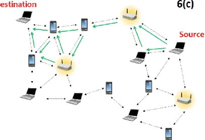
The fault tolerance (resilience) of a protocol is measured by the likelihood that an alternate path exists between a source and a destination when the primary path fails. This can be increased by maintaining multiple paths between the source and the destination at the expense of an increased energy consumption and traffic generation. These alternate paths are kept alive by sending periodic messages. Hence, network reliability can be increased at the expense of increased overhead of maintaining the alternate paths. The paths are chosen by means of a probability which depends on how low the energy consumption of each path is [8].

Fig 2.10: Example of Multipath based Routing

c. Query Based Routing

In this kind of routing, the destination nodes propagate a query for data (sensing task) from a node through the network and a node having this data sends the data which matches the query

(31)

21

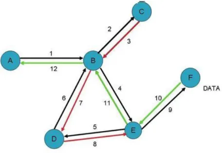
back to the node, which initiates the query. Usually these queries are described in natural language, or in high-level query languages.

Fig 2.11: Query based Routing with node weights

d. Coherent Based Routing

It generates large data amount. Hence scalability and energy efficiency must be achieved by optimal path.

e. QoS Based Routing

Quality of Service refers to quantitatively measure quality of service, several related aspects of the network service to be considered, such as error rates, bandwidth, throughput, transmission delay, availability, jitter, etc. Hence, there must be an optimization between energy consumption and data quality. Some data may be futile if it reaches beyond a certain time limit. QoS ensure this data integrity.

(32)

22

2.4

Comparison between various Routing Methods

Based on the above routing methods, they can be compared as follows:-

C√lassificatio n Mobility Position Awareness Power Usage Negotiation Based Data Aggregation Localization State Complexity

Scalability Multipath Query based

SPIN Flat Possible X Limite d

√ √ X Low Limited _√ _√

Directed Diffusion

Flat Limited X Limite d

√ √ √ Low Limited _√ _√

Rumor Routing

Flat Limited X N/A X _√ X Low Good X _√

GBR Flat Limited X N/A X _√ X Low Limited X _√

MCFA Flat X X N/A X X X Low Good X X

CADR Flat X X Limite

d

X _√ X Low Limited X X

COUGAR Flat X X Limite d

X _√ X Low Limited X _√

ACQUIRE Flat Limited X N/A X _√ X Low Limited X _√

EAR Flat Limited X N/A X _√ _√ Low Limited X _√

LEACH Hierarchical Fixed BS X Maxim um X X _√ CHs Good X X TEEN & APTEEN Hierarchical Fixed BS X Maxim um X _√ _√ CHs Good X X

PEGASIS Hierarchical Fixed BS X Maxim um X _√ X Low Good X X MECN & SMECN Hierarchical X X Maxim um X X X Low Low X X

SOP Hierarchical X X N/A X X X Low Low X X

HPAR Hierarchical X X N/A X X _√ Low Good X X

VGA Hierarchical X X N/A _√ X X CHs Good _√ X

Sensor Aggregate

Hierarchical Limited X N/A X _√ X Low Good X Possible TTDD Hierarchical Yes _√ Limite

d

X _√ X Moderate Low Possible Possible GAF Location Limited X Limite

d

X X X Low Good X X

GEAR Location Limited X Limite d

X X X Low Limited X X

SPAN Location Limited X N/A _√ X X Low Limited X X

MFR, GEDIR

Location X X N/A X X X Low Limited X X

GOAFR Location X X N/A X X X Low Good X X

SAR QoS X X N/A _√ _√ X Moderate Limited X _√

(33)

23

2.5 Conclusion

The present chapter presents various types of routing protocol based on Network Structure and Protocol Operation. There were further sub divisions which were explained by differentiating it with previous one. Finally, the chapter ends with the comparison between all of them so that the user can decide which technique to use as per the requirement. The further sections show a WSN based on Flat Network Routing and QoS based routing.

(34)

24

C H A P T E R

3

System Model for Simulation

Preface

This chapter describes the model of the system with the program and the attempt to simulate a WSN and find shortest paths and other parameters. The chapter also includes the flowchart and algorithm used to design the programs. The results are shown in the chapters following the present one.

(35)

25

3.1 Briefing of the simulation

The simulation can be done in MATLAB or Network Simulator. In this case, it is done in MATLAB R2012b. The overall simulation is divided into 2 parts:

-Creating the WSN -Analysis of the WSN

The first part loads a selected ad-hoc network from a given database structure and display its output. The database is a collection of the WSNs in the form of MATLAB matrices with the X, Y coordinates. The second part of the simulation shows the shortest path of the required node from each of the nodes. It then simulates the energy consumption of one round of data gathering from all the nodes.

Floyd Warshall algorithm is used to find out the shortest path between 2 nodes. It is present in the form of an inbuilt function which gives the shortest path from source to tail. The final vector includes the numbers of the vertices included in the shortest path from source to tail.

Its algorithm is as follows:- Start

Let Dist be a |N| × |N| array of minimum distances initialized to ∞ Let Dist_new be a |N| × |N| array of vertex indices initialized to null w (u,v)= direct connecting distance between u and v

For each edge (u,v) Dist[u][v] ← w(u,v) Dist_new [u][v] ← v For k from 1 to |N| For i from 1 to |N| For j from 1 to |N|

If Dist[i][k] + Dist[k][j] < Dist[i][j] then Dist[i][j] ← Dist[i][k] + Dist[k][j] Dist_new [i][j] ← Dist_new[i][k] Stop

(36)

26

3.2 Simulation of a WSN

3.2.1 Flowchart

Fig 3.1: Flowchart of WSN simulation Start

Select no of nodes (N), degree of nodes (d) and initialize R=25

Calculate ‘p’ from ‘d’ and ‘net’ from ‘p’

2 For Loops for fixed node and temporary nodes (1 to N)

Find difference between X, Y coordinates (𝑋₂-𝑋₁ and 𝑌₂-𝑌₁) and hence find the distance between the nodes d

Join the 2 nodes by a dashed line

End Is d > R

Yes

(37)

27 3.2.2 Program

(38)

(39)

29

3.3 Simulation for finding out various parameters

3.3.1 Flowchart

Fig 3.2: Flowchart of WSN parameter calculation Start

Enter no of nodes, grid/random topology, ID of receiver/base station

Initialize netM and RxTxM matrices to store X,Y coordinates

Plot the network and find the distances (as in previous case)

Find the shortest path of each node from receiver using Floyd Warshall algorithm

Modify the netM and RxTxM matrices with distances and the no of times each node is passed

Highlight the nodes of the shortest path on graph

Simulate one round of data gathering and plot it in a bar graph

(40)

30 3.3.2 Program

(41)

(42)

32

3.4 Conclusion

The programs were written in MATLAB R2012b and the simulation was done with varying number of nodes and degree of nodes. Further analysis of finding shortest path, measuring the distances, finding number of messages processed by each node, etc. were done. The results are shown in the following chapter.

(43)

33

C H A P T E R

4

Results and Outputs

Preface

This chapter shows all the graphs, calculated outputs, nodes involved in shortest path and the messages processed by each node along with the simulated WSN. The distances can be linked with time and QoS for specific applications can be obtained.

(44)

34

4.1 Output of WSN

4.1.1 Number of nodes = 50

Fig 4.1.1: Degree of nodes = 8

(45)

35 4.1.2 Number of nodes = 100

(46)

36 4.1.3 Number of nodes = 400

(47)

37

4.2 Output for shortest paths along with the distance

oneRoundWSN(100,0,25) R = 82.4621 sp = 1 25 dist = 93.5379 sp = 2 25 dist = 76.4931 sp = 3 25 dist = 101.7496 sp = 4 25 dist = 71.5157 sp = 5 25 dist = 66.2734 sp = 6 25 dist = 54.0950 sp = 7 25 dist = 35.3065 sp = 8 25 dist = 34.4256 sp = 9 25 dist = 28.7162 sp = 10 25 dist = 12.4583 sp = 11 25 dist = 21.2602 sp = 12 25 dist = 21.3675 sp = 13 25 dist = 42.8306 sp = 14 25 dist = 29.4877 sp = 15 25 dist = 15.7657 sp = 16 25 dist = 73.8098 sp = 17 25 dist = 93.6616 sp = 18 25 dist = 76.8885 sp = 19 25 dist = 45.4672 sp = 20 25 dist = 63.2276 sp = 21 25 dist = 53.8522 sp = 22 25 dist =39.8955 sp = 23 25 dist = 22.4152

(48)

38 sp = 24 25 dist = 41.6611 sp = 26 25 dist = 4.8886 sp = 27 26 25 dist = 8.6578 sp = 28 27 26 25 dist = 44.3433 sp = 29 28 27 26 25 dist = 47.1764 sp = 30 29 28 27 26 25 dist = 58.8216 sp = 31 25 dist = 92.9908 sp = 32 25 dist = 84.6193 sp = 33 25 dist = 89.6530 sp = 34 25 dist = 73.0261 sp = 35 25 dist = 60.6568 sp = 36 25 dist = 75.4269 sp = 37 25 dist = 56.2436 sp = 38 25 dist = 45.0080 sp = 39 25 dist = 49.2785 sp = 40 25 dist = 34.7307 sp = 41 33 25 dist = 158.5779 sp = 42 25 dist = 31.5580 sp = 43 34 25 dist = 170.5278 sp = 44 25 dist = 32.5746 sp = 45 35 25 dist = 123.0090 sp = 46 25 dist = 107.4340 sp = 47 36 25 dist = 122.0091 sp = 48 25 dist = 92.8353 sp = 49 37 25 dist = 76.6232 sp = 50 25 dist = 91.7946

(49)

39 sp = 51 25 dist = 84.9386 sp = 52 43 34 25 dist = 244.1166 sp = 53 25 dist = 68.0933 sp = 54 25 dist = 86.0790 sp = 55 45 35 25 dist = 182.0089 sp = 56 25 dist = 57.8592 sp = 57 25 dist = 58.3766 sp = 58 47 36 25 dist = 230.5822 sp = 59 25 dist = 72.8664 sp = 60 25 dist = 84.9996 sp = 61 52 43 34 25 dist = 312.0738 sp = 62 25 dist = 113.2820 sp = 63 44 25 dist = 135.9928 sp = 64 25 dist = 109.8126 sp = 65 55 45 35 25 dist = 224.0566 sp = 66 25 dist = 115.3638 sp = 67 46 25 dist = 162.2340 sp = 68 25 dist = 92.1418 sp = 69 58 47 36 25 dist = 287.9002 sp = 70 25 dist = 95.8842 sp = 71 25 dist = 99.0014 sp = 72 25 dist = 96.4786 sp = 73 25 dist = 101.6043 sp = 74 25 dist = 89.1615 sp = 75 65 55 45 35 25 dist = 291.5231

(50)

40 sp = 76 25 dist = 96.5402 sp = 77 25 dist = 53.2491 sp = 78 25 dist = 54.2947 sp = 79 25 dist = 81.1443 sp = 80 69 58 47 36 25 dist = 402.265 sp = 81 53 25 dist = 124.2793 sp = 82 63 44 25 dist = 251.8666 sp = 83 54 25 dist = 141.4345 sp = 84 25 dist = 3.5337 sp = 85 75 65 55 45 35 25 dist = 411.0526 sp = 86 25 dist = 80.0637 sp = 87 56 25 dist = 110.0983 sp = 88 67 46 25 dist = 193.6259 sp = 89 57 25 dist = 168.5435 sp = 90 25 dist = 116.2208 sp = 91 25 dist = 85.7231 sp = 92 25 dist = 49.3464 sp = 93 25 dist = 23.4650 sp = 94 25 dist = 111.8883 sp = 95 85 75 65 55 45 35 25dist = 499.0721 sp = 96 25 dist = 51.5406 sp = 97 25 dist = 35.5901 sp = 98 25 dist = 47.8035 sp = 99 25 dist = 15.8835 sp = 100 57 25 dist = 119.3719

(51)

41

4.3 Highlight of nodes involved in shortest path

It changes with every shortest path highlight the present path nodes. The last output has been stored in the dynamic graph. In this case, the last shortest path was from

1005725

Therefore, the nodes 100, 57, 25 are highlighted.

(52)

42

4.4 Bar graph for number of messages processed

Fig 4.5: Bar graph showing the number of messages processed by nodes

4.5 Conclusion

The above outputs were obtained from the simulation of the program. The distances from shortest path can be used to give time as speed of wireless communication is near to speed of light i.e. 3*108_{m/s. Hence, for a distance of 100m we get a time of transmission as 0.33µs.}

Similarly, the time required by all the paths can be found out and can be used to maintain a necessary quality like paths with transmission time less than 0.5µs.

(53)

43

C H A P T E R

5

Conclusion and Discussion

Preface

This chapter concludes the thesis by summarizing the details from Chapter 2 to Chapter 4. The highlighting points are mentioned and important points are discussed. Future scope of the WSN is also mentioned briefly.

(54)

44

5.1 Concluding points

Routing in sensor networks is a new area of research, with a limited, but rapidly growing set of research results. A Wireless Sensor Network consists of a number of node. It is plotted by considering a flat network and QoS factor. The number of nodes and degree of nodes is taken input from the user to plot the network on a 2-D graph. The distance are taken in meters. The thesis mainly focuses on shortest path because shortest path leads to shortest transmission time (ignoring the delay caused at the nodes), which in turn will lead to less energy consumption. A node was selected as the base station and the distance of all nodes from the BS were found out. The nodes contained in the shortest path were also mentioned. The results of the simulation can be clearly observed from the WSN simulated in 4.2. The node highlighting is done on a dynamic graph which changes when any new pair of nodes are taken into account. Further, the distances through the nodes are calculated (in meters) and presented alongside the shortest path. It can be used for comparative purposes.

5.2 Limitations of work

There are certain limitations to the thesis work. They are:-

 The nodes are considered static throughout the simulation. Extra complexity and difficulty have to be dealt with while considering movable/dynamic nodes.

 The simulation can be made only up to a certain number of nodes. Bigger networks can be time taking so must be simulated in other softwares.

 Energy requirement and supply are not taken into considerations. When these things are taken, the complexity of the network increases. These type of networks can be simulated using NS2 i.e. Network Simulator 2.

 A small example of QoS is taken based on distances. QoS base on transmission rate, energy, error, etc. cannot be done by this simulation.

(55)

45

5.3 Future work on thesis

Following are some of the directions of future works and research:-

 The comparison of various networks can be used for selection of the required network.

 The classification ad briefing of various routing protocol has been done. A mixture of 2 or more protocols can be used to give rise to a new type of WSN network satisfying more and more criteria.

 Study can be made to make node fault tolerant as generally, they tend to have a shorter lifetime.

 New techniques of Hierarchical routing are a hot topic in this field for research.

 Time synchronization should be considered as different nodes are at different distances from BS. This leads to a time delay even in same data being sensed. This can lead to erroneous results and must be taken care of.

(56)

46

References

[1] Jamal N. Al-Karaki, Ahmed E. Kamal "Routing Techniques in Wireless Sensor Networks", 2004

[2] J. Kulik, W. R. Heinzelman, and H. Balakrishnan, "Negotiation-based protocols for disseminating information in wireless sensor networks," Wireless Networks, Volume: 8, pp. 169-185, 2002.

[3] C. Intanagonwiwat, R. Govindan, and D. Estrin, "Directed diffusion: a scalable and robust communication paradigm for sensor networks," Proceedings of ACM MobiCom '00, Boston, MA, 2000, pp. 56-67.

[4] D. Braginsky and D. Estrin, "Rumor Routing Algorithm for Sensor Networks," in the Proceedings of the First Workshop on Sensor Networks and Applications (WSNA), Atlanta, GA, October 2002.

[5] Y. Yao and J. Gehrke, "The cougar approach to in-network query processing in sensor networks", in SIGMOD Record, September 2002.

[6] Y. Xu, J. Heidemann, D. Estrin,"Geography-informed Energy Conservation for Ad-hoc Routing," In Proceedings of the Seventh Annual ACM/IEEE International Conference on Mobile Computing and Networking 2001, pp. 70-84.

[7] B. Chen, K. Jamieson, H. Balakrishnan, R. Morris, "SPAN: an energy-efficient coordination algorithm for topology maintenance in ad hoc wireless networks", Wireless Networks, Vol. 8, No. 5, Page(s): 481-494, September 2002.

[8] C. Rahul, J. Rabaey, \Energy Aware Routing for Low Energy Ad Hoc Sensor Networks", IEEE Wireless Communications and Networking Conference (WCNC), vol.1, March 17-21, 2002, Orlando, FL, pp. 350-355.

[9] http://www.ieee802.org/15/

[10] F. Ye, A. Chen, S. Liu, L. Zhang, "A scalable solution to minimum cost forwarding in large sensor networks", Proceedings of the tenth International Conference on Computer Communications and Networks (ICCCN), pp. 304-309, 2001.

(57)

47

[11] W. Heinzelman, A. Chandrakasan and H. Balakrishnan, "Energy-Effcient Communication Protocol for Wireless Microsensor Networks," Proceedings of the 33rd Hawaii International Conference on System Sciences (HICSS '00), January 2000.

[12] F. Ye, H. Luo, J. Cheng, S. Lu, L. Zhang, "A Two-tier data dissemination model for large-scale wireless sensor networks", proceedings of ACM/IEEE MOBICOM, 2002.

[13] A. Patri, A. Nayak "A Fuzzy-Based Localization in Range-Free Wireless Sensor Network using Genetic Algorithm and Sinc Membership Function", In Green Computing, Communication and Conservation of Energy (ICGCE), 2013 International Conference on December, 2013, pp. 140-145.