www.elsevier.com/locate/tcs
Correlation clustering in general weighted graphs
夡
Erik D. Demaine
a,∗, Dotan Emanuel
b, Amos Fiat
b, Nicole Immorlica
a,1aComputer Science and Artificial Intelligence Laboratory, Massachusetts Institute of Technology, 32 Vassar Street, Cambridge, MA 02139, USA bDepartment of Computer Science, School of Mathematical Sciences, Tel Aviv University, Tel Aviv, Israel
Abstract
We consider the following generalcorrelation-clustering problem[N. Bansal, A. Blum, S. Chawla, Correlation clustering, in: Proc. 43rd Annu. IEEE Symp. on Foundations of Computer Science, Vancouver, Canada, November 2002, pp. 238–250]: given a graph with real nonnegative edge weights and a+/−edge labelling, partition the vertices into clusters to minimize the total weight of cut+edges and uncut−edges. Thus,+edges with large weights (representing strong correlations between endpoints) encourage those endpoints to belong to a common cluster while−edges with large weights encourage the endpoints to belong to different clusters. In contrast to most clustering problems, correlation clustering specifies neither the desired number of clusters nor a distance threshold for clustering; both of these parameters are effectively chosen to be the best possible by the problem definition. Correlation clustering was introduced by Bansal et al. [Correlation clustering, in: Proc. 43rd Annu. IEEE Symp. on Foundations of Computer Science, Vancouver, Canada, November 2002, pp. 238–250], motivated by both document clustering and agnostic learning. They proved NP-hardness and gave constant-factor approximation algorithms for the special case in which the graph is complete (full information) and every edge has the same weight. We give an O(logn)-approximation algorithm for the general case based on a linear-programming rounding and the “region-growing” technique. We also prove that this linear program has a gap of(logn), and therefore our approximation is tight under this approach. We also give an O(r3)-approximation algorithm for Kr,r-minor-free graphs. On the other hand, we show that the problem is equivalent to minimum multicut, and therefore APX-hard and difficult to approximate better than(logn).
© 2006 Elsevier B.V. All rights reserved.
Keywords:Clustering; Partitioning; Approximation algorithms; Minimum multicut
1. Introduction
Clusteringobjects into groups is a common task that arises in many applications such as data mining, web analysis, computational biology, facility location, data compression, marketing, machine learning, pattern recognition, and computer vision. Clustering algorithms for these and other objectives have been heavily investigated in the literature. For partial surveys, see e.g.[8,14,19–21,25].
In a theoretical setting, the objects are usually viewed as points in either a metric space (typically finite) or a general distance matrix, or as vertices in a graph. Typical objectives include minimizing the maximum diameter of a cluster
夡Preliminary versions of this paper appeared in APPROX 2003[6]and ESA 2003[7].
∗Corresponding author. Tel.: +1 617 253 6871; fax: +1 617 258 5429.
E-mail addresses:[email protected](E.D. Demaine),[email protected](D. Emanuel),fi[email protected](A. Fiat), [email protected](N. Immorlica).
1Research was supported in part by an NSF GRF.
0304-3975/$ - see front matter © 2006 Elsevier B.V. All rights reserved. doi:10.1016/j.tcs.2006.05.008
(k-clustering)[11], minimizing the average distance between pairs of clustered points (k-clustering sum) [24], mini-mizing the maximum distance to a “centroid object’’ chosen for each cluster (k-center) [11], minimizing the average distance to such a centroid object (k-median) [13], minimizing the average squared distance to an arbitrary centroid point (k-means) [14], and maximizing the sum of distances between pairs of objects in different clusters (maximum k-cut) [17]. These objectives interpret the distance between points as a measure of their dissimilarity: the larger the distance, the more dissimilar the objects. Another line of clustering algorithms interprets the distance or weights be-tween pairs of points as a measure of their similarity: the larger the weight, the more similar the objects. In this case, the typical objective is to find ak-clustering that minimizes the sum of weights between pairs of objects in different clusters (minimumk-cut) [17]. All of these clustering problems are parameterized by the desired numberkof clusters. Without such a restriction, these clustering objective functions would be optimized whenk =n(every object is in a separate cluster) or whenk=1 (all objects belong to a single cluster).
In thecorrelation-clustering problemintroduced by Bansal et al. [1], the underlying model is that objects can be truly categorized, and we are given probabilities about pairs of objects belonging to common categories. For example, the multiset of objects might consist of all authors of English literature, and two authors belong to the same category if they correspond to the same real person. This task would be easy if authors published papers consistently under the same name. However, some authors might publish under several different names such as William Shakespeare, W. Shakespeare, Bill Shakespeare, Sir Francis Bacon, Edward de Vere, and Queen Elizabeth I.2Given some confidence about the similarity and dissimilarity of the names, our goal is to cluster the objects to maximize the probability of correctness. There are two main objective functions for this problem: minimizing disagreements and maximizing agreements between the input estimates and the output clustering. The decision versions of these two optimization problems are identical and known to be NP-complete [1]. However, they differ in their approximability.
As we consider both similarity and dissimilarity measures in our problem, it is in a sense a generalization of the typical clustering objectives mentioned above. In fact, an appropriate interpretation of our problem instance suggests that our objective is a combination of the minimumk-clustering sum and minimumk-cut clustering objectives. An interesting property of our problem is that the numberkof clusters is no longer a parameter of the input; there is some “ideal’’kwhich the algorithm must find. Another clustering problem with this property islocation area design, a problem arising in cell phone network design. As formulated by Bejerano et al. [2], this problem attempts to minimize the sum of the squared sizes of the clusters plus the weight of the cut induced by the clustering. The similarities between these two problems allow us to apply many of the same techniques.
1.1. Our contributions
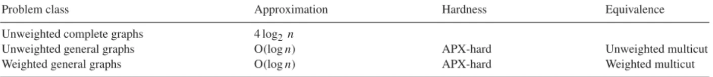
In this paper, we focus on the goal of minimizing disagreements in (weighted) general graphs. We give an O(log n)-approximation algorithm for weighted general graphs and an O(r3)-approximation algorithm for weighted graphs excluding the complete bipartite graphKr,r as a minor (e.g., graphs embeddable in surfaces of genus (r2)). Our O(logn)approximation is based on rounding a linear program using theregion growingtechnique introduced in the seminal paper of Leighton and Rao [17] on multicommodity max-flow min-cut theorems. Using ideas developed in Bejerano et al. [2], we are able to prove that this rounding technique yields a good approximation. Their paper also inspires our O(r3)approximation which uses a rounding technique introduced by Tardos and Vazirani [27] in a paper on max-flow min-multicut ratio and based on a lemma of Klein et al. [16]. We further prove that the gap in the linear program can be(logn), and therefore our bounds are tight for any algorithm based on rounding this linear program. We also prove that our problem is APX-hard because it is equivalent to the APX-hard problem of finding a minimum multicut [5], for which the current best approximation is O(logk)for a certain parameterk[9]. Any o(logn)-approximation algorithm for our problem would require improving the state-of-the-art for approximating minimum multicut. This equivalence also implies that any O(logk)algorithm for minimum multicut yields an O(logn) for correlation clustering. Our results are summarized in Table 1.
We remark that even for unweighted complete graphs, our (more general) algorithm has a better approximation ratio than the constant-factor approximation algorithm of [1] forn1081 ≈2270, a rough upper bound on the number of
2Some scholars believe William Shakespeare was actually a pen name for one of the wealthier and more renowned contemporaries of the Elizabethan era. Common candidates for the true authorship of Shakespeare’s works include Sir Francis Bacon, Edward de Vere, and even, on occasion, Queen Elizabeth I[23].
Table 1 Our contributions
Problem class Approximation Hardness Equivalence
Unweighted complete graphs 4 log2n
Unweighted general graphs O(logn) APX-hard Unweighted multicut
Weighted general graphs O(logn) APX-hard Weighted multicut
Table 2
Previous results on minimizing disagreements from[1]
Problem class Approximation Hardness
Unweighted complete graphs c≈20,000 NP-hard
Unweighted general graphs Open NP-hard
Weighted general graphs Open APX-hard
particles in the known universe. This is because their constant factor is approximately 20,000, whereas our approximation factor is smaller than 4 log2n.
Most of our results were obtained simultaneously and independently by Charikar et al.[3]. The results of their paper are detailed in the next section.
1.2. Related work
The only previous work on the correlation-clustering problem is that of Bansal et al. [1]. Their paper considers correlation clustering in an unweighted complete graph, i.e., every pair of objects has an estimate of either “similar’’ or “dissimilar’’. For minimizing disagreements, they give a constant-factor approximation via a combinatorial algorithm. For maximizing agreements, they give a polynomial-time approximation scheme (PTAS). The limitation of these two algorithms is that they assume the input graph is complete, while in many applications, estimate information is incomplete. Table 2 summarizes the results of their paper.
The constant-factor algorithm of Bansal et al. [1] for unweighted complete graphs is combinatorial. It iteratively “cleans’’ clusters until every clusterCis-clean(i.e., for every vertexv∈C,vhas at least(1−)|C|plus neighbors inCand at most|C|plus neighbors outsideC). They bound the approximation factor of their algorithm by counting the number of “bad’’ triangles (triangles with two+edges and one−edge) in a-clean clustering and use the existence of these bad triangles to lower bound OPT. Complete graphs have many triangles, and the counting arguments for counting bad triangles rely heavily on this fact. When we generalize the problem to graphs that are not necessarily complete, bad triangles no longer form a good lower bound on OPT. It may be possible to find a combinatorial algorithm for this problem that bounds the approximation factor by counting bad cycles (cycles with exactly one− edge). However, in this paper, we formulate the problem as a linear program and use theregion-growingtechnique to round it.
Simultaneously, and independent of our work, Charikar et al. [3] gave several algorithmic and hardness results for the correlation clustering problem. They studied both the minimization and maximization variants of the problem. For minimizing disagreements, they also formulated the problem as a linear program and used theregion-growingtechnique to round it. For complete graphs, they prove that this approach gives a factor 4 approximation. For general graphs, their O(logn)approximation is identical to ours. For both results, they investigate the integrality gap of the linear-programming formulation, finding examples with gaps of 2 and(logn), respectively. For maximizing agreements, the authors give a factor 0.7664 approximation in general graphs. As for hardness results, they prove APX-hardness of minimizing disagreements in complete graphs and maximizing agreements in general graphs. They also note that minimizing disagreements in general graphs is as hard as the minimum multicut problem.
Independent of Charikar et al. [3], the paper of Swamy [26] gives a 0.7666-approximation algorithm for the problem of maximizing agreements in general graphs. Recently, Charikar and Wirth [4] studied the problem of maximizing the correlation, or weight of agreements minus disagreements, of a clustering. Their paper details an (1/logn) approximation for this problem.
1.3. Paper structure
The rest of the paper is organized as follows. Section2 formalizes the correlation-clustering problem and some necessary notation. Section 3 presents explicit approximation algorithms for the problem in general andKr,r -minor-free graphs. Section 4 proves that the problem is equivalent to the minimum multicut problem, thus yielding an APX-hardness result and another implicit O(logn)algorithm. Section 5 discusses some applications of the correlation-clustering problem formulation. We conclude with open problems in Section 6.
2. Preliminaries
2.1. Problem definition
Bansal et al. [1] present the following clustering problem. We are given a graph onnvertices, where every edge (u, v)is labelled either +or −according to whetheru andv have been deemed to be similar or dissimilar. In addition, each edge has a weightce ∈ [0,∞)which can be interpreted as a confidence measure of the similarity or dissimilarity of the edge’s endpoints (higher weight denotes higher confidence).3 The goal is to produce a partition
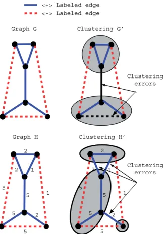
of the vertices (a clustering) that agrees as much as possible with the edge labels (see, for example, Fig. 1). More precisely, we want a clustering that maximizes the weight of agreements: the weight of+edges within clusters plus the weight of−edges between clusters. Alternatively, the clustering should minimize the weight of disagreements: the weight of−edges inside clusters plus the weight of+edges between clusters. Although the optimal solutions to these two problems are the same, they differ in their approximability.
In this paper, we focus on the problem of minimizing disagreements. In the rest of this paper when we refer to the “correlation-clustering problem’’ or “the clustering problem’’ we mean the problem of minimizing disagreements. We also say “positive edge’’ when referring to an edge labelled+and “negative edge’’ when referring to an edge labelled
−. Note that the terminology “positive’’ and “negative’’ here refers to the edge label and not the weight; edge weights are always nonnegative regardless of the label.
2.2. Notation
LetG=(V , E)be a graph onnvertices with edge weightsce0. Lete(u, v)denote the label (+,−) of the edge (u, v). LetE+ be the set of positive edges and letG+be the graph induced byE+,E+ = {(u, v)|e(u, v)=
+}, G+ =(V , E+). Likewise we defineE−andG−for negative edges.
In general, for a clusteringS= {S1, . . . , Sk}, letC(v)be the set of vertices in the same cluster asv. We call an edge (u, v)a positive mistake ife(u, v)= +and yetu /∈C(v). We call an edge(u, v)a negative mistake ife(u, v)= − andu∈C(v). The number of mistakes of a clusteringSis the sum of positive and negative mistakes. The weight of the clustering is the sum of the weights of mistaken edges inS. We introduce the following notation for the weight of a clusteringS: w(S)=wp(S)+wm(S), wp(S)= {ce :e=(u, v)∈E+, u /∈C(v)}, wm(S)= {ce :e=(u, v)∈E−, u∈C(v)}.
We refer to the optimal clustering as OPT and its weight or cost asw(OPT). For a general set of edgesT ⊂E, we define the weight ofTto be the sum of the weights inT,w(T )=e∈Tce. For a graphG=(V , E)and a set of edges T ⊂Ewe define the graphG\T to be the graph(V , E\T ).
3For example, if there is a functionf (u, v)that outputs the probability ofuandvbeing similar, then a natural assignment of weight to edge
Graph G Clustering G’ Clustering errors Graph H 5 5 5 5 1 2 1 2 2 5 5 5 5 1 2 1 2 2 Clustering H’ Clustering errors <+> Labeled edge <-> Labeled edge
Fig. 1. Two clustering examples for unweighted and weighted (general) graphs. In the unweighted case we give an optimal clustering with two errors: one error on an edge labelled+and one error on an edge labelled−. For the weighted case, we get a different optimal clustering with three errors on+edges and total weight 5.
3. O(logn)approximation
In this section, we use a linear-programming formulation of this problem to design an approximation algorithm. The algorithm first solves the linear program. The resulting fractional values are interpreted as distances between vertices; close vertices are most likely similar, far vertices are most likely dissimilar. The algorithm then uses region-growing techniques to group close vertices and thus round the fractional variables. Using ideas from Bejerano et al.[2], we are able to show that this approach yields an O(logn)approximation. We also present a modification to this approach that yields an O(r3)approximation forKr,r-minor-free graphs.
3.1. Linear-programming formulation
Consider assigning a zero-one variablexuv to each pair of vertices (hence xuv = xvu). When (u, v) ∈ E, we sometimes writexuvasxe where it is understood thate=(u, v). Given a clustering, setxuv =0 ifuandvare in a common cluster, andxuv =1 otherwise. To expressw(S)in this notation, note that 1−xeis 1 if edgeeis within a cluster and 0 if edgeeis between clusters. Thus
w(S)= e∈E− ce(1−xe)+ e∈E+ cexe.
Our goal is to find a valid assignment ofxuv’s to minimize this cost. An assignment ofxuv’s is valid (corresponds to a clustering) ifxuv∈ {0,1}and thexuv’s satisfy the triangle inequality.
We relax this integer program to the following linear program: minimize e∈E− ce(1−xe)+ e∈E+ cexe subject to xuv∈ [0,1], xuv+xvwxuw, xuv=xvu.
We will round this linear program to get an O(logn)approximation for our problem. This is in fact the best approximation factor that we can hope for with this linear program because it has an(log n)integrality gap.
Theorem 3.1. The integrality gap of the above linear program is(logn)in the worst case.
Proof. Recall that ad-regular graphG=(V , E)is a(d, c)-expanderif, for every subset of verticesUof size at most n/2,|N (U )|c|U|whereN (U )is the set of vertices inV \Uadjacent to vertices inU. Consider a(d, c)-expander Gfor some constantscandd, whose existence is shown in e.g.[22]. To construct our exampleG, set the weight of every edge inGto 1 and its label to+. For each vertexvinG, add an edge of weightnd/2 to all neighborsuwhose distance fromv is at least(logd(n/2)−1)/2. Set the label of these edges to−. Note that since there are at most nd/2 edges inG, the weight of a single−edge is at least the total weight of all+edges. Therefore, the optimal clusteringSmust cut all −edges, and so the diameters of the resulting clusters must be at most logd(n/2)−1. Because the vertices ofGhave bounded degreed, the size of the cluster of diameterris bounded bydr+1. Therefore, the clusters of the optimal clustering have size at mostn/2. By the expansion property ofG, the number of+edges we must cut is at least(cS∈S|S|)/2=(cn)/2, and so the weight of the optimal clustering is(n).
On the other hand, assigningxe = 2/(logd(n/2)−1) for +edges and xe = 1 for −edges is a feasible fractional solution of value at most(dn/2)×(2/(logd(n/2)−1)), and so the weight of the optimal fractional solution is O(n/logn). The theorem follows.
3.2. Rounding in general graphs 3.2.1. Region growing
We iteratively grow balls of at most some fixed radius (computed according to the fractionalxuv values) around nodes of the graph until all nodes are included in some ball. These balls define the clusters in the final approximate solution. As highxuvvalues hint thatuandvshould be in separate clusters, this approach seems plausible. The fixed radius guarantees an approximation ratio on disagreements within clusters while the region-growing technique itself guarantees an approximation ratio on disagreements between clusters.
First we present some notation that we need to define the algorithm. AballB(u, r)of radiusraround nodeuconsists of all nodesvsuch thatxuvr, the subgraph induced by these nodes, and the fraction(r−xuv)/xvwof edges(v, w) with only endpointv∈B(u, r). Thecutof a setSof nodes, denoted by cut(S), is the weight of the positive edges with exactly one endpoint inS, i.e.,
cut(S)=
|{v,w}∩S|=1, (v,w)∈E+ cvw.
Thecutof a ball is the cut induced by the set of vertices included in the ball. Thevolumeof a setSof nodes, denoted by vol(S), is the weighted distance of the edges with both endpoints inS, i.e.,
vol(S)=
{v,w}⊂S, (v,w)∈E+
cvwxvw.
Finally, thevolumeof a ball is the volume ofB(u, r)including the fractional weighted distance of positive edges leaving B(u, r). In other words, if(v, w)∈E+is a cut positive edge of ballB(u, r)withv∈B(u, r)andw /∈B(u, r), then (v, w)contributescvw·(r−xuv)weight to the volume of ballB(u, r). For technical reasons, we also include an initial volumeIto the volume of every ball (i.e., ballB(u,0)has volumeI).
3.2.2. Algorithm
We can now present the algorithm for rounding a fractional solution FRAC to an integral solution SOL. Suppose the volume of the entire graph isF, and thuswp(FRAC)=F. Let the initial volumeIof the balls defined in the algorithm beF /n, and letcbe some constant which we determine later.
AlgorithmRound
(1) Pick any nodeuinG. (2) Initializerto 0.
(3) Growrby min{(duv−r) > 0 : v /∈ B(u, r)}so that B(u, r)includes another entire edge, and repeat until cut(B(u, r))cln(n+1)×vol(B(u, r)).
(4) Output the vertices inB(u, r)as one of the clusters inS. (5) Remove vertices inB(u, r)(and incident edges) fromG. (6) Repeat Steps 1–5 untilGis empty.
This algorithm clearly runs in polynomial time and terminates with a solution that satisfies the constraints. We must show that the resulting cost is not much more than the original fractional cost. Throughout the analysis section, we refer to the optimal integral solution as OPT. We also use FRAC(xuv)and SOL(xuv)to denote the fractional and rounded solution of the variablexuvin the linear program.
3.2.3. Positive edges
The termination condition on the region-growing procedure guarantees an O(logn)approximation to the cost of positive edges (between clusters). LetBbe the set of balls found by our algorithm in step 3. Then,
wp(SOL)= (u,v)∈E+ cuvSOL(xuv) = 1 2 B∈B cut(B) c 2ln(n+1)× B∈B vol(B) c 2 ln(n+1)× (u,v)∈E+ cuvFRAC(xuv)+ B∈B F n c 2 ln(n+1)× wp(FRAC)+F cln(n+1)×wp(FRAC),
where the fourth line follows from the fact that the balls found by the algorithm are disjoint.
The rest of our analysis hinges on the fact that the balls returned by this algorithm have radius at most 1/c. This fact follows from the following known lemma[28]:
Lemma 3.2. For any vertex u and any family of ballsB(u, r),the conditioncut(B(u, r))cln(n+1)×vol(B(u, r)) is achieved for somer1/c.
3.2.4. Negative edges
As in Bejerano et al. [2], we can use this radius guarantee to bound the remaining component of our objective function. We see that our solution gives ac/(c−2)-approximation to the cost of negative edges (within clusters). Again, letBbe the set of balls found by our algorithm in step 3. Then,
wm(FRAC)= (u,v)∈E− cuv(1−FRAC(xuv)) B∈B (u,v)∈B∩E− cuv(1−FRAC(xuv))
B∈B (u,v)∈B∩E− cuv(1−2/c) (1−2/c) B∈B (u,v)∈B∩E− cuv = c−2 c wm(SOL),
where the third line follows from the triangle inequality and the 1/cbound on the radius of the balls. The approximation ratioc/(c−2)is O(1)providedc >2.
3.2.5. Overall approximation
Combining these results, we pay a total of w(SOL)=wp(SOL)+wm(SOL)
cln(n+1)×wp(OPT)+ c c−2 ×wm(OPT) max cln(n+1), c c−2 w(OPT)
and thus we have an O(lnn)approximation, where the lead constant,c, is just slightly larger than 2.
3.3. Rounding inKr,r-minor-free graphs
InKr,r-minor-free graphs, we can use a theorem of Klein et al.[16] to round our linear program in a way that
guarantees an O(r3) approximation to the cost of disagreements between clusters. The clusters produced by this rounding have radius at most 1/c, and thus the rest of the results from the previous section follow trivially. The theorem states that, in graphs with unit-length edges, there is an algorithm to find a “small’’ cut such that the remaining graph has “small’’ connected components:
Theorem 3.3(Klein et al.[16]). In a graph G with weight u on the edges which satisfy the triangle inequality,one can find in polynomial time either aKr,r minor or an edge cut of weightO(rU/)whose removal yields connected
components of weak diameter4 O(r2)where U is the total weight of all edges in G.
As in the case of the region-growing technique, this theorem allows us to cluster the graph cheaply, subject to some radius guarantee. As this clustering cost is independent ofn, this technique is typically applied in place of the region-growing technique to get better approximations forKr,r-minor-free graphs. (see, for example, Tardos and Vazirani [27] or Bejerano et al. [2]) In particular, this implies constant-factor approximations for various clustering problems on planar graphs.
The idea is as follows. Given aKr,r-minor-free graphGwith weightsceand edge lengthsxeas defined by the linear program, we subdivide each edgee∈E+(G)into a chain ofkxeedges of the same weightcefor some appropriate k, yielding a new graphG. (Note that we do not include the negative edges ofGinG.) We apply Theorem 3.3 to G, getting an edge cutFwhich maps to an edge cutF inGof at most the same weight. This creates the natural correspondence between the resulting components ofGandG. Note two nodes at distancedinGare at distance at leastkdinG. Hence, if we take=O(k/(cr2)), for a sufficient setting of the constants the components inGwill have diameter at most 2/c.
For any constantc >2, we can bound the weight of the negative mistakes as in Section 3.2 by(c/(c−2))wm(FRAC). The weight of the positive mistakes is simply the weight of the cutF, and so, by Theorem 3.3, we just need to bound the total weightU of the graphG. LetU = e∈E+(G)ce be the total weight of positive edges in Gand 4Theweak diameterof a connected component in a modified graph is the maximum distance between two vertices in that connected component as measured in the original graph. For our purposes, distances are computed according to thexu,vwhich satisfy the triangle inequality and are
recall vol(G)=e∈E+(G)cexe. Then U= e∈G ce = e∈E+(G) kxece e∈E+(G) (kxe+1)ce =kvol(G)+U.
By Theorem3.3, the weight of F, which equals the weight ofF, is O(rU/) = O(r3(kvol(G)+U )/ k). Taking k=U/vol(G), this becomes O(r3vol(G))and is thus an O(r3)approximation of the cost of disagreements between clusters, as desired. The size ofGmay be pseudo-polynomial in the size ofG. However, the algorithm of Klein et al. [16] consists ofrbreath-first searches ofG, and these can be implemented without explicitly subdividingG. Thus, the algorithm runs in polynomial time.
4. Relation to multicut
In this section, we prove that the correlation-clustering problem is equivalent to the multicut problem, thus yielding another O(logn)approximation for our problem as well as some hardness results.
Definition 4.1. Theweighted multicut problemis the following: given an undirected graphG, a weight functionwon the edges ofG, and a collection ofkpairs of distinct vertices(si, ti)ofG, find a minimum weight set of edges ofG whose removal disconnects everysifrom the correspondingti.
The multicut problem was first stated by Hu in 1963[12]. Fork =1, the problem coincides, of course, with the ordinary min-cut problem. Fork = 2, it can be also solved in polynomial time by two applications of a max flow algorithm [31]. The problem was proven NP-hard and APX-hard for any k3 in by Dahlhaus et al. [5]. The best known approximation ratio for weighted multicut in general graphs is O(logk)[9] . For planar graphs, Tardos and Vazirani [27] give an approximate max-flow min-cut theorem and an algorithm with a constant approximation ratio. For trees, Garg et al. [10] give an algorithm with an approximation ratio of 2.
4.1. Reduction from correlation clustering to weighted multicut
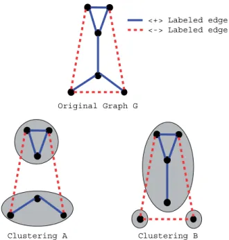
We now show that finding an optimal clustering is equivalent to finding a minimum-weight edge set that covers all erroneous cycles. Anerroneous cycleis a simple cycle containing exactly one negative edge. An edgecoversa cycle if the edge is contained in the cycle, i.e., removing the edge breaks the cycle. Fig. 2 illustrates the equivalence.
Guided by this observation, we define a multicut problem derived from our original graph by replacing the negative edges with source-sink pairs (and some other required changes). We show that a solution to the newly formed multicut problem induces a solution to the clustering problem with the same weight, and that optimal solution to the multicut problem induces an optimal solution to the clustering problem.
These reductions imply that the O(logk)-approximation algorithm for the multicut problem [9] induces an O(log n)-approximation algorithm for the correlation-clustering problem. We prove this for weighted general graphs, which implies the same result for unweighted general graphs. We start by proving two simple lemmata. We call a clustering aconsistent clusteringif it contains no mistakes, i.e., if there are no cut positive edges or uncut negative edges. Lemma 4.2. A graph contains no erroneous cycles if and only if it has a consistent clustering.
Proof. LetGbe a graph with no erroneous cycles, and letSbe the set of connected components ofG+. We argue that
Original Graph G
Clustering A Clustering B <+> Labeled edge <-> Labeled edge
Fig. 2. Two optimal clusterings forG. For both of these clusterings we have removed two edges (different edges) so as to eliminate all the erroneous cycles inG. After the edges were removed every connected component ofG+is a cluster. Note that the two clusterings are consistent; no positive edges connect two clusters and no negative edges connect vertices within the same cluster.
uandvbelong to the same cluster, they are on the same connected component ofG+. It follows that there is a simple path of positive edges fromutov. This path, combined with the negative edge(u, v), creates an erroneous cycle. From the construction ofS(the connected components ofG+) it is obvious thatScontains no positive mistakes either, and soSis a consistent clustering.
LetSbe a consistent clustering on a graphG. We claim thatGcontains no erroneous cycles. Assume(v1, v2, . . . , vk) is an erroneous cycle of sizek. Without loss of generality, we let(v1, v2)be the negative edge in the cycle. Ifv1∈C(v2)
then we have a negative mistake which meansSis not consistent. Ifv1∈/C(v2)then there must exist a point 1ik−1
along the cycle such thatvi ∈/C(vi+1)which in turn means that the edge(vi, vi+1)is a positive mistake. Lemma 4.3. Let F be a set of edges of minimum weight such thatG\F contains no erroneous cycles and T be a set of edges on which an optimal clustering makes mistakes. Then the weight of F equals the weight of T.
Proof. LetSbe a clustering onG, and letTbe the set of mistakes made by this clustering. ThenSis a consistent clustering onG\T, and so the result follows from Lemma4.2.
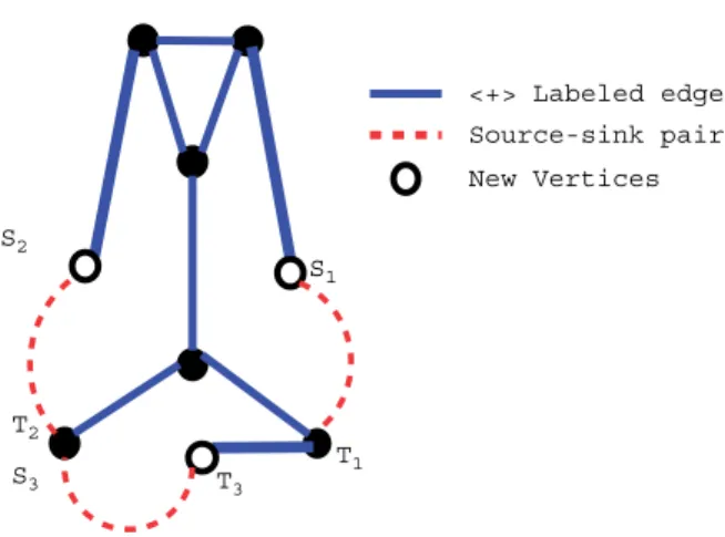
We give a reduction from the problem of correlation clustering to the weighted multicut problem. The reduction translates an instance of unweighted correlation clustering into an instance of unweighted graph multicut, and an instance of weighted correlation clustering into an instance of weighted graph multicut. Refer to Fig. 3 for an example.
Given a weighted graphGwhose edges are labelled{+,−}, we construct a new graphHG and a collection of source-sink pairsSG= {si, ti}as follows:
• For every negative edge(u, v)∈E−we introduce a new vertexvu,v, a new edge(vu,v, u)with weight equal to that of(u, v), and a source-sink pairvu,v, v.
• Let Vnew denote the set of new vertices, Enew, the set of new edges, andSG, the set of source-sink pairs. Let V=V ∪Vnew,E=E+∪Enew,HG=(V, E). The weight of the edges inE+remains unchanged. We now have a multicut problem on(HG, SG).
We claim that any solution to the multicut problem implies a solution to the correlation-clustering problem with the exact same value, and that an approximate solution to the former gives an approximate solution to the latter.
Transformed graph H S1 T1 S2 S3 T2 T3 <+> Labeled edge Source-sink pair New Vertices
Fig. 3. The original graph from Fig.2after the transformation.
Theorem 4.4. (HG, SG)has a cut of weightW if and only if G has a clustering of weightW,and we can easily
construct one from the other. In particular,the optimal clustering in G of weightW implies an optimal multicut in (HG, SG)of weightWand vice versa.
The proof follows from the following two lemmas:
Lemma 4.5. LetSbe a clustering on G with weightW.Then there exists a multicutTin(HG, SG)with weightW.
Proof. LetSbe a clustering ofG with weightW, whereTis the set of mistakes made by S(w(T ) = W). Let T =(T ∩G+)∪ {(vu,v, u)| (u, v)∈ T ∩G−}. Note thatw(T ) =w(T). We now argue thatTis a multicut. Assume not; then there exists a pair(vu,v, v) ∈ SG and a path from vu,v tou that contains no edge fromT. By construction, this implies that there exists a path fromutovinG+\T which, together with the negative edge(u, v), forms an erroneous cycle inG\T. This is a contradiction since, by definition ofT,G\T has a clustering with no mistakes. Note that the proof is constructive.
Lemma 4.6. IfTis a multicut in(HG, SG)of weightW,then there exists a clusteringSin G of weightW.
Proof. We construct a setTfrom the cutTby replacing all edges inTthat are inEnewwith the corresponding negative
edges inG, and define a clusteringSby taking every connected component ofG+\T as a cluster. Note thatThas the same total weight asT. We argue thatTis precisely the set of mistakes ofS, and thus the weight ofSisW. In other words, it suffices to prove thatSis a consistent clustering onG\T. Assume not; then there exists an erroneous cycle inG\T (Lemma4.2). Let(u, v)be the negative edge along this cycle. Then it follows that there is a path fromvu,v tovinHGwhich does not traverse any edge inT. But the pairvu,v, vis a source-sink pair which is in contradiction toTbeing a multicut.
We have presented a mapping ffrom an instancexof the correlation-clustering problem to an instance f (x)of the multicut problem. We have also presented a mappinggfrom a feasible solution off (x)(multicut problem) to a feasible solution ofx(the clustering problem) such that the value of the solution does not change. This means that if sis a solution to the multicut problemf (x)such thatw(s)=O(·w(OPT(Multicut)))theng(s)is a solution to the clustering problem such thatw(g(s))=·w(OPT(Clustering)). We can now use the approximation algorithm of [9] to get an O(logk)approximation solution to the multicut problem (kis the number of source-sink pairs) which translates into an O(log|E−|)O(logn2)=O(logn)solution to the clustering problem. Note that this result holds for both weighted and unweighted graphs and that the reduction of the unweighted correlation-clustering problem results in a multicut problem with unit capacities and demands.
4.2. Reduction from multicut to correlation clustering
In the previous section, we showed that every correlation-clustering problem can be presented (and approximately solved) as a multicut problem. We now show that the opposite is true as well, that every instance of the multicut problem can be transformed to an instance of a correlation-clustering problem, and that transformation has the following properties: any solution to the correlation-clustering problem induces a solution to the multicut problem with lower or equal weight, and an optimal solution to the correlation-clustering problem induces an optimal solution to the multicut problem.
In the previous section, we could use one reduction for the weighted version and the unweighted version. Here, we present two slightly different reductions from unweighted multicut to unweighted correlation clustering and from weighted multicut to weighted correlation clustering.
4.2.1. Reduction from weighted multicut to weighted correlation clustering
Given a multicut problem instance: an undirected graphH, a weight functionwon the edges ofH,w:E →R+, and a collection ofkpairs of distinct verticesS = {si, ti, . . . ,sk, tk)}ofH, we construct a correlation-clustering problem as follows:
• We start withGH =H, all edge weights are preserved and all edges labelled+.
• In addition, for every source-sink pair si, tiwe add to GH a negative edgeei = (si, ti)with weightw(ei) = e∈Hw(e)+1.
Our transformation is polynomial, adds at most O(n2) edges, and increases the largest weight in the graph by a multiplicative factor of at most O(n2).
Theorem 4.7. A clustering onGH with weightW induces a multicut on(H, S)with weight at mostW.Similarly,a
multicut in(H, S)with weightWinduces a clustering onGH with weightW.
Proof. LetSbe a clustering onGHof weightW. IfScontains no negative mistakes, then the set of positive mistakes
Tis a multicut onHof weightW. IfScontains a negative mistake, say(u, v), take one of the endpoints (uorv) and place it in a cluster of its own, thus eliminating this mistake. Because every negative edge has weight at least the sum of all positive edges, the gain by splitting the cluster exceeds the loss introduced by new positive mistakes. Therefore, the new clusteringSonGhas weightW< W, and contains no negative mistakes. Thus, the set of positive mistakes Tis a multicut onHof weight at mostW.
Now, letTdenote a multicut in(H, S)of weightWand define clusteringSonGH as the connected components of G+\T. Note thatScontains no negative mistakes and so has weightw(T )=W.
Corollary 4.8. An optimal clustering inGH induces an optimal multicut in(H, S).
Proof. This follows directly from the statements in the above lemma.
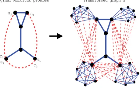
4.2.2. Reduction from unweighted multicut to unweighted correlation clustering
Given an unweighted multicut problem instance: an undirected graphHand a collection ofkpairs of distinct vertices S= {si, ti, . . . ,sk, tk}ofH, we construct an unweighted correlation-clustering problem as follows; refer to Fig.4.
• For everyvsuch thatv, u ∈Soru, v ∈S(i.e.,vis either a source or a sink), we addn−1 new vertices and connect those vertices andvin a clique with positive edges (weight 1). We denote this clique byQv.
• For every pairsi, ti ∈S, we connect all vertices ofQsi toti and all vertices ofQti tosiusing edges labelled−.
• Other vertices of Hare added to the vertex set of GH, and edges of Hare added to the edge set of GH and labelled+.
Our goal is to emulate the previous argument for weighted general graphs in the context of unweighted graphs. We do so by replacing the single edge of high weight with many unweighted negative edges. Our transformation needs polynomial time, and it adds at mostn2vertices and at most O(n3)edges.
Lemma 4.9. Given a clustering C on G,we can construct another clustering C on G such thatC is pure and w(C)w(C).
Original Multicut problem Transformed graph G S1 T1 S2 S3 T2 T3
Fig. 4. Transformation from the unit-capacity multicut problem (on the left) to the unweighted correlation-clustering problem (on the right).
Proof. For everyQvthat is split amongst two or more cluster we take all vertices ofQvto form a new cluster. By doing so, we may be adding up ton−1 new mistakes, (positive mistakes, positive edges adjacent tovin original graph). Merging these vertices into one cluster component reduces the number of errors by at leastn−1.
If twoQv andQw are in the same cluster component, we can move one of them into a cluster of its own. As before, we may be introducing as many asn−1 new positive mistakes but simultaneously eliminating 2nnegative mistakes.
Theorem 4.10. A clustering onGHwith weightWinduces a multicut on(H, S)with weightW.An optimal clustering
in G of weightWinduces an optimal multicut for(H, S)of weightW.
Proof. We call a clustering pure if all vertices that belong to the sameQvare in the same cluster, and that ifv, w ∈S thenQvandQware in different clusters. The following proposition states that we can “fix’’ any clustering to be a pure clustering without increasing its weight.
Given a clusteringConGH we first “fix’’ it using the technique of Lemma4.9 to obtain a pure clusteringC. Any
mistake for pure clustering must be a positive mistake, the only negative edges are between clusters.
LetTbe the set of positive mistakes forC, we now show thatTis a multicut on(H, S). No source-sink pair are in the same cluster because the clustering is pure and removing the edges ofTdisconnects every source/sink pair. Thus, Tis a multicut for(H, S).
Let OPT be the optimal clustering onG. Without loss of generality, we can assume that OPT is pure (otherwise, by Lemma 4.9, we can construct another clustering with no higher cost) and therefore induces a multicut on(H, S). Let Tdenote the minimum multicut in(H, S).Tinduces a pure-clustering onGas follows: take the connected component ofG+\T as clusters and for every terminalv ∈Sadd every node inQvto the cluster containing verticesv. It can be easily seen that this gives a pure clustering, and that the only mistakes on the clustering are the edges inT. The result follows.
4.3. Remarks
The two-way reduction we just presented proves that the correlation-clustering problem and the multicut problem are essentially identical. This reduction also allows us to transfer hardness-of-approximation results from one problem to the other. Because the multicut problem is APX-hard and remains APX-hard even in the unweighted case, the unweighted correlation-clustering problem is also APX-hard.
An interesting observation comes from the constant-factor approximation for the correlation clustering problem on the unweighted complete graph from[1]. This result implies that the corresponding unweighted multicut problem, in which every pairu, vof nodes is either an edge or a source-sink pair, has a constant-factor approximation.
On the other hand, correlation-clustering problems whereG+ is a planar graph or has a tree structure has a constant-factor approximation (as follows from [27,10]).
5. Use of correlation clustering
In this section, we motivate correlation clustering by describing several clustering situations where it is useful. 5.1. When we have attraction/rejection data
The correlation-clustering approach gives us a natural and unique way to solve problems that have more than one distance measure or problems that need to balance between two possible contradicting measures. For example, suppose we have a set of guests, each of whom has preferences for people they would like to sit with and for people they would prefer to avoid. We must group the guests into tables in a way that enhances amicability of the atmosphere. Using the correlation-clustering setting we can solve this problem and get a provable approximation bound.
5.2. As a way of solving constraint-clustering problems
There has been a great deal of work on solving clustering problems subject to constraints [18,29,30,15]. In a constraint clustering problem we have the following inputs:
(1) A set of objects, a distance measure between them, and an objective function to be minimized (the traditional clustering setting).
(2) A set of pairwise constraints among the objects.
One seeks a clustering that minimizes the objective function and satisfies the set of constraints simultaneously. One common approach to address constraint-clustering problems is to use a clustering/search algorithm (e.g.,k-means[18], k-median, hierarchical clustering) in the space of all feasible clusterings (those respecting the constraint). This approach treats the constraints as hard and consistent (must and can be simultaneously satisfied), and assumes that one can search through the space of feasible constraints [29,30,15].
We suggest a different approach: instead of treating a constraint-clustering problem as an unconstrained clustering problem in a trimmed search space, we look at the problem as a soft constraint satisfaction problem. We convert the distance between any two items into a constraint, combine this set of constraints with the original set of constraints and solve the resulting constraint satisfaction problem. Restructuring the problem as a constant satisfaction problem allows us to use the correlation-clustering algorithm and get a provable approximation result as opposed to the search heuristics used in previous constrained clustering algorithms.
5.3. As a way to determine the number of clusters
Traditional clustering methods use positive distance or similarity measures and seek to minimize the distance or maximize the similarity of elements within the same cluster. To avoid the problem of converging to the trivial solutions of putting all elements in the same cluster (maximize similarity) or putting each element in a cluster of his own, (minimize distances within a cluster), one usually limits the number of clusters. (e.g.,k-means,k-median, etc.).
Correlation clustering suggests a different approach. Given a distance measure, we set a threshold, where all distances below the threshold represent attraction (the elements are close, they should be in the same cluster) and distance above the threshold represents rejection (the elements are far apart, they should not be in the same cluster). We create a graph were each item is a node and between any two elements we have an edge. We label these edges+if the distance between the elements is below the threshold and−if it is above the threshold. We set the weight of the edge according to the original distance between the elements; small distances become a positive labelled edges with large weight, whereas large distance become negative labelled edges of large weight. We now solve the correlation-clustering problem on the resulting graph.
One advantage of this approach is that choosing a threshold can be much more meaningful then choosing the number of clusters. The threshold is a property of the distance measure; it is just our observation of “near’’ and “far’’. It is independent of the actual data, and therefore, unlike an arbitrary number of clusters,k, may have a “real’’ meaning. Another possible advantage of this approach is that the correlation-clustering algorithm can also handle outliers easily. Outliers will usually get a cluster of their own, and when the algorithm ends we can simply discard small isolated clusters.
5.4. When we have only partial pairwise measures
Mostk-based algorithms assume points are positioned in a metric space, or at least that we have a known weight for every pair of items. This is usually not the case in real-world problems. When using the correlation-clustering framework we can work with any subset of pairwise distance measure and just omit the unknown relations from the graph.
6. Conclusion
In this paper, we have investigated the problem of minimizing disagreements in the correlation-clustering problem. We gave an O(logn)approximation for general graphs, an O(r3)approximation forKr,r-minor-free graphs, and showed that the natural linear-programming formulation upon which these algorithms are based has a gap of(logn)in general graphs. We also showed that this problem is equivalent to the minimum multicut, yielding another implicit O(logn) approximation as well as an APX-hardness result.
A natural extension of this work would be to improve the approximation factor for minimizing disagreements. Given our hardness result and the history of the minimum-multicut problem, this goal is probably very difficult. Another option is to improve the lower bound, but for the same reason, this goal is probably very difficult. On the other hand, one might try to design an alternate O(logn)-approximation algorithm that is combinatorial, perhaps by counting erroneous cycles in a cycle cover of the graph.
Another interesting direction is to explore other objective functions of the correlation-clustering problem. Bansal et al.
[1] give a polynomial-time approximation scheme (PTAS) for maximizing agreements in unweighted complete graphs. For weighted general graphs, one of two trivial clusterings (every vertex in a distinct cluster or all vertices in a single cluster) is a12approximation. Recently, Swamy [26] gave a 0.7666-approximation algorithm for the unweighted general graphs based on semidefinite programming. It would be interesting to obtain better approximations, in particular a PTAS, for general graphs. Bansal et al. [1] also mention the objective of maximizing agreements minus disagreements. This objective is of particular practical interest. However, there are no known approximation algorithms for this objective, even for complete graphs.
Finally, it would be interesting to apply the techniques presented here to other problems. The region-growing technique and Klein et al. [16] rounding technique both provide a radius guarantee on the output clusters. Many papers have used this radius guarantee to demonstrate that the solution isfeasible, i.e., satisfies the constraints. Inspired by Bejerano et al. [2], we also use the radius guarantee tobound the approximation factor. This idea might be applicable to other problems.
Acknowledgments
Many thanks go to Avrim Blum, Shuchi Chawla, Mohammad Mahdian, David Liben-Nowell, and Grant Wang for helpful discussions. Many results in this paper were inspired by conversations with Seffi Naor.
References
[1]N. Bansal, A. Blum, S. Chawla, Correlation clustering, in: Proc. 43rd Annu. IEEE Symp. on Foundations of Computer Science, Vancouver, Canada, November 2002, pp. 238–250.
[2]Y. Bejerano, N. Immorlica, J. Naor, M. Smith, Efficient location area planning for personal communication systems, in: Proc. Ninth Annual Internat. Conf. on Mobile Computing and Networking, San Diego, CA, September 2003, pp. 109–121.
[3]M. Charikar, V. Guruswami, A. Wirth, Clustering with qualitative information, in: Proc. 44th Annu. IEEE Symp. Foundations of Computer Science, 2003, pp. 524–533.
[4]M. Charikar, A. Wirth, Maximizing quadratic programs: extending grothendieck’s inequality, in: Proc. 45th Annu. IEEE Symp. on Foundations of Computer Science, 2004, pp. 54–60.
[5]E. Dahlhaus, D.S. Johnson, C.H. Papadimitriou, P.D. Seymour, M. Yannakakis, The complexity of multiterminal cuts, SIAM J. Comput. 4 (23) (1994) 864–894.
[6]E.D. Demaine, N. Immorlica, Correlation clustering with partial information, in: Proc. Sixth Internat. Workshop on Approximation Algorithms for Combinatorial Optimization Problems, Princeton, NJ, August 2003, pp. 1–13.
[7]D. Emanuel, A. Fiat, Correlation clustering—minimizing disagreements on arbitrary weighted graphs, in: Proc. 11th Annu. European Symp. on Algorithms, 2003, pp. 208–220.
[8]M. Ester, H.-P. Kriegel, J. Sander, X. Xu, Clustering for mining in large spatial databases, KI-Journal 1 (1998) 18–24 (Special Issue on Data Mining. ScienTec Publishing).
[9]N. Garg, V.V. Vazirani, M. Yannakakis, Approximate max-flow min-(multi)cut theorems and their applications, SIAM J. Comput. 25 (2) (1996) 235–251.
[10]N. Garg, V.V. Vazirani, M. Yannakakis, Primal-dual approximation algorithms for integral flow and multicut in trees, Algorithmica 18 (1) (1997) 3–20.
[11]D.S. Hochbaum, D.B. Shmoys, A unified approach to approximation algorithms for bottleneck problems, J. ACM 33 (1986) 533–550.
[12]T.C. Hu, Multicommodity network flows, Oper. Res. 11 (1963) 344–360.
[13]K. Jain, V.V. Vazirani, Primal-dual approximation algorithms for metric facility location andk-median problems, in: Proc. 40th Annu. Symp. on Foundations of Computer Science, 1999, pp. 2–13.
[14]T. Kanungo, D.M. Mount, N.S. Netanyahu, C.D. Piatko, R. Silverman, A.Y. Wu, An efficientk-means clustering algorithm: analysis and implementation, IEEE Trans. Pattern Anal. Mach. Intell. 24 (7) (2002) 881–892.
[15]D. Klein, S.D. Kamvar, C.D. Manning, From instance-level constraints to space-level constraints: making the most of prior knowledge in data clustering, in: Proc. 19th Internat. Conf. on Machine Learning, 2002, pp. 307–314.
[16]P.N. Klein, S.A. Plotkin, S. Rao, Excluded minors, network decomposition, and multicommodity flow, in: Proc. 25th Annu. ACM Symp. on Theory of Computing, 1993, pp. 682–690.
[17]T. Leighton, S. Rao, Multicommodity max-flow min-cut theorems and their use in designing approximation algorithms, J. ACM 46 (6) (1999) 787–832.
[18]J.B. MacQueen, Some methods for classification and analysis of multivariate observations, in: Proc. Fifth Symp. on Mathematical, Statistics, and Probability, 1967, pp. 281–297.
[19]M. Meila, D. Heckerman, An experimental comparison of several clustering and initialization methods, Conf. on Uncertainty in Artificial Intelligence, 1998, pp. 386–395.
[20]F. Murtagh, A survey of recent advances in hierarchical clustering algorithms, Comput. J. 26 (4) (1983) 354–359.
[21]C.M. Procopiuc, Clustering problems and their applications, Department of Computer Science, Duke University.http://www.cs.duke.edu/
∼magda/clustering-survey.ps.gz.
[22]O. Reingold, S.P. Vadhan, A. Wigderson, Entropy waves, the zig-zag graph product, and new constant-degree expanders and extractors, Electronic Colloq. on Computational Complexity (ECCC), Vol. 8(18), 2001.
[23]M. Satchell, Hunting for good Will: Will the real Shakespeare please stand up? U.S. News and World Report, July 24 2000, pp. 71–72.
[24]L.J. Schulman, Clustering for edge-cost minimization, Electronic Colloq. on Computational Complexity (ECCC), Vol. 6(035), 1999.
[25]M. Steinbach, G. Karypis, V. Kumar, A comparison of document clustering techniques, KDD-2000 Workshop on Text Mining, 2000.
[26]C. Swamy, Correlation clustering: maximizing agreements via semidefinite programming, in: Proc. 15th Annu. ACM-SIAM Symp. on Discrete Algorithms, New Orleans, LA, 2004. Society for Industrial and Applied Mathematics, pp. 526–527.
[27]E. Tardos, V.V. Vazirani, Improved bounds for the max-flow min-multicut ratio for planar andKrr-free graphs, Inform. Process. Lett. 47 (2) (1993) 77–80.
[28]V.V. Vazirani, Approximation Algorithms, Springer, Berlin, 2001.
[29]K. Wagstaff, C. Cardie, Clustering with instance-level constraints, in: Proc. 17th Internat. Conf. on Machine Learning, 2000, pp. 1103–1110.
[30]K. Wagstaff, C. Cardie, S. Rogers, S. Schroedl, ConstrainedK-means clustering with background knowledge, in: Proc. 18th Internat. Conf. Machine Learning, 2001, pp. 577–584.
[31]M. Yannakakis, P.C. Kanellakis, S.C. Cosmadakis, C.H. Papadimitriou, Cutting and partitioning a graph after a fixed pattern, in: Proc. 10th Internat. Colloq. on Automata, Languages and Programming, 1983, pp. 712 –722.