An enumerative method for convex programs with linear complementarity constraints and application to the bilevel problem of a forecast model for high complexity products

(1)

An Enumerative Method for Convex

Programs with Linear Complementarity

Constraints

And Application to the Bilevel Problem of a Forecast Model for High Complexity Products

Inauguraldissertation

zur Erlangung des akademischen Grades

eines Doktors der Naturwissenschaften

der Universit¨at Mannheim

vorgelegt von

Dipl. Math. Maximilian Heß

aus Karlsruhe

(2)

ii

Dekan: Dr. Bernd L¨ubcke, Universit¨at Mannheim

Referent: Professorin Dr. Simone Göttlich, Universität Mannheim Korreferent: Professor Dr. Michael Herty, Universität Aachen

(3)

iii Abstract

The increasing variety of high complexity products presents a challenge in ac-quiring detailed demand forecasts. Against this backdrop, a convex quadratic parameter dependent forecast model is revisited, which calculates a prognosis for structural parts based on historical order data. The parameter dependency inspires a bilevel problem with convex objective function, that allows for the cal-culation of optimal parameter settings in the forecast model. The bilevel prob-lem can be formulated as a mathematical probprob-lem with equilibrium constraints (MPEC), which has a convex objective function and linear constraints.

Several new enumerative methods are presented, that find stationary points or global optima for this problem class. An algorithmic concept shows a recursive pattern, which finds global optima of a convex objective function on a general non-convex set defined by a union of polytopes. Inspired by these concepts the thesis investigates two implementations for MPECs, a search algorithm and a hybrid algorithm. They incorporate and extend the techniques of the CASET and BBASET algorithm by J´udice et al. [35, 34]. In this context, a new approach is presented that solves the general linear complementarity problem (GLCP), that arises at new nodes of the BBASET algorithm. This approach uses and extends an algorithm of Hu et al. [24], that originally solves MPECs with linear objective function. The new approach works for arbitrary constraint matrices.

Several techniques are investigated for the new enumerative methods, such as cut generation by linear problems (based on the results of Balas et al. [3]), as well as different branching strategies [43, 44], lower bound calculation with the Lagrange function, a new relaxation scheme for the complementary variables in the search method, and specialized constraints for the bilevel MPEC of the forecast model. The new methods utilize a solver for convex programs in their core and are subject to extensive numerical testing. Results are generated for the demand-forecast-bilevel-problem and instances from a collection of test problems [70].

The results show that these methods work reliably with the given instances and can find A-stationary points or local optima of high quality with good perfor-mance. The global solution method is compared to a commercial MIQP-solver and outperforms it on two larger instances.

(4)

iv Zusammenfassung

Die hohe Variantenvielfalt komplexer Serienprodukte macht es zunehmend schwieriger detailerte Bedarfsprognosen zu erstellen. Hierzu wird eine Prognosemethode vorgestellt und untersucht, welche eine Teilebedarfsermittlung auf der Basis his-torischer Auftragsdaten durchführt und auf einem parameterabhängigen kon-vexen quadratisches Problem basiert. Das Modell bildet den Ausgangspunkt für ein Bilevel-Problem mit konvexer Zielfunktion, welches zur Ermittlung eines optimalen Parametervektors dient. Dieses Bilevel-Problem kann als mathema-tisches Problem mit Gleichgewichtsrestriktionen (MPEC) formuliert werden, die Zielfunktion des MPECs ist konvex, die Nebenbedingungen sind linear.

Es werden mehrere neue enumerative Methoden präsentiert, welche stationäre Punkte oder globale Optima für diese Problemklasse liefern. Grundlegend wird ein algorithmisches Konzept vorgestellt, welches auf einer nicht-konvexen Menge, die als Vereinigung von Polytopen definiert ist, durch rekursive Aufrufe ein glob-ales Optimum einer konvexen Zielfunktion findet. Dieses Konzept inspiriert zwei Algorithm für den Fall der vorliegenden MPECs, einen Such-Algorithmus und einen hybriden Algorithmus. Diese Algorithmen verwenden und erweitern die Resultate des CASET und BBASET Algorithmus von Júdice et al. [35, 34] und hierbei wird außerdem ein neuer Ansatz präsentiert, welcher die allgemeinen lin-earen Komplementaritätsprobleme (GLCPs) löst, die im BBASET-Algorithmus bei der Generation neuer Knoten entstehen. Der Ansatz basiert auf einem Algo-rithmus von Hu et al. [24], welcher ursprünglich MPECs mit linearer Zielfunktion löst und in diesem Zusammenhang adaptiert und erweitert wird. Die Methodik funktioniert mit beliebigen Systemen linearer Nebenbedingungen.

Für die neuen enumerativen Methoden werden außerdem zusätzliche Techniken untersucht, wie zum Beispiel die Erzeugung von Schnittebenen durch die Lösung linearer Probleme (basierend auf den Untersuchungen von Balas et al. [3]), sowie verschiedene Verzweigungsstrategien [43, 44], die Berechnung von Unter-schranken mit der Lagrange-Funktion, ein neues Relaxierungs-Schema für die komplementären Variablen (welches im Such-Algorithmus zum Einsatz kommt) und die Generation spezieller Nebenbedingungen für das Bilevel-MPEC des Prog-nose Problems. Die neuen Methoden arbeiten im Kern mit einem Löser für konvexe Probleme und wurden ausgiebig numerisch getestet, sowohl mit den In-stanzen des Bilevel-Prognose-Problems als auch mit InIn-stanzen die in einer

(5)

Samm-v

lung von Testproblemen zu finden sind [70].

Die Ergebnisse zeigen, dass die Methoden die vorliegenden Instanzen zuverlässig bearbeiten können und mit guter Performance A-stationäre Punkte oder lokale Optima mit niedrigem Zielfunktionswert liefern. Die globalen Methoden werden bei den Tests mit einem kommerziellen MIQP-Löser verglichen und weisen bei zwei größeren Instanzen eine bessere Performance auf.

(6)

List of Figures

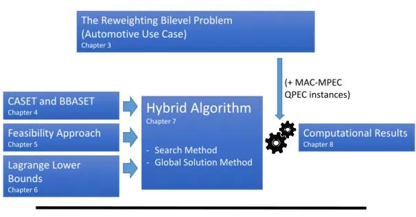
1.1. Chapter Overview . . . 4

2.1. MPEC Stationary Concepts (Example 2.1) . . . 14

3.1. Algorithmic Concept for the Reweighting Bilevel Problem . . . 45

4.1. Illustration of the CASET Algorithm . . . 47

4.2. Objective Function of (4.21) . . . 53

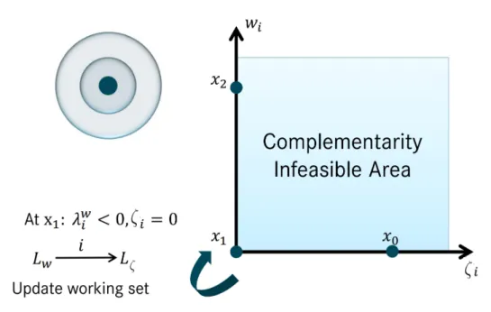
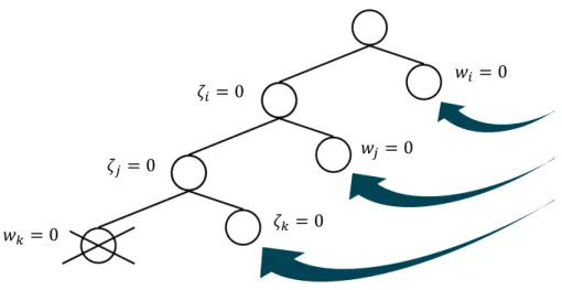
4.3. Illustration of the BBASET Algorithm for λζ_i, λζ_j, λw k ă0 . . . 55

6.1. Geometric Argument in Theorem 6.2 . . . 102

7.1. Recursive Algorithm Variant 1 . . . 114

7.4. Feasible Set of an Exemplary Reweighting Bilevel Problem with xPR2 . . . 122

7.5. Feasible Set of an Exemplary Reweighting Bilevel Problem with Two Connected Components for pXzpi`qq XPi` . . . 122

7.6. Simplified Diagram of Algorithm 14 . . . 130

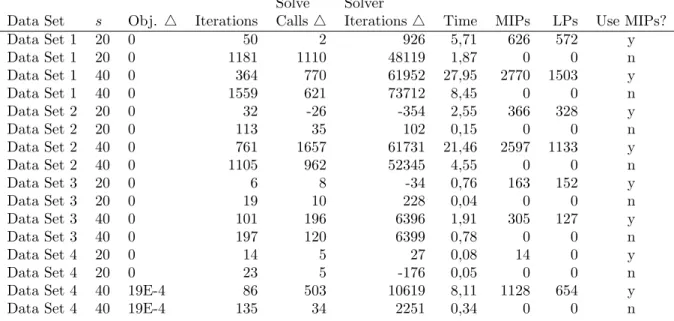
8.1. Hybrid Algorithm in Search Mode, qpec-100-1 (left), qpec-100-2 (right) . . . 160

(10)

List of Tables

3.1. Format Sample of the Technical Documentation . . . 25 3.2. A Randomized Data Sample . . . 31 5.1. Performance of Algorithm 8 on a small Test Set . . . 95 5.2. Performance of the Cplex MIQP Solver on the same Test Set . . 96 8.1. Objective Function Characteristics of the Reweighting Bilevel

Instances . . . 156 8.2. Characteristics of the QPEC Test Instances . . . 158 8.3. Computational Reference: l1 Elastic Interior Point Mehod . . . . 161 8.4. Computational Reference: Cplex 12.1 MIQP-Solver . . . 162 8.5. Performance Indicators . . . 162 8.6. Performance of Most Infeasible Branching by Repeated Calls to

the Cplex QP Solver . . . 163 8.7. Cplex MIQP Solver in Classic Branch-and-Bound Mode with

MIP-Starts provided by the Hybrid Algorithm in Search Mode . 164 8.8. Cplex MIQP Solver in Classic Branch-and-Bound Mode with

MIP-Starts provided by the Hybrid Algorithm in Search Mode . 164 8.9. Hybrid Algorithm compared to Cplex MIQP Solver on Global

Optima for the Reweighting Bilevel MPEC . . . 166 8.10. Hybrid Algorithm on the Reweighting Bilevel MPEC - Data Set 1 167 8.11. Upper Level Objective of the Lower Level Solution before and

after the Bilevel Optimization . . . 167 A.1. Iterations of the Hybrid Algorithm in Search Mode Part 1 on

QPEC Problems . . . 179 A.2. Iterations of the Hybrid Algorithm in Search Mode Part 2 on

QPEC Problems . . . 180

(11)

List of Tables xi

A.3. CPLEX MIQP Solver in Classic Branch-and-Bound Mode with

MIP-Starts provided by Hybrid Algorithm in Search Mode . . . 181 A.4. CPLEX MIQP Solver in Dynamic Search Mode with

MIP-Starts provided by the Hybrid Algorithm in Search Mode . 182 A.5. CPLEX MIQP Solver in Dynamic Search Mode with

MIP-Starts provided by the Hybrid Algorithm in Search Mode . 183 A.6. Data Set 2 -s “20: Hybrid Algorithm on the Proof of Global

Optimality . . . 185 A.7. Data Set 2 -s “50: Hybrid Algorithm on the Proof of Global

Optimality . . . 186 A.8. Data Set 3: Hybrid Algorithm on the Proof of Global Optimality 187 A.9. Data Set 4 -s “20: Hybrid Algorithm on the Proof of Global

Optimality . . . 188 A.10. Data Set 4 -s “40: Hybrid Algorithm on the Proof of Global

(12)

1. Introduction

In 2016 the Organization of Motor Vehicle Manufacturers (OICA) reported a pro-duction of over 94 million vehicles world wide, of which 60 million were passenger cars [73].

“Building 60 million vehicles requires the employment of about 9 million people directly in making the vehicles and the parts that go into them. This is over 5 percent of the world’s total manufacturing employment.”

– OICA [73] As one of the main contributors to the global economy, the automotive industry has been widely affected by the advances in digital technologies and the infor-mation revolution. Concepts in mobility and transportation are continuously evolving with the rise of new inventions. But it is not only the manufactured ve-hicle itself that has been influenced by such developments. As customer demands adjust to a world of e-commerce and digital retail, the area of product customiza-tion becomes more and more important [9]. In the context of a make-to-order manufacturing process, this leads to demanding challenges in terms of marketing and sales [38, 50, 67]. Against this backdrop, the availability of detailed demand forecasts has been shown to be of vital importance.

This research was inspired by a mathematical model for structural part demand forecasts, and its basis was provided by one of the global players in the premium automotive sector, the Mercedes-BenzR _{division of Daimler AG. The} mathemati-cal model is multicriterial [16] as it merges the information of historimathemati-cal customer orders and future demand forecasts. The solution to this problem is always uniquely determined, but it depends on a specific set of parameters.

The primary motivation behind this work is to investigate parameter settings of the forecast model that provide optimal results in a number of training

(13)

1.1. Introduction 2

ios. The question leads to a multilayered problem structure, which can then be formulated as a mathematical problem with equilibrium constraints (MPEC).

MPECs

MPECs have been an active field of research for several years [68, 74, 63, 33, 14]. Their origin in mathematical optimization goes back to researchers such as Cournot, Stackelberg and Nash, and they have been subject to research by many authors to this day.

Stackelberg introduces a problem for a market situation where two participants interact by deciding on individual strategies [69]. They are denoted as theleader

and thefollower. In their economical environment they supply the same type of product, forming the constellation of a duopoly. The key aspect in this model is that the leader can anticipate the decision of the follower, which is optimal in the follower’s corresponding perspective. This is an extension to the model of Cournot, which was introduced earlier and provides a foundation for the work of Stackelberg. In Cournot’s model both participants are equal and their decisions are both based on the best-answer principle. Stackelberg’s model entitles the leader to optimize his own profit by selecting a strategy according to the follower’s anticipated decision, and leads to a multilevel situation which is sometimes called a Stackelberg game.

As a breakthrough in Economics, Nash’s research on noncooperative games fol-lowed the results of Stackelberg’s publication. The Nash-Cournot equilibrium [58] denotes the situation where among several players that compete simultane-ously, none of them can increase their profit by a change of strategy under the assumption that all the other players will keep their selected strategy at the same time.

Hierarchical structures, as in the Stackelberg game, are the entry point to bilevel problems [15, 4]. In terms of mathematical optimization, this leads to the question of characterizing optimal points on the follower’s level. Common principles such as the Karush-Kuhn-Tucker conditions can be used under certain assumptions and lead to the element of equilibrium constraints.

(14)

1.1. Introduction 3

at a point xif

Gpxq ě0, Hpxq ě 0, GpxqHpxq “0. (1.1)

Within the scope of this work a number of solution techniques that are related to MPECs with linear complementarity constraints are investigated. The main achievement is the development of a hybrid solution algorithm and its application. Numerical experiments are conducted essentially with the data instances of the automotive industrial application, but also with data instances that are publicly available.

Structure of this Work

The final hybrid algorithm is a framework that connects different methodologies in a branch-and-bound environment. The theory behind the individual compo-nents will be introduced successively. The hybrid algorithm will be presented in its entirety in chapter 7.

In chapter 2 a range of common concepts that help to characterize stationary conditions for the feasible points of an MPEC is introduced and investigated [74, 49, 20, 62]. Difficulties for common solution algorithms are mentioned. These are due to the lack of stationary conditions, such as the Mangasarian-Fromovitz constraint qualification [22, 59] in MPECs. In this context the chapter will also develop proofs of two theorems that are known from related literature on the matter of B-stationarity, strong stationarity and the MPEC linear constraint qualification.

This is followed by the introduction of the parameter dependent demand forecast model with application to high complexity products, the so called reweighting problem. The model is a quadratic problem whose objective function matrix is positive semi-definite [59]. A new bilevel problem arises when the forecast model parameters are tuned with a data scenario that simulates a planning situation and evaluates the outcome. The bilevel problem is formulated as an MPEC whose feasible set is analyzed in its combinatorial structure. An investigation on the solution map of the lower level problem allows the possibility to prove the connectedness of the feasible area of the MPEC [47, 48, 13, 42].

(15)

1.1. Introduction 4

Stationary Concepts and Optimality Conditions for MPECs

Chapter 2

CASET and BBASET

Chapter 4 Feasibility Approach Chapter 5 Lagrange Lower Bounds Chapter 6

Hybrid Algorithm

Chapter 7 - Search Method

- Global Solution Method

Computational Results

Chapter 8

The Reweighting Bilevel Problem (Automotive Use Case)

Chapter 3

(+ MAC-MPEC QPEC instances)

Figure 1.1.: Chapter Overview

MPECs with linear complementarity constraints is reviewed. The method can be extended to find globally optimal solutions in the case of a convex objective func-tion with a branch-and-bound algorithm [34]. The chapter develops an extension to this approach for A-stationary points and shows how the CASET algorithm can be performed by solving a series of convex programs.

Another module of the hybrid algorithm is presented in chapter 5. An algo-rithm is reviewed that solves MPECs with linear objective function and linear complementarity constraints by a 0-1 integer based cut generation approach [24]. The method is analyzed and extended to a new adapted version that determines feasible areas in a general MPEC with linear complementarity constraints. Standard lower bounds in a branch-and-bound algorithm for MPECs, which are calculated with a relaxation of the complementarity constraints, can be inefficient [34, 14, 65, 28, 27]. Chapter 6 establishes a problem that yields a lower bound generated by the principles of weak duality. The resulting problem is also an MPEC but avoids some of the complexity by its absence of non-complementarity constraints. Under certain assumptions it holds that the objective function in this problem is convex. Furthermore a theorem is presented that characterizes unbounded directions of a convex function in the context of convex analysis [61].

(16)

1.1. Introduction 5

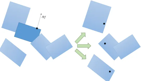
Chapter 7 presents the new hybrid algorithm that uses a combination of the previ-ously presented elements and investigates their interaction. The hybrid algorithm focuses on the solution of convex subproblems, and is divided into two stages. The first stage specializes in finding points with low objective value in an MPEC with convex objective function and linear complementarity constraints. For this search algorithm an abstract formulation is given that presents a geometrical generalization of the principle of the BBASET algorithm for feasible sets defined by a union of polytopes. The second stage specializes in proving global optimal-ity. Techniques are included that calculate constraints for the complementary variables and have proven to be effective in practice.

The last chapter concludes the investigation by a large number of computa-tional experiments. The commercial solvers CplexR _{and Gurobi}R _are imple-mented in a core unit for the solution of the various convex subproblems. A highly adjustable branch-and-bound framework with different parameter settings is wrapped around this core unit. The results of the hybrid solver are compared to the Cplex MIQP solver for instances of the reweighting bilevel MPEC, and are also compared to benchmarks of a related article for a number of instances that are publicly available [29]. They demonstrate that the hybrid algorithm shows viable performance in some instances. The subroutine that searches for a stationary point with low objective value performs well on the publicly available MPEC data. The solution of the bilevel problem in the training scenarios of the demand forecast model yields an increase of an average of 18% for the quality of the forecast.

(17)

2. Stationary Concepts and Solution Methods

for MPECs

We begin by introducing common stationary concepts and optimality conditions for general optimization problems, followed by specialized versions for the case of mathematical problems with equilibrium constraints (MPECs). The last section presents a list of references for a number of selected articles on the topic of solution methods and related results.

2.1. Common Stationary Conditions and Constraint

Qualifications

The most basic concepts of stationary conditions and constraint qualifications from general optimization are introduced briefly. One of the most valuable as-pects is the existence of multipliers at local optimal points, and in return the characterization of stationary points by the existence of multipliers. This princi-ple will be extended to the concept of MPECs in the next section.

A point is locally optimal if no descent is possible in the feasible part of an environment around this point, which is arbitrarily small. The characterization of feasible directions, which are considered around a feasible point, is achieved by introducing the tangent cone.

2.1 Definition (Tangent Cone, [22] def. 2.28, def. 2.31, [59] 12.2) The tangent cone of X at xPX is defined by

TXpxq:“ td | DpxkqkPNĎX, DptkqkPNP R, tk Ó0 : xk Ñx and pxk´xq{tkÑdu. (2.1)

If X is defined by continuously differentiable functions gi and hj as

X “ txP Rn | gipxq ď0, i“1, . . . , m, and hjpxq “0, j “1, . . . , ku, (2.2)

(18)

2.1. Common Stationary Conditions and Constraint Qualifications 7

then the linearized tangent cone at xPX is given by

Tlinpxq:“ td | ∇gipxqTdď0 @iP Ipxq and ∇hjpxqTd“0u. (2.3) We notice that the definition of the linearized tangent cone is possibly easier to manage than the general definition. Since problems with linear constraints are of major importance in optimization, it is often adequate to work with the linearized tangent cone. The equality of both tangent cones is implied by so called constraint qualifications.

We note that_Tpxq ĎTlinpxqalways holds [22, section 2.2]. In this section, if not

stated otherwise, let X be defined as in (2.2).

2.2 Definition (Abadie-CQ, [22] def. 2.33) The Abadie constraint qualifi-cation (Abadie-CQ) is satisfied at xPX if

Tpxq “Tlinpxq. (2.4)

2.3 Definition (KKT-point, [22] def. 2.35) Letf be a continuously differ-entiable function. A point x˚ _{is called KKT-point (Karush-Kuhn-Tucker-point)}

of the problem

min x fpxq xP X

(2.5)

if it satisfies the KKT-conditions: There exist multipliersλ “ pλg, λhq such that

0“∇fpx˚q ` m ÿ i“1 λg_igipx˚q ` k ÿ j“1 λhj∇hjpx˚q hpx˚q “0 λg ě0, gpx˚q ď0, λgTgpx˚q “0. (2.6)

2.1 Theorem (Dual Multiplier Existence, [22] Prop. 2.36)

If x˚ _{is a local optimum of problem (2.5) where} _f _{is continuously differentiable}

and the Abadie-CQ holds atx˚ _{then there exist dual multipliers} _λ

“ pλg, λhq as

(19)

2.1. Common Stationary Conditions and Constraint Qualifications 8

Under certain conditions the existence of dual multipliers can be linked back to the local optimality of the corresponding point. In the case of a convex program it holds that the KKT-conditions provide a sufficient condition for optimality.

2.4 Definition (Convex Problem, [22] 2.2.4) Problem (2.5) is called con-vex if f and gi, i “ 1, . . . , m, are continuously differentiable and convex, and if hj, j “1, . . . , k, are affine linear.

It holds that every locally optimal point of a convex problem is also globally optimal [22, lemma 2.43].

2.2 Theorem ([22] Prop. 2.46)

Ifx˚ _{is a KKT-point of (2.5) and (2.5) is convex, then} _x˚ _{is optimal.}

We recall that the existence of KKT-multipliers requires the Abadie-CQ. There are two common constraint qualifications that imply the Abadie-CQ and are more applicable.

LetIpxq be the set of indices of the active inequality constraints

Ipxq “ ti| gipxq “ 0u. (2.7)

2.5 Definition (MFCQ, [22] def. 2.38) The Mangasarian-Fromovitz constraint qualification (MFCQ) is satisfied at xPX if

1. the gradients _∇hjpxq for j “1, . . . , k are linearly independent and

2. there exists d P Rn such that ∇gipxqTd ă 0, @i P Ipxq and ∇hjpxqTd “ 0, @j “1, . . . , k.

The MFCQ ensures that the feasible set is nonempty which naturally is an im-portant aspect of interior point algorithms.

2.6 Definition (LICQ, [22] def. 2.40) The linear independence constraint qualification (LICQ) is satisfied atxP Xif the active constraint gradients∇gipxq, iP Ipxq and ∇hjpxq are linearly independent.

2.3 Theorem ([22] prop. 2.39, 2.41)

The following relations between the constraint qualifications hold:

(20)

2.2. Stationary Concepts for MPECs 9

2.2. Stationary Concepts for MPECs

We introduce the general mathematical problem with equilibrium constraints (MPEC)

minfpxq

gpxq ď 0, hpxq “ 0

Gpxq ě 0, Hpxq ě0, GpxqTHpxq “0

(2.9)

wheref :Rn_Ñ_R_,_g _:_Rn _Ñ_Rk_,_h_:_Rn_Ñ_Rl_,_{G, H} _:_Rn_Ñ_Rm_{are differentiable} functions.

For the characterization of a local optimal solution the concept of B-stationarity is introduced. Varying definitions in different articles can be found (as shown below), for further considerations the following definition is used:

2.7 Definition (B-stationary, [74] def. 2.2) A feasible pointxof an MPEC (2.9) is said to be B-stationary (Boulingard-stationary) if

∇fpxqTdě0 @dPTpxq. (2.10)

Remark 2.1

1. Iff is continuously differentiable, then every local optimum is B-stationary [22, lemma 2.30].

2. The opposite of point 1 is generally not true which can be seen by consid-ering a local maximum x with ∇fpxq “0 (in a minimization problem).

3. The points 1 and 2 still hold if no complementarity constraints are present (m “0).

Remark 2.2 Other definitions of B-stationarity found in related articles use the linearizations of the constraint functions [20, def. 3.2][62, def. 2.1]. Let x be a feasible point of the MPEC (2.9), x is denoted B-stationary in definition 2.1 of [62], if d“0 is optimal in

(21)

2.2. Stationary Concepts for MPECs 10 min d ∇fpxq T_d gpxq `∇gpxqTdď0 hpxq `∇hpxqTd“0 0ďGpxq `∇GpxqTd K Hpxq `∇HpxqTdě0. (2.11)

(Where the operatorxKyfor two vectorsxandyindicates that the scalar product

xT_y “0.)

However, with this definition the following example is mentioned: Let the corre-sponding functionsf,G and H of the MPEC (2.9) and system (2.11) be defined as in

minfpx, yq:“ px´1q2` py´1q2

0ďGpx, yq:“xK Hpx, yq:“yě0.

(2.12) We note thatx“ p1,0q is a local optimum. And as we are going to see, it is also

strongly stationary (def. 2.10). But ˆd“ p´1,1qis feasible in (2.11) and indicates

that the objective value is negative.

∇fp1,0qTdˆ“ p0,´2qp´1,1qT “ ´2 (2.13)

It follows that x is not B-stationary in the sense of (2.11) which might not have been the intention of the authors of [62]. An e-mail concerning this topic remained unanswered.

A more suitable way to introduce B-stationarity with linearized constraint func-tions is the following condition

0“min∇fpxqTd

dPT_{M P EC}lin pxq

(2.14) whered lies in the MPEC linearized tangent cone which will be introduced next (def. 2.8).

For this and for many further aspects, we introduce the following index sets for any feasible point xof the MPEC (2.9):

(22)

2.2. Stationary Concepts for MPECs 11 Ig :“ ti | gipxq “ 0, iP t1, . . . , kuu I`0 :“ ti | Gipxq ą 0, Hipxq “0, iP t1, . . . , muu I0` :“ ti | Gipxq “ 0, Hipxq ą0, iP t1, . . . , muu I00 :“ ti |Gipxq “ 0, Hipxq “0, iP t1, . . . , muu. (2.15)

The definitions depend on the specific pointx and are defined in this sense if no further argument is present. Now we introduce the MPEC version of the Abadie-CQ with a definition of the linearized tangent cone specialized for MPECs.

2.8 Definition (MPEC Abadie-CQ, [74] def. 3.1) Letxbe a feasible point for the MPEC (2.9). The MPEC-Abadie-CQ is satisfied at x if

Tpxq “T_{M P EC}lin pxq (2.16) where Tlin M P EC :“ td PRn such that: ∇gipxqTdď0, @iPIg ∇hipxqTd“0, i“1, . . . , l ∇GipxqTd“0, @iP I0` ∇HipxqTd“0, @iPI`0 ∇GipxqTdě0, @iPI00 ∇HipxqTdě0, @iPI00 p∇GipxqTdqp∇HipxqTdq “0, @iPI00u. (2.17) Remark 2.3

• The definition of B-stationarity (def. 2.7) is equivalent to the alternative definition of (2.14) if we assume that the MPEC-Abadie-CQ holds.

• It always holds that Tpxq ĎT_{M P EC}lin pxq[74].

• The difference between the MPEC linearized tangent cone Tlin

M P EC and the general linearized tangent cone _Tlin _{at a point} _x _{of the MPEC (2.9) is the} last block of constraints

(23)

Thus the MPEC version of the linearized tangent cone is more restrictive than the general version.

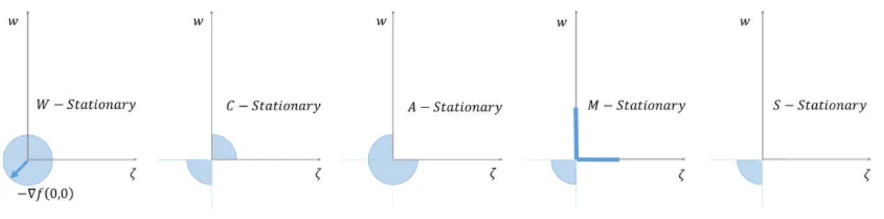
Working with the tangent cone is often impractical. Other stationary concepts use formulations with dual multipliers in the same fashion as the KKT-conditions. The following definitions are closely related to each other. It is, as Leyffer and Munson wrote in [49], “the alphabet soup of MPEC stationarity”.

2.9 Definition (W-stationary, [49] def. 2.1, [74] def. 2.3) A feasible point

xof the MPEC (2.9) is said to be W-stationary (weakly stationary) if there exist multipliers λ“ pλg, λh, λG, λHq PRk`l`2m, such that:

0“∇fpxq ` ÿ iPIg λg_i_∇gipxq ` l ÿ i“1 λh_i_∇hipxq ´ m ÿ i“1 pλG_i ∇Gipxq `λHi ∇Hipxqq λg_Ig ě0, λG_I`₀ “0, λH_I₀_` “0. (2.19) The definition of W-stationarity is equivalent to the KKT-conditions of the so calledtightened MPEC (TMPEC) at x:

min x1 fpx 1 q gpx1q ď 0, hpx1q “ 0 GI0`YI00px 1 q “0, HI`0YI00px 1 q “0. (2.20)

We recall that the setsI`0, I0` and I00 in (2.15) depend on x.

2.10 Definition (C-, A-, M-, S-stationary) ([49] def. 2.2, [74] def. 2.4 - 2.7, [20] def. 3.3)

Let x be weakly stationary and let there exist multipliers as in (2.19):

• x is C-stationary (Clarke-stationary) if λG

i λHi ě0 for all iPI00. • x is A-stationary (alternatively stationary) if λG

i ě 0 or λHi ě 0 for all iP I00.

• x is M-stationary (Mordukhovich-stationary) if either λG

i ą0or λHi ą0 or λG

i λHi “0 for all iP I00.

• x is S-stationary (strongly stationary) if λG

(24)

The stationary concepts satisfy the following chains of inclusion [74, 49]:

pS´Stationaryq ó pM ´Stationaryq ó ó pA´Stationaryq pC´Stationaryq ó ó pW ´Stationaryq (2.21)

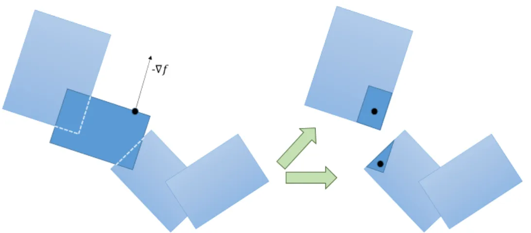
Example 2.1 The different concepts of stationarity are illustrated on an MPEC with a single constraint for two non-negative complementary variables.

min

w,ζPRfpw, ζq

w, ζ ě0

wζ “0

(2.22)

The index sets at p0,0q are

I`0 “I0` “ H, I00 “ t1u. (2.23)

Figure 2.1 illustrates the possible directions of the negative gradient ´∇fp0,0q

that correspond to the individual MPEC stationary concepts. This means that if the negative gradient lies in the indicated set of directions (blue) then the corre-sponding stationary definition is satisfied at p0,0q.

2.4 Theorem

Letxbe a feasible point of the MPEC (2.9) and assume that the MPEC-Abadie-CQ is satisfied atx.

1. If x is strongly stationary then x is B-stationary [74].

2. If f, g, h,G and H are continuously differentiable andx is locally optimal then x is M-stationary [74].

(25)

− − − − −

−∇ 0,0

Figure 2.1.: MPEC Stationary Concepts (Example 2.1)

Proof 1) Since the MPEC-Abadie-CQ is satisfied at x, we can use (2.14) to

characterize B-stationarity: d “0 solves

min∇fpxqTd

dPT_{M P EC}lin pxq.

(2.24)

By the definition of a strongly stationary point (def. 2.10) it follows that there exist multipliers λ as in (2.19) with λG

i ě 0 and λHi ě 0 for all i P I00. With dPT_{M P EC}lin the following three cases may appear:

1. If iPI`0 it follows that ∇HipxqTd“0 and from (2.19) λGi “0. 2. If iPI0` it follows that ∇GipxqTd“0 and from (2.19) λHi “0.

3. If iPI00 it follows that ∇GipxqTdě0 and ∇HipxqTdě0 and from strong stationarity that λG

i , λHi ě0.

Thus for any elementdPTM P EClin pxqit follows that

´∇fpxqTd“ p ÿ iPIg λg_i_∇gipxq ` l ÿ i“1 λh_i_∇hipxq ´ m ÿ i“1 pλGi ∇Gipxq `λHi HipxqqqTd “ ÿ iPIg λg_i loomoon ě0 ∇gipxqTd loooomoooon ď0 ` l ÿ i“1 λh_i _∇hipxqTd loooomoooon “0 ´ ÿ iPI`0 p λG_i loomoon “0 ∇GipxqTd`λHi ∇HipxqTd loooomoooon “0 q ´ ÿ iPI0` pλGi ∇GipxqTd loooomoooon “0 ` λHi loomoon “0 ∇HipxqTdq ´ ÿ iPI00 p λG_i loomoon ě0 ∇GipxqTd loooomoooon ě0 ` λH_i loomoon ě0 ∇HipxqTd loooomoooon ě0 q ď0. (2.25)

(26)

This shows thatx is B-stationary.

2)The proof for this point is not presented in detail here. For more information the reader is referred to the related article [74] instead. The following is a brief outline: First it can be shown that for affine linear functionsg,h,GandHit holds that any local solution x is M-stationary. In order to show this, the existence of Fritz-John type multipliers is utilized. These always exist if the functions of an optimization problem are continuously differentiable [74, thm. 2.1]. For further information on Fritz-John multipliers see [22] section 2.2.5. Since the MPEC-Abadie-CQ is satisfied, the case of affine linear constraint functions is sufficient. The complete proof can be found in [74] theorem 3.1.

3) The following example shows a B-stationary point that is not strongly sta-tionary: min w,ζPR´w´ζ wζ “0 w, ζ ě0 pζ´wqpζ`wq “ 0 ζ´wě0 ζ`wě0 (2.26)

The only feasible point of this system is p0,0q which is obviously B-stationary.

Regarding the strong stationary condition, this would require positive multipliers λ“ pλ1, λ2, λ3, λ4q ě 0 such that 0“ ˜ ´1 ´1 ¸ ´λ1 ˜ 1 0 ¸ ´λ2 ˜ 0 1 ¸ ´λ3 ˜ ´1 1 ¸ ´λ4 ˜ 1 1 ¸ . (2.27) The second of both components reveals that this equation cannot be satisfied for λě0 and thus p0,0q is not strongly stationary.

From point 3 of theorem 2.4 we see that the strong stationary condition is more restrictive than what is needed for local optimality. On the other hand all the weaker stationary concepts (W-, A-, C- and M-stationary) allow first order de-scent directions. This can be seen with the following example [49, 2.7]:

(27)

minpw´1q2`ζ3`ζ2 subject to 0ďw Kζ ě0. (2.28)

The point p0,0q is A- and M-stationary, but moving along the x-axis provides a

feasible descent direction.

The following condition allows to achieve equality of B- and strong stationarity under the MPEC-Abadie-CQ.

2.11 Definition (MPEC-LICQ, [74] def. 2.8, [20] def. 3.1) Letxbe a fea-sible point of the MPEC (2.9). The MPEC-LICQ (MPEC linear independence constraint qualification) is satisfied atxif the following active constraint gradients are linearly independent:

t∇gipxq | iPIgu Y t∇hipxq | i“1, . . . , lu Yt∇Gipxq | iPI0`YI00u Y t∇Hipxq | iPI`0 YI00u

(2.29)

2.5 Theorem ([20] lem. 4.3)

Let x be a feasible point of the MPEC (2.9) and let the MPEC-Abadie-CQ be satisfied at x. If the MPEC-LICQ is satisfied at x and x is B-stationary, then x is also strongly stationary .

Proof From the MPEC-Abadie-CQ and B-stationarity we conclude that (2.14)

holds: d“0 solves

min_∇fpxqTd

dPTM P EClin pxq.

(2.30) We take a look at the condition

p∇GipxqTdqp∇HipxqTdq “0, @iPI00 (2.31) from the definition of the MPEC linearized tangent cone (2.17). LetI1 andI2 be a disjunct partitioning of the setI00

I1YI2 “I00

I1XI2 “ H.

(28)

Let _TpI1, I2q Ď T_{M P EC}lin pxq be the subset of the MPEC linearized tangent cone

where the constraint (2.31) is exchanged for a number of more restrictive linear constraints:

TpI1, I2q:“ tdPRn such that: ∇gipxqTdď0, @iP Ig ∇hipxqTd “0, i“1, . . . , l ∇GipxqTd“0, @iPI0` ∇HipxqTd“0, @iPI`0 ∇GipxqTdě0, @iPI00zI1 ∇HipxqTdě0, @iPI00zI2 ∇GipxqTd“0, @iPI1 ∇HipxqTd“0, @iPI2u. (2.33)

It follows that for each such partitioning pI1, I2q the vector d “ 0 is always an

optimal solution of the problem

min_∇fpxqTd

dPTpI1, I2q.

(2.34) This is due to the fact that d “ 0 is always feasible and by the B-stationary

condition no solution with lower objective value can exist.

We notice that problem (2.34) is a pure LP, thus we can conclude that the KKT-conditions are satisfied at d“0 and the following multipliersλ exist

0“∇fpxq ` ÿ iPIg λg_i_∇gipxq ` l ÿ i“1 λh_i_∇hipxq ´ m ÿ i“1 pλG_i ∇Gipxq `λHi ∇Hipxqq λg_Ig ě0 (2.35) but with the following restrictions, depending on pI1, I2q

• for i P I2 there are active inequality constraints ∇GipxqTd ě 0 in the definition of _TpI1, I2q. It follows thatλG_I₂ ě0;

(29)

• for i P I1 there are active inequality constraints ∇HipxqTd ě 0 in the definition of TpI1, I2q. It follows thatλH_I₁ ě0;

• for iP I`0 there are no constraints present for ∇GipxqTd in TpI1, I2q thus it follows that λG

I`0 “0;

• for iP I0` there are no constraints present for ∇HipxqTd in TpI1, I2q thus it follows that λH

I0` “0.

With the MPEC-LICQ it follows that the multipliers of (2.35) are unique. Thus for any partitioningpI1, I2qwe will receive the same multipliers.

SinceλG_I₂ ě0 andλH_I₁ ě0 for each partitioning it follows thatλG, λH ě0, @iPI00.

This concludes that the multipliers λ satisfy the requirements of definition 2.10

which shows thatx is strongly stationary.

Similar to the MPEC-LICQ there also exists an MPEC-MFCQ.

2.12 Definition (MPEC-MFCQ, [62] Def. 2.5) The MPEC-MFCQ is sat-isfied at a feasible point x of the MPEC (2.9) if there exists a non-zero vector

dPRn such that ∇GipxqTd“0, @iP I0` ∇HipxqTd“0, @iPI`0 ∇hipxqTd“0, i“1, . . . , l ∇gipxqTdą0, @iPIg ∇GipxqTdą0, @iPI00 ∇HipxqTdą0, @iPI00 (2.36)

and the vectors of the following set are linearly independent

t∇Gipxq | iPI0`u Y t∇Hipxq | iPI`0u Y t∇hipxq | i“1, . . . , lu. (2.37) We want to provide an example that explains why solving MPECs poses potential difficulties. First we note that the standard MFCQ (def. 2.5) does not hold at any point of the MPEC, since the gradients of the constraints

(30)

Gipxq ě 0, Hipxq ě 0, GipxqHipxq ď 0, @i“1, . . . , m (2.38) at a feasible pointxare always linearly dependent with some positive multipliers. But for various applications the MFCQ provides existence of KKT multipliers, since it implies the Abadie-CQ. This is crucial for many non-linear solution meth-ods.

The end of this section presents a helpful result which yields that an M-stationary point is locally optimal under certain conditions without requiring the MPEC-Abadie-CQ. For this we need two weaker forms of convexity:

2.13 Definition (Pseudo- and Quasiconvex, [52])

A differentiable function f :X ÑR is called pseudoconvex if for x, y P X

∇fpxqpy´xq ě0ñfpyq ě fpxq. (2.39)

A differentiable function f is called quasiconvex if

fpλx` p1´λqyq ďmaxtfpxq, fpyqu, @x, y P X. (2.40)

2.6 Theorem (Sufficient M-stationary condition, [74] Thm. 2.3)

Let x be an M-stationary point of the MPEC (2.9), i.e. there exist multipliers such that 0“∇fpxq ` ÿ iPIg λg_i∇gipxq ` l ÿ i“1 λh_i∇hipxq ´ m ÿ i“1 pλG_i ∇Gipxq `λHi ∇Hipxqq λg_Ig ě0, λG_I`₀ “0, λH_I₀_` “0 either λGi ą0, λHi ą0 or λGi λHi “0, @iPI00. (2.41)

(31)

Letf be pseudoconvex at xand the following functions be quasiconvex: gi for i P Ig, hi for i P IJ`, ´hi for i P J´, Gi for i P I0´` YI

´ 00H, ´Gi for iPI₀`_`YI₀₀`_H YI₀₀`,Hi for iPI`´0YI00´G, ´Hi for iPI``0YI00`GYI00`. 1. IfI´ 0`YI ´ `0YI00´GYI ´

00H “ Hit follows thatxis a globally optimal solution of the MPEC.

2. If either I´

00GYI00´H “ H or for all feasible x1 in a sufficiently small set around x it holds that

Gipx1q “ 0, Hipx1q “0, @iPI00´GYI00´H (2.43) then x is a locally optimal solution of the MPEC.

The proof of this theorem can be found in [74], theorem 2.3.

With this result it is easy to derive optimality criteria for the case where the constraint functions are affine linear and the objective function is convex. This class of MPECs will be investigated in detail in the subsequent chapters.

Corollary 2.1

Letx be a feasible point of MPEC (2.9) and assume that f is convex and g, h, Gand H are affine linear.

1. If x is strongly stationary then x is locally optimal. 2. If x is strongly stationary and λG

I0` ě 0 and λ H

I`0 ě 0 then x is globally optimal.

(32)

2.3. Solution Algorithms for MPECs 21

Proof 1) From strong stationarity follows M-stationarity and I´

00G “I00´H “ H. The result follows with point 2 of theorem 2.6.

2) It further holds that

I´ 0` “ H ôλ G I0` ě0 (2.44) I´ `0 “ H ôλHI`0 ě0. (2.45)

And sincex is strongly stationary it follows that

I´

00GYI

´

00H “ H. (2.46)

The result follows with point 1 of theorem 2.6.

2.3. Solution Algorithms for MPECs

This section provides a small number of selected references to solution methods and related articles for MPECs. Among them are algorithms, such as interior point methods or regularization schemes, that will not be discussed in detail within the extent of this work. The references are mainly in chronological order, ending with three monographs that have a summarizing character.

In [51] Luo et al. present applications of PSQP (piece wise sequential quadratic programming) methods to MPECs. Their results include local convergence under the MPEC-LICQ.

In [64] Scholtes investigates a regularization scheme for MPECs as (2.9). The regularization is based on:

minfpxq

gpxq ď 0, hpxq “ 0

Gpxq ě0, Hpxq ě0, GpxqiHpxqi ďt, i“1, . . . , m

(2.47)

for a non-negative scalar t. He shows that under suitable assumptions a series of stationary points of systems (2.47) converges to a C-stationary point of the MPEC. The monograph [62] by Ralph and Wright establishes more properties on algorithms with this regularization scheme. Another regularization scheme is the Lin-Fukushima approach, as referenced below.

(33)

2.3. Solution Algorithms for MPECs 22

In [75] Zhang et al. present an algorithm that solves MPECs with convex ob-jective function and affine linear complementarity constraints. The algorithm investigates extreme points and directions around the current point of iteration. These extreme elements determine a face of the feasible area around this cur-rent point. The SQP step is then carried out on this face. At termination the algorithm yields a locally optimal point.

In the monograph [60], Demiguel et al. present an interior point method for relaxations of the following type.

The MPEC in [60] is defined as min

x fpxq hpxq “0

0ďGpxq K Hpxq ě 0.

(2.48)

The relaxation forpδ1, δ2, δ3q ě 0 is min px,w,ζ,sqfpxq hpxq “ 0 Gpxq ´w“0 Hpxq ´ζ “0 s1´w“δ1 s2´ζ “δ2 s3`wTζ “δ3 w, ζ, sě0. (2.49)

where the parameters δ1, δ2 and δ3 gradually decrease in their algorithm. The vector s allows the possibility to rewrite the system with equality constraints. Their article also holds a useful collection of references in the introduction. In [25] Hu and Ralph investigate the application of penalty methods to MPECs. In the monograph [20], Fletcher et al. investigate the local convergence of SQP methods. Their article is helpful in understanding the difficulties with linear de-pendent active constraints in MPEC solution methods. They achieve superlinear convergence around a strongly stationary point under a number of reasonable assumptions.

The monograph [49], by Leyffer and Munson, presents a globally convergent filter method. In an iteration cycle, a linear problem is used to estimate the active constraint set of the solution, then a QP with equality constraints is solved. By applying a filter they achieve convergence to a B-stationary point of the MPEC.

(34)

2.4. Outlook 23

In [2] Audet et al. investigate reformulations of linear 0-1 mixed integer program-ming problems to MPECs with linear objective function and linear complemen-tarity constraints. They present the equivalent versions of cuts, such as e.g. the common Gomory cuts from mixed integer programming, as well as branch-and-cut strategies in the MPEC world. In relation to this, the monograph [55], by Mitchell et al., focuses on tighter relaxations of MPECs.

In the monograph [37], Kanzow et al. show that the Lin-Fukushima-regularization can create a series of NLPs whose stationary points converge to a C-stationary point of the MPEC (2.9). For this, the complementarity constraints are replaced by

pGipxq `tqpHipxq `tq ´t2 ě0, i“1, . . . m GipxqHipxq ´t2 ď0, i“1, . . . , m

(2.50) for a non-negative scalart that decreases during the algorithm.

In [30], J´udice gives an overview of algorithms for MPECs with linear objective function and linear complementarity constraints. An extensive bibliography on bilevel programming and MPECs can be found in [68] by Dempe. The monograph [31] by J´udice contains a collection of solution techniques for MPECs with linear complementarity constraints.

2.4. Outlook

The following chapter changes from the theoretical background of MPECs to a practical quadratic problem that has its origin in an application related to the automotive industry. After an introduction to the problem and some further investigations on the matter of the solution map of quadric problems, the topic of MPECs returns in section 3.4. In this section a bilevel problem is introduced that can be formulated with the element of linear equilibrium constraints.

(35)

3. The Reweighting Problem

The automotive industry provides a good example of so called high complexity products [50, 38, 67]. In this chapter a problem with complementarity con-straints, which originates from a demand forecast model for multivariant product configurations, is presented.

“Mass customization has been viewed as desirable but difficult to achieve in the volume automotive sector.”

– Production and Operations Management [9] Visiting the online configurator of a leading automotive manufacturer in the premium segment provides a good impression on the topic [72]. The customer’s choice depends not only on the specific model series, color and engine but is extended to a large number of optional equipment ranging from interior design to advanced driving assistance systems.

A complete customer order of a Mercedes-BenzR _{vehicle holds the information} of a binary vector with hundreds of entries. It is considered highly likely that the daily output of a single factory does not contain two identical vehicles.

Beyond what the customer can see lies a large rule-based documentation. This translates the customer configuration into the technical information that is needed to produce the vehicle in full detail (see [38] for additional information). The documentation especially holds the list of all structural elements. Figure 3.1 shows a sample of the data format. Each row represents a technical part in combination with its physical position that might possibly be present in the final product. Whether or not it is present depends on the evaluation of a potentially lengthy Boolean expression (column “Rule” in table 3.1). The variables of this expression are (without further detail) the binary specifications of the customer order. The fully translated vehicle holds the information of a binary vector with about 10,000 entries, or a floating point vector with thousands of entries, if the

(36)

3.1. The Reweighting Problem 25

Technical Part Position Description Rule A188780201 100-100.1 _{Park Distance Control}Distance Ring 189;

A188733208 120-120.1 Pipe Cover Brushed

(686^588)^ (123 ^ 543 ^ 555

^678 _546)^ (686^588); A178669405 120-120.2 Pipe Cover

Black (123^ 543 ^ 555^678_546)^ (686^588); A199725507 250-250.15 Combined Instrument: Odometer, Oil-Pressure Control, White Backlight (R272^766 ^434 _344 ^665 ^455 _915) ^ (566^777) ^ (458_669_155) ^ (532_343) ^546_R32; Table 3.1.: Format Sample of the Technical Documentation

demands for technical parts of the same type are accumulated. These entries are denoted shortly as parts.

The increasing variety presents a challenge in acquiring detailed demand forecasts. Considering the data of optional equipment selection in the layer of information that is visible to the customer, we see that this layer holds aspects which are observable for marketing and sales. However, extending the analysis and predic-tion of customer and market behavior to the layer of parts and their demand is difficult.

In the following section we present a given demand forecast model that is applica-ble to any high complexity product. The model is based on a convex optimization problem with a multicriterial objective function, and depends on a set of param-eters which are related to a certain prognosis input: We assume that a sales or marketing department (or some other source) provides a certain prognosis for some of the optional equipment specifications in a future demand period. The model connects this option planning input with the knowledge about historical product configurations that hold information of customer behavior and previous part demands.

The final step is to train this model with data scenarios that simulate the situ-ation of a demand forecast requirement. The result of the forecast can then be compared to the desired demand outcome and thus be evaluated. This, let us call

(37)

3.2. The Demand Forecast Model 26

it training phase, is conducted by solving a bilevel problem. The bilevel problem can then be formulated as an MPEC and is subject to the solution techniques that will be developed within the scope of this work.

3.2. The Demand Forecast Model

The demand forecast model is constructed in three steps. It is based on a param-eter dependent convex optimization problem, and we focus on the aspects related to its application.

1) Historical Data and a Vector based Representation

We assume that a set of product configurations exists that are suitable as a foundation for the current demand forecast scenario. These might e.g. be con-figurations of the same model series, or concon-figurations that have been ordered in the same market segment as the one that is currently of interest. Let us assume that these historical orders ortemplates are given by a finite nonempty set

th˜i | iPIHistu ĂRm. (3.1) Next we introduce corresponding planning orders ˜xi _P _Rn˜_,_i_P_I

Hist, that resemble the outcome of the demand prognosis. For each of the historical orders we define a feasible area around it. This feasible area contains the planning order and is denoted bypp˜hiq. A few examples of how pp˜hiq might look like are

1. ˜ xi P pp˜hiq “ B}¨}1p˜h i_, iq “ txP Rm | m ÿ j“1 |xj ´˜hij| ăiu for given constantsi ą0;

(3.2) 2. ˜ xi Ppp˜hiq “ txP Rm| x“ri˜hi, ri ě0u; (3.3) 3. ˜ xi Ppp˜hiq “ txP Rm|x“ri˜hi, rmin ďri ďrmaxu for given constants rmin ă1ărmax.

(38)

The solution of the final optimization problem will yield optimal values ˜x˚i _and represent the result of the prognosis. At this point we make the following assump-tion: We assume that the parts demand of a single given order can be presented as a real vector inRp_{, for some} _p_P_N_{. We further assume that a function exists}

˜

T :Rm ÞÑRp (3.5)

that maps a planning order ˜xi _{to its resulting parts demand.}

Additional restrictions regarding the entirety of all planning orders can be intro-duced. We give two examples that extend (3.2) and (3.3) respectively:

1. x˜i Ppph˜iq “B}¨}1ph˜ i_, iq, @iPIHist ÿ iPIHist i ďtotal (3.6)

for a given number total ą0, or for the second point

2. x˜i Ppp˜hiq “ txP Rm|x“ri˜hi, rmin ďri ďrmaxu, @iP IHist

ÿ

iPIHist

ri “c. (3.7)

for a given constant cą0. The first alternative (3.6) allows the planning order

to differ from the historical template ˜hi_{, but the sum over all these differences is} bounded. In the second example (3.7) the planning order ˜xi _{is a scaled version} of the historical template but the total sum of these scaling factors is fixed. Further, we assume that the restrictions on the planning orders can be modeled by a set of linear constraints with positive decision variables. If required, we introduce additional variables such as for the elementsri in (3.7).

We denote the resulting linear system with positive decision variables as

Hx“h, xě0 (3.8)

where H P Rkˆn and h P Rk are constant and x P Rn. We continue with the

following requirements

(39)

We see that the first step in the modeling process is highly flexible. Each of the given alternatives can be translated to a certain meaning in terms of the manufacturer. Which approach is most suitable for the given situation depends on the specific data, as well as on the expectations of the user.

2) Deviation of Planning and History

One intention behind this modeling concept is to preserve the information that is contained in the vectors ˜hi, i P IHist since it represents customer behavior. We introduce a term that penalizes the deviation of the planning order from the historical template. This term is then added to the objective function of the model. A suitable example would be

min ˜ xi_: _i_P_IHist n ÿ j“1 px˜i_j´˜hi_jq2. (3.9)

If we reconsider example (3.7) then (3.9) is equivalent to min ˜ xi_{: ı}_P_I Hist ÿ iPIHist pri´1q2. _(3.10)

To this point we notice that the optimization of the model penalizes the deviation from the historical templates, and the historical templates are feasible at the same time. Thus the model, in the current state, should simply return the historical templates ˜x˚i _“_h˜i_{as a result. We continue with the last step where the objective} function becomes multicriterial.

3) Option Planning Rates

In the last step we want the model to reflect the option planning input that is given beforehand. The option planning input reflects changes in the market segment (or current planning area) on the level of option take rates. We assume that this input is presented by a real vector b “ pb1, . . . , bmq that correspond to the entries in the vector representation of both the historical data ˜hi and the planning output ˜xi_, _i

PIHist.

A prognosticated rate of bj0 for the component with index j0, is met if

ř

iPIHistx˜ij0 cardpIHistq

(40)

wherecarddenotes the cardinality of the set. It is also possible to determine the historical option take rates

bHist_j :“ ř

iPIHist˜hij cardpIHistq

, j P IHist (3.12)

which supposedly differ from the new option planning b.

We add a term to the objective function which penalizes the deviation of input rates and outcome. The term is given by

m ÿ j“1 γj| ř iPIHistx˜ i j cardpIHistq ´bj| (3.13)

and depends on a positive parameter vector γ P Rm_ě₀ that represents a

prioriti-zation of the individual option planning rates. The complete objective function is min ˜ xi_: _i_P_IHist ÿ iPIHist m ÿ j“1 px˜i_j´˜hi_jq2` m ÿ j“1 γj| ř iPIHistx˜ij cardpIHistq ´bj|. (3.14) Now as a last step we use the representation of (3.8) and rewrite the objective function in a more general format. The deviation of the take rates (3.13) is then represented by a parameterized function f₂γ in the final model, the deviation of planning and historical orders (3.9) is represented by a functionf1. The demand prognosis model is min x f1pxq `f2pxq Hx“h xě0 f1pxq:“xTQx`cTx f₂γpxq:“ m ÿ j“1 γj|pAx´bqj|. (3.15)

where we assume thatQ PRnˆn is a symmetric positive-definite matrix, cP Rn,

H P Rkˆn, h P Rk, A P Rmˆn and b P Rm. We introduce additional slack and

(41)

3.2. The Demand Forecast Model 30 min px,u,vqx T_Qx `cTx` m ÿ j“1 γjpuj `vjq Hx“h Ax`u´v “b x, u, v ě0. (3.16)

3.1 Definition (Reweighting Problem) The problem given by (3.16) is de-noted the reweighting problem.

The term reweighting is related to the special case of the modeling approach (3.7) where every planning order is a reweighted version of the corresponding historical template. (See example 3.1 below.)

We have assumed the existence of a function ˜T that maps a planning order ˜xi to its parts demand in (3.5). We now assume that we can find an equivalent function

T :Rn ÞÑRp (3.17)

that maps a given vectorx(that represents all planning orders) to the aggregated parts demand. This means for a solutionx˚ _{of (3.16) it holds}

Tpx˚q “ ÿ iPIHist

˜

Tpx˜˚iq. _(3.18)

The valueTpx˚qrepresents the final output of the demand forecast model.

Example 3.1 (Reweighting Problem) We demonstrate the idea behind the reweighting problem. Let a set of historical configurations h˜1_{, . . . ,}˜_hn_{, for} _n _“₆

andm “5, be given by the entries in table 3.2. The last column shows the given

option planning that defines the vector b in (3.16).

We use the exemplary approach of (3.4) with rmin “ 0.5 and rmax “ 2 to build

the model. We also introduce a normalizing constraint

n

ÿ

i“1

(42)

3.2. The Demand Forecast Model 31 Option Historical Templates ˜hi Historical Take Rate Option Planning Take Rate Exclusive Package 1 0 1 1 0 0 50% 50% Anti-theft Protection 1 1 0 1 1 1 «83% 85% Vision Package 0 0 0 1 0 1 «33% 37% Digital TV Tuner 0 1 0 0 0 0 «17% 15%

Glass Electric Sunroof 0 0 0 0 0 0 0% 10%

Part T˜p˜hi_q _Demand

A23049340238 4.2 4.2 4.2 0 2.2 0 14.8

A23489534457 3 4.2 8 8 2.2 8 33.4

A90695734536 1 0 1 0 1 1 4

A56734954394 2 0 20 8 0 12 42

Table 3.2.: A Randomized Data Sample

With this we can derive the formulation that defines the reweighting problem (3.16). Let γ be given by p1,1,1,1,1q, then (3.16) is given by

min px,u,vq n ÿ i“1 pxi´1q2` m ÿ i“1 pui`viq (3.20) Ax`u´v “b (3.21) n ÿ i“1 xi “n (3.22) rmin ďxi ďrmax, i“1, . . . , n (3.23) u, v ě0 (3.24) A“ 1 n ¨ ˚ ˚ ˚ ˚ ˚ ˚ ˝ 1 0 1 1 0 0 1 1 0 1 1 1 0 0 0 1 0 1 0 1 0 0 0 0 0 0 0 0 0 0 ˛ ‹ ‹ ‹ ‹ ‹ ‹ ‚ , b“ ¨ ˚ ˚ ˚ ˚ ˚ ˚ ˝ 0.5 0.85 0.37 0.15 0.1 ˛ ‹ ‹ ‹ ‹ ‹ ‹ ‚ (3.25)

The constraints (3.22 - 3.23) can be formulated equivalently as a system of equality constraints with positive variables x1_, _y1 _and _y2

(43)

3.2. The Demand Forecast Model 32 ¨ ˚ ˝ eT ₀ ₀ I ´I 0 I 0 I ˛ ‹ ‚ looooooomooooooon “H ¨ ˚ ˝ x1 y1 y2 ˛ ‹ ‚“ ¨ ˚ ˝ n rmine rmaxe ˛ ‹ ‚ loooomoooon “h x1_{, y} 1, y2 ě0 (3.26)

where e is the vector of ones and I is the identity matrix. System (3.20 - 3.25) yields a unique solutionx˚ _{with entries in}

r0.9,1.1sand a vector of corresponding

take ratesAx˚_{. Let the function} _T _{be given by the parts matrix in data table 3.2}

Tpxq “ ¨ ˚ ˚ ˚ ˚ ˝ 4.2 4.2 4.2 0 2.2 0 3 4.2 8 8 2.2 8 1 0 1 0 1 1 2 0 20 8 0 12 ˛ ‹ ‹ ‹ ‹ ‚ x. (3.27)

The resulting part demands are given by Tpx˚q. We summarize the outcome of

the calculation: Option Historical Take Rate Option Planning Take Rate Calculated Take Rate Exclusive Package 50% 50% 50% Anti-theft Protection «83% 85 % «84.72% Vision Package «33% 37 % «36.11 % Digital TV Tuner «17% 15 % «15.28%

Glass Electric Sunroof 0% 10 % 0% Part Historical Demand Calculated Demand A23049340238 14.8 14.1 A23489534457 33.4 «33.72 A90695734536 4 4 A56734954394 42 42

The result shows an increase of roughly 5% - 6% in the fulfillment of the given option planning compared to the historical inputt˜hi, i“1, . . . , nu. We also note

(44)

with this particular approach, since no historical template h˜i _{with this option is}

present.

For the part demands we notice that some entries have not changed. However, the first entry has changed by roughly 5% in comparison to its predecessor. Real data instances have a large dimension n and can consider several thousand units. A change of 5% in demand can be of interest in such scenarios.

3.1 Theorem

With the assumption that Hx“ h, x ě0, is feasible and Q positive-definite, it

holds that for every vector γ ě 0 the reweighting problem (3.16) has a unique

finite solution px˚, u˚, v˚q.

Proof We look at the non-differentiable and the practical model of the reweight-ing problem (3.15) and (3.16) respectively.

Problem (3.15): min x f1pxq `f2pxq Hx“h xě0 f1pxq:“xTQx`cTx f₂γpxq:“ m ÿ j“1 γj|pAx´bqj|. Problem (3.16): min px,u,vqx T_Qx `cTx` m ÿ j“1 γjpuj `vjq Hx“h Ax`u´v “b x, u, v ě0.

We notice that (3.15) is equivalent to (3.16) in the following sense:

The vector px˚, u˚, v˚q is a solution of (3.16) if and only if x˚ is a solution of

(3.15) and u˚ i “maxt0,pb´Ax˚qiu, i“1, . . . , m v˚ i “maxt0,´pb´Ax˚qiu, i“1, . . . , m. (3.28) Next we show that a finite solution for both problems exists:

The objective function of (3.15) is convex since it is the sum of convex functions. To see thatf₂γ is convex we recall thatγ ě0. WithQpositive-definite, it follows

(45)

3.3. Continuity of the Solution Map and Variational Inequalities 34

thatf1 (and thus the objective function of (3.15)) is not only convex but strictly convex.

From the quadratic termxT_Qx _{it also follows that (3.15) cannot be unbounded.} With the assumption thatHx“h is feasible, it follows that (3.15) is feasible.

On a convex set it holds that a finite minimum of a strictly convex function is unique, and thus it follows that the reweighting problem has a unique finite

solution.

3.3. Continuity of the Solution Map and Variational

Inequalities

We want to investigate the parameter dependency of the reweighting problem (3.16) on the parameter vector γ. The solution map of quadratic problems has been widely investigated, and we gather some of the related results. The appli-cation to a bilevel problem based on the reweighting problem is presented in the following section.

For this section let a general quadratic problem be given by

min x 1 2x T_Qx `cTx Axďb Hx“h (3.29)

for a symmetric matrix Q P Rnˆn, c P Rn, A P Rmˆn, b P Rm, H P Rkˆn and

hPRk.

3.2 Definition (Multifunction, [47] 7.2) Let _F be a function that maps a point in Rn _{to a set in} _Rm_{, for some} _{n, m} _P _N_{. Then we write} _F _: _Rn _Ñ ₂Rm

and F is denoted a multifunction.

3.3 Definition (Graph) Let F be a multifunction, the graph is defined by graphF :“ tpx, yq PRnˆRm | yP Fpxqu. (3.30)

(46)

3.3. Continuity of the Solution Map and Variational Inequalities 35

3.4 Definition (Locally Upper Lipschitz Multifunction, [47] def. 7.4) A multifunctionF :Rn _Ñ₂Rm

is called locally upper Lipschitz at x¯if there exists a constant lą0 and a neighborhood U¯x of x¯ such that

Fpxq ĎFpx¯q `l}x´x¯}B_Rm, @xP U¯_x

Fpx¯q `l}x´x¯}BRm :_{“ t}y1_`y2 _| y1 _PF_px¯_q, _}y2_{} ă}l_}x_´x¯_}u.

(3.31)

3.5 Definition (Upper Semicontinuous, [47] def. 8.2) A multifunctionF :

Rn

Ñ2Rm is said to be upper semicontinuous at x¯ if for any open neighborhood

V of _Fpx¯q there exists a neighborhood U of x¯ such that for all x in U it holds

that_Fpxq is a subset of V.

3.1 Lemma

If the multifunction_F is locally upper Lipschitz then it follows that _F is upper semicontinuous.

Further, if _F is a multifunction that maps each point of Rn _{to a set in} _Rm _with exactly one element, then

• if _F is locally upper Lipschitz, then it is locally Lipschitz continuous in the sense of a single-valued function;

• if _F is upper semicontinuous, then it is continuous in the sense of a single-valued function.

Proof Assume that F is locally upper Lipschitz at ¯x, and V an open neighbor-hood of Fpx¯q. There existU¯x and l as in (3.31). We choose 0ăl1 ăl such that Bpx, l¯ 1q Ď V.

For everyxP U¯x where }x´x¯} ă1 it follows

Fpxq ĎFpx¯q `l}x´x¯}B_Rm ĎFpx¯q `l1B_Rm ĎV. (3.32) This shows that _F is upper semicontinuous. The second part of the theorem follows straight from (3.31) and the common -δ-definition of continuity respec-tively.

3.6 Definition (Polyhedral Multifunction, [47] def. 7.3)

(47)

rep-3.3. Continuity of the Solution Map and Variational Inequalities 36

resented by a finite union of convex polytopes inRn_ˆ_Rm_{. Furthermore such sets}

will also be denoted polyhedral.

We want to note the following important result.

3.2 Theorem ([47] Theorem 7.2)

IfF :Rn _Ñ₂Rm

is a polyhedral multifunction, then there exists a fixed constant l0 ą 0 such that F is locally Lipschitz in Rn with l “ l0 in (3.31). Then F is

called an upper Lipschitz multifunction.

Theorem 3.2 is intuitive if we think ofF as the inverse projection of a union M of polytopes inRm`n _{to a linear subspace of dimension}_{n. On a path in} _M_{, that} connects two pointxandyinM, the change from_FpxqtoFpyqis determined by

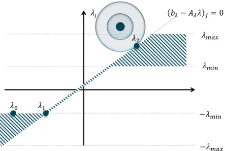
the finitely many faces of the polytopes. From this finite number of affine linear functions one can derive the desired constant l0. For a detailed proof the reader is referred to the monograph [47] and the references therein.

The following lemma is an extended version of proposition 7.2 in [47]. For this we note the KKT system of the QP (3.29):

Qx`c`ATλ´HTµ“0 Axďb Hx“h λTpb´Axq “0 λě0. (3.33)

LetQ, A and H be fixed. We define the following set X

XQP :“ tpc, h, x, λ, µq PR2n`2k`m | pc, h, x, λ, µq is feasible in (3.33)u. (3.34)

3.2 Lemma

Let π be the projection from R2n`2k`m _{to a linear subspace} _Rl_{. Let the} multi-functionF :RlÑR2n`2k`m be defined by

Fpyq “π´1pyq XXQP. (3.35) Then it holds that_F is a polyhedral multifunction.

(48)

3.3. Continuity of the Solution Map and Variational Inequalities 37 Proof Without limitation of generality we assume that πpc, h, x, λ, µq “c. The

graph ofF is then given by

graph_F “ tpc, c, h, x, λ, µq | pc, h, x, λ, µq PXu. (3.36)

Thus it is sufficient to show thatX is a finite union of polytopes. LetsĎ t1, . . . , mu be a subset. We define the set

Gpsq:“XX tpb´Axqi “0 @iPs, λi “0 @iRsu. (3.37) The definition ofGis designed so that within this definition the complementarity constraints in the definition ofXQP (3.33) become redundant. It follows thatGpsq is a polytope. We note that

X “ ď

sĎt1,...,mu

Gpsq _(3.38)

which