Device-free human localization and tracking with UHF passive RFID tags: A data-driven approach
Wenjie Ruan, Quan Z. Sheng, Lina Yao, Xue Li, Nickolas J.G. Falkner, Lei Yang
PII: S1084-8045(17)30422-8
DOI: 10.1016/j.jnca.2017.12.010
Reference: YJNCA 2030
To appear in: Journal of Network and Computer Applications
Received Date: 7 December 2016 Revised Date: 11 July 2017 Accepted Date: 18 December 2017
Please cite this article as: Ruan, W., Sheng, Q.Z., Yao, L., Li, X., Falkner, N.J.G., Yang, L., Device-free human localization and tracking with UHF passive RFID tags: A data-driven approach, Journal of Network and Computer Applications (2018), doi: 10.1016/j.jnca.2017.12.010.
This is a PDF file of an unedited manuscript that has been accepted for publication. As a service to our customers we are providing this early version of the manuscript. The manuscript will undergo copyediting, typesetting, and review of the resulting proof before it is published in its final form. Please note that during the production process errors may be discovered which could affect the content, and all legal disclaimers that apply to the journal pertain.
M
ANUS
CR
IP
T
AC
CE
PTE
D
Device-free Human Localization and Tracking with UHF Passive RFID Tags: A
Data-driven Approach
Wenjie Ruana, Quan Z. Shengb, Lina Yaoc, Xue Lid, Nickolas J.G. Falknera, Lei Yange
aDepartment of Computer Science, University of Oxford, Oxford, OX1 3QD, United Kingdom bDepartment of Computing, Macquarie University, Sydney, NSW 2109, Australia
cSchool of Computer Science and Engineering, The University of New South Wales, Sydney, NSW 2052, Australia dSchool of Information Technology and Electrical Engineering, The University of Queensland, Brisbane, Queensland 4072, Australia
eDepartment of Computing, The Hong Kong Polytechnic University, Kowloon, Hong Kong
Abstract
Localizing and tracking human movement in adevice-free and passivemanner is promising in two aspects:i)it neither requires users to wear any sensors or devices,ii)nor it needs them to consciously cooperate during the localization. Such indoor localization technique underpins many real-world applications such as shopping navigation, intruder detection, surveillance care of seniors
etc. However, current passive localization techniques either need expensive/sophisticated hardware such as ultra-wideband radar or infrared sensors, or have an issue of invasion of privacy such as camera-based techniques, or need regular maintenance such as the replacement of batteries. In this paper, we build a noveldata-drivenlocalization and tracking system upon a set of commercial ultra-high frequency passive radio-frequency identification tags in an indoor environment. Specifically, we formulate human localization problem as finding a location with the maximum posterior probability given the observed received signal strength indicator from passive radio-frequency identification tags. In this regard, we design a series of localization schemes to capture the posterior probability by taking the advance of supervised-learning models including Gaussian Mixture Model, k Nearest Neighbor and Kernel-based Learning. For tracking a moving target, we mathematically model the task as searching a location sequence with the most likelihood, in which we first augment the probabilistic estimation learned in localization to construct the Emission Matrix and propose two human mobility models to approximate the Transmission Matrix in the Hidden Markov Model. The proposed tracking model is able to transfer the pattern learned in localization into tracking but also reduce the location-state candidates at each transmission iteration, which increases both the computation efficiency and tracking accuracy. The extensive experiments in two real-world scenarios reveal that our approach can achieve up to 94% localization accuracy and an average 0.64mtracking error, outperforming other state-of-the-art radio-frequency identification based indoor localization systems.
Keywords: RFID, Hidden Markov Model, Gaussian Mixture Model, Device-free, Indoor Localization, Tracking
1. Introduction
With the explosively increasing aging population, intelli-gent space that can better support the independent living of the elderly has been attracting the increasing attention both from industry and academia. One of the key preconditions for such
5
a smart environment lies on an accurate and timely detection of users’ locations and daily routines [1, 2], especially for an
indoor environmentthat GPS (Global Position System) cannot handle [3]. To tackle this challenge, a wide range of indoor lo-calization and tracking systems have been proposed for the last
10
two decades, including but not limited to LANDMARC [4], WILL [5], Tagoram [6] and BackPos [7]. However most of the approaches are wearable-device based technique that inevitably requires the user to actively carry one or more devices such as various types of sensors, smart-phones, RFID tags/readers or
15
other Radio Frequency (RF) transceivers, thus raising many
in-Email addresses:[email protected](Wenjie Ruan), [email protected](Quan Z. Sheng)
herent impractical issues in reality [8]. For example, the at-tached sensors/tags may be damaged or lost. It is also ob-structive and inconvenient for the user to wear devices all the time1, especially considering that many electronic devices have
20
a moderate size or weight.
For this end, device-free(also calledunobtrusive) passive indoor localization has gained more attention lately and many promising approaches have been proposed [9, 10, 11, 12]. One popular device-free human tracking technique is built upon the
25
recent advance of computer vision, which develops various mod-els to capture human movement from images or videos by us-ing RGB cameras [13, 14], or infrared sensors [15] or depth cameras (e.g., Kinect) [16]. However computer vision based approaches require the tracked user within the line-of-sight2 30
(LOS) of a camera, and usually fail to work in a dimmed en-vironment [13]. Moreover, vision-based technique can also be
1Deloitte Mobile Consumer Survey 2016: www2.deloitte.com/
au/en/pages/technology-media-and-telecommunications/ articles/mobile-consumer-survey-2016.html
M
ANUS
CR
IP
T
AC
CE
PTE
D
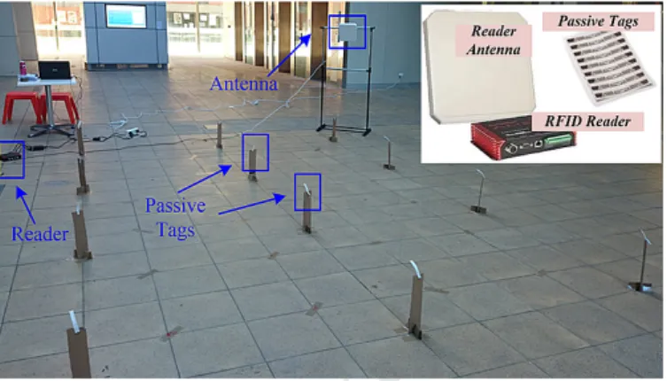
RFID AntennaFigure 1: The general idea of the proposed DfP localization and tracking system
considered to be privacy invasive [1]. Another DfP localiza-tion technique is to intensively exploit the radio-frequency sig-nal,e.g.,localizing the target by analyzing the Received Signal
35
Strength (RSS) variations [17, 18, 2] or Channel State Infor-mation (CSI) [19, 20] in WIFI, or tracking the user through a wall by decoding the radiowaves reflected of human move-ment [21]. Though promising, these systems often require spe-cialized RF signals such as Frequency-Modulated Continuous
40
Wave (FMCW) or build upon costly special-purpose devices such as USRP (universal software radio peripheral), or need to modify the low-level firmware such as abstracting CSI sig-nals. Most importantly, they all require regular maintenance such as battery replacement, thus hindering their practical
de-45
ployment in the real world [1, 8]. In this regard, device-free tracking systems built on COTS (commercial off-the-shelf) pas-sive RFID tags are more promising in terms of deployment convenience (commercialized product without any hardware or firmware modification), maintenance effort (no batteries needed
50
and purely harvesting the in-air backscattered energy) and cost efficiency (≈5 cents each, still dropping quickly) [22, 23, 24, 25]. As a result, in this paper, we design a DfP system that can unobtrusively localize, track a subject to high accuracy based onpurepassive RFID tags.
55
However, applying this high-level idea into a practical in-door localization and tracking system is a non-trivial and chal-lenging task. One key challenge lies on the fact that, in a prac-tical residential environment, RSSI signal is quite complex and unstable because of the multipath effect, power source
fluc-60
tuation and ambient noise disturbance. Unlike the theoretical analysis, the practical RSSI signal however does not strictly de-crease along with tag-reader distance and exhibits significant nonlinearity, and it may be further corrupted when introducing human motion. Another challenging issue is how to model the
65
localization and tracking problem from a data-driven point of view. Currently, most of existing RFID-based systems are built upon the signal propagation model or backscatter communica-tion mechanism, thus there is no off-the-shelf learning-based lo-calization model for us to use. Moreover, to reduce the learning
70
burden, we intend to transfer the pattern learned in localizing a stationary person into tracking a moving subject. Thus how to
effectively bridge the gap between localization and tracking un-der a feasible mathematical framework also deserves a careful resolution.
75
To tackle the aforementioned challenges, we first need to enable the RSSI signal from passive tags to monitor the whole surveillance area in an efficient and unobtrusive manner. Thus we deploy a set of passive RFID tags and a reader (with anten-nas) to form a RSS field that can cover the whole monitored
80
area. Fig. 1 outlines the general hardware deployment in our system. Specially, unlike other RFID-based systems that place the tags on the ground [11, 10], we attach the passive tags and antennas on the wall toi)make the RSSI signal face fewer ob-stacles andii)not obstruct to user’s routine activities, especially
85
in a residential environment. Based upon our RFID infrastruc-ture, some distinguishable patterns can be clearly observed in RSSI signals when a user appears in different locations of a room. In summary, our RFID-based system is intuitively based on two experimental observations:
90
Observation 1. The RSSI vector illustrates differentiable changes when a user appears in an RSS-monitored area comparing to a non-subject scenario.
Observation 2. The RSSI vector reveals distinguishable fluctu-ation patterns when a user presents in different locfluctu-ations within 95
an RSS-monitored zone.
The above two observations substantially illustrate that dis-tributions of a RSSI vector3 are directly relevant with a user’s
indoor positions, and those distributions are differentiable for different locations. Motivated by these two experimental
phe-100
nomena, we thus seek to decode human locations and motions by using data-driven approaches. Specifically, to localize a sta-tionary person, we mathematically formulate it as a classifi-cation problem, in which we first collect the RSSIs and asso-ciated location labels to train a location classifier that is then
105
utilized to predict user’s actual location according to the ob-served RSSI vector (see details in Sec. 4). For tracking a mov-ing user, we first augment the traditionalkNN with probabilis-tic information to quantify the likelihood of locations based on observed RSSIs, which then is utilized to construct the
Emis-110
sion Matrix in HMM. Furthermore, we calculate the Transmis-sion Matrix by introducing two location transition strategies -Constraint-Less Transition(CLT) andConstraint Transition
(CT). The latter transition strategy allows our system to largely narrow down the candidate locations at each state transmission
115
in HMM, which turns out to only not minimize the computation overhead but also increase the tracking accuracy (see details in Sec. 5). At last, we use Viterbi Search to find the most likely path of the subject. We call thiskNN-HMM. In a nutshell, we summarize the main contributions in the paper as below:
120
• We design a device-free indoor localization and tracking sys-tem that utilizes COTS passive RFID tags and bears some
3For example, in Fig. 1, we can formulate the RSSIs of all tags at a certain
M
ANUS
CR
IP
T
AC
CE
PTE
D
Figure 2: Backscatter communication mechanism Figure 3: Path loss illustration Figure 4: RSSI variation with distance
promising characteristics in terms of hardware cost, deploy-ment scalability and maintenance burden. To the best of our knowledge, the designed system, purely built upon passive
125
RFID tags, is one of the device-free works that can not only localize astationaryuser but also track amovingone with a high accuracy in a real-worldresidentialenvironment. • We introduce akNN based HMM method to tracking a motion
person by learning the underlying impacts of a non-moving
130
human body to RSSIs for different locations, which to some extent bridges the gap of localization to tracking from a data-driven point of view.
• We conduct extensive in-suit experiments in a real-world res-idential house where participants unconstrainedly simulate a
135
series of practical daily living routines. The experimental re-sults demonstrate that our system achieves over 94% local-ization accuracy and 0.64mmean tracking error while largely reducing the training overhead to 2 minutes for a17m2
bed-room.
140
We organize the remaining paper as follows. Sec. 2 illus-trates our preliminary analysis and experiential observations. We then mathematically model our target localization and track-ing problems in Sec. 3. In the next, we highlight the proposed solutions in Sec. 4 and Sec. 5. The experimental results are
145
presented in Sec. 6. Then we overview related work in Sec. 7. Finally, some discussions and concluding remarks are offered in Sec. 8.
2. Preliminary
In this section, we will theoretically analyze the RFID
backscat-150
ter radio signal and then verify our system’s capability to reach device-free localization and tracking.
2.1. Backscatter Radio Communication
RFID tags are widely applied in many industries, for ex-ample, an RFID tag attached to an automobile during
produc-155
tion can be utilized to monitored its progress in the assembling, RFID-tagged containers can be tracked during the transporta-tion [26, 27]. Unlike active RFID tags that are powered by batteries, passive RFID systems however communicate through the backscatter radio links due to that passive tags (no
batter-160
ies powered) can only passively collect energy from the in-air
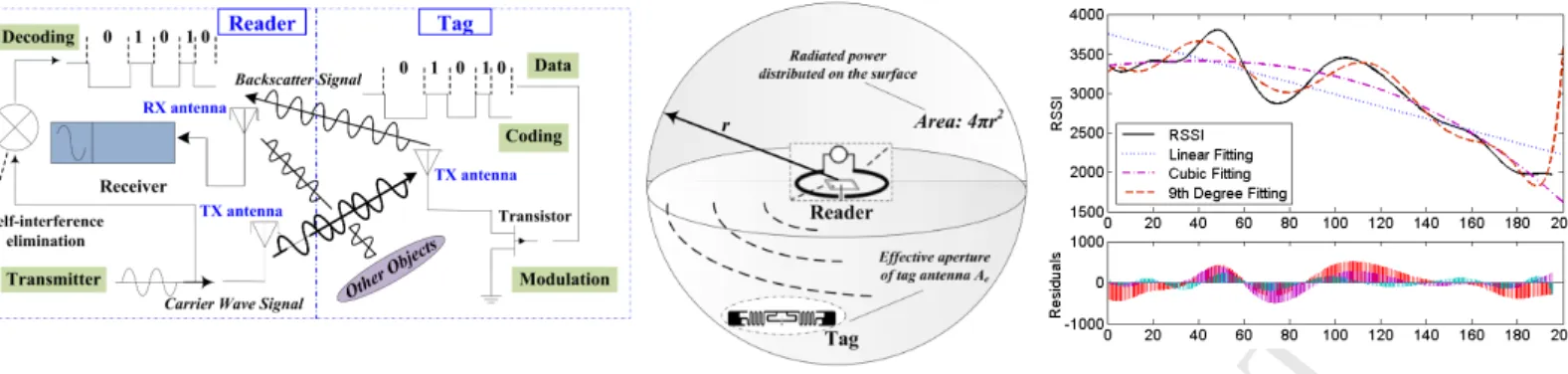
backscattered radio signal. Fig. 2 illustrates a conceptual dia-gram of the radio wave propagation between an RFID reader and a passive tag. In details, the current flow on a reader-antenna induces to a voltage on the tag-reader-antenna (integrated in
165
the circuit), further producing a radiation signal. The radiated wave then makes its way back to the reader-antenna, induc-ing a voltage, thus producinduc-ing a signal that can be detected: a backscattered signal. Specially, the tag transmits “1” bit by changing the impedance on their antennas to reflect the
read-170
ers signal and a “0” bit by remaining in their initial silence state [28], called ON-OFF keying. A typical UHF reader works in the frequency band from 860 MHz∼950 MHz (e.g.,902 ∼
928MHz ISM band in US). Today’s commercialized RFID read-ers have an interrogation distance of about 10meter, which is
175
enough for a residential environment. More importantly, the electromagnetic field produced by RFID readers under no cir-cumstance will harm the human body4.
2.2. Received Signal Strength Indicator (RSSI)
RSSI measures the power of received radio signal between the tag-antenna and reader-antenna [28]. Shown as Fig. 3,Path Lossrepresents the power difference of signals from the receiv-ing antenna and the transmittreceiv-ing antenna. We assume the ra-diated power as being uniformly distributed over a spherical surface at given distancerfrom the reader-antenna. Then, only part of this power is received by a tag-antenna, represented as PRX = PT XAe/4πr2. Since the effective aperture of an an-tenna around a half-wavelength long corresponds to a square round a half-wavelength on a side, the path loss for the isotropic link can be estimated byAe = Gλ2/4πwhereGdenotes the gain of an antenna. Thus we can calculateFriis Equation of the power from the transmission-antennaT X to the receiver-antennaRX[28]. PRX=PT XGT X Ae,RX 4πr2 =PT XGT XGRX( λ 4πr) 2 (1)
Then, we can mathematically model the backscatter signal prorogation as:
PRX,reader=PT X,tagGtagGreader(λ/4πr)2
=PT X,readerTbG2tagG
2
reader(λ/4πr)
4 (2)
4Is RFID Dangerous? www.inria.fr/en/centre/lille/news/
M
ANUS
CR
IP
T
AC
CE
PTE
D
whereGtagdenotes the gain of the tag-antenna andTb
repre-180
sents the loss of backscatter transmission. Thus, under an as-sumption that a wave directly leaves the antenna and strikes the tag (i.e.,interacting with no other objects), Eqn. 2 theoretically demonstrates that the power received by the reader-antenna is inversely proportional to the fourth power of the reader-tag
dis-185
tance. Thereby, for a cleared or open space, RSSIs is capable of being a promising location indicator. However, our system tar-gets to enable a device-free tracking in a cluttered environment. As Fig. 4 shows, the RSSI strength shows a uncertain nonlin-earity with the distance in a residential room, which cannot be
190
expressed by a cubicor even a9th-degree polynomialmodel. So how to model the RSSI-location relation for our application scenario is very challenging. Instead of developing delicate sig-nal propagation models5, this paper intends to seek the answer from a data-driven point of view, i.e.,accurately learning the
195
quantifying relation between the user’s location and the inter-ference of human body to RSSIs from the collected RSSI ob-servations. We will elaborate the details in Sec. 4.
2.3. Intuitions Verification
In this section, we conduct several pilot experiments to
demon-200
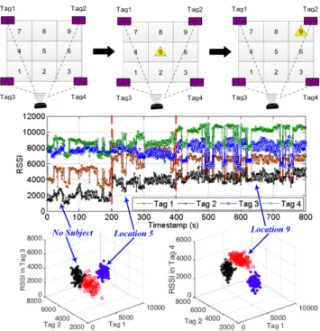
strate the localization potentials of our system. We first build a testbed consisted of one RFID reader and 4 UHF passive tags. The monitored area is divided into 9 virtual grids (0.6m×0.6m each), representing 9 different zonesL1, L2, ..., L9. We want to
verify whether the RSSI patterns reveal distinguishable
differ-205
ences when a user appears in different grids. Fig. 5 snapshots our pilot experimental results. At first, there is no user in the monitored area, then a person stands inL5andL9. We observe
that the measured four RSSI signals obviously vary due to the presence of a subject, so we can clearly discriminate whether
210
there is a subject in the RSS field or not. We also find that the RSSI signal shows different fluctuation patterns when the sub-ject stands inL5andL9. We further cluster the RSSI data
gen-erated from these three scenarios (i.e.,no subject,L5andL9)
into a four-dimension space (illustrated by two 3-D scattering
215
figures). It clearly shows the data clustering in three different subareas (revealing the number of locations the subject ever ap-peared) even without overlapping (can be learned to infer the exact human locations). In summary, the preliminary exper-iments reveal the intuitions and feasibility behind our system
220
for solving the device-free localization. However, in a residen-tial environment, how to accurately decode the accurate loca-tions is still a non-trivial problem considering the complicated multi-path effect and the unstable backscattered RSSI propaga-tion properties. We will elaborate it in Sec. 5.
225
3. Problem Formulation
As aforementioned, we intend to pinpoint the subject’s lo-cations and estimate its continuous trajectory based on the re-ceived RSSIs from a set of RFID tags. Thus we can formally
5This kind of models is also highly related to the furniture and room
lay-out, thereby it is hard to design a physical localization model with satisfying robustness and accuracy.
Figure 5: The RSSI readings cluster in differentiable spaces when a person appears in different locations
define the two targeted problems -localizationandtracking- in
230
this paper as follows.
Problem 1 (Localization). In a monitored area covered by one or more RSS fields, can we accurately pinpoint the current lo-cation of a stationary user given a set of RSSI vectors?
Problem 2 (Tracking). In a monitored area covered by one 235
or more RSS fields, can we continuously estimate the motion trajectory of a moving user with a moderate speed (less than 1m/s) given a sequence of time-tagged RSSI vectors?
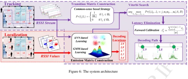
Fig. 6 illustrates the pipeline of our solutions for the two problems. From a data-driven point of view,Problem 1 - Lo-240
calizationcan substantially be reformulated as a location clas-sification problem, in which we aim to accurately quantify the RSSI distributions for different geographical locations within the monitored area. Specifically, assuming thatD anchoring passive tags are deployed in a surveillance area which is
di-245
vided intoGsmall grids, we then can represent the locations as l = {l0, l1, ..., lG} whereli means the subject appears in locationi andl0 indicates the area is empty. In the next, we
collect profiling dataset in the following two steps:i)we record the RSSI readings of all anchoring tags when no human body
250
in the monitored area; andii)then a user appears in location li,(i= 1,2, ..., G)and collect the corresponding RSSI values. Then we build a training datasetH={S0,S1, ...,SG}, where
Si ∈RN×D,Nis the sample number in each grid. This dataset
contains the latent information regarding how a human body
in-255
fluences the RSSIs’ distribution for each location plus an empty environment. We further can quantify the underlying RSSI-Locationrelationship by training a classification model using
M
ANUS
CR
IP
T
AC
CE
PTE
D
Figure 6: The system architecture
localization phase, a user randomly stands on any locations in
260
the surveillance area, and the corresponding RSSI vectors are collected and fed into the location classier. Then it will output location labels that associate with the subject’s actual locations. Assuming that the collected RSSI observation dataset is rep-resented byR={r1,r2, ...,rT}, Problem 1 is mathematically formulated as estimating the optimal posterior probability dis-tributionp(lj|ri)given a RSSI observation sequence.
j∗=argmax
j P r(lj|ri) (3) In Sec. 4, we will give the technical details regarding how to solve the above optimization problem.
265
Similarly, forProblem 2-Tracking, we can model it as es-timating the joint probability distribution upon the RSSI ob-servation sequenceR1:T and the location labelsl1:T where its location state at time-stamptis denoted bylt. We can further simplify the model by assuming that the dynamic motion is a Markov process which only depends on previous location state, represented by modelP r(lj|lj−1). In this end, we need to solve the following mathematical problem:
P r(r1:T, l1:T) =P r(l1)P r(r1|l1) T Y t=2 P r(rt|lt)P r(lt|lt−1) (4) to estimate the expected location statesl1:T with the maximum probability. We also need to train a marginal posteriorP r(si|l1:j) to estimate the expected value ofljgiven observed RSSI read-ings. We will introduce the technical details in Sec. 5.
4. Localizing Stationary Subject
270
This section will introduce three location classifiers,i.e., Mul-tivariate Gaussian Mixture Model, k Nearest Neighbor, and
Kernel-based Localizationfor solving Problem 1 - estimating user’s location given a set of RSSI vectors.
4.1. Gaussian Mixture Model based Localization 275
According to our previous analysis, the key part of local-ization is to model P r(lj|ri), the probability distribution of locations given RSSI observation. This task is difficult since it needs to quantify the distribution of an underlying variable.
However, the reversed distributionP r(rj|li)can be easily learned by observing how RSSIs distribute given the location of a user. Based on theBayes Theorem, we thereby decompose the distri-butionP r(l|r)as follows6:
P r(l|r) =P r(r|l)P r(l)
P r(r) ∝P r(r|l)·P r(l) (5)
where we assumeP r(l)∼1/G, denoting an uniform distribu-tion at locadistribu-tionl. The assumption lies on the fact that a user may appear in any locations with an equal probability. In the next, we need to find an appropriate model that quantifiesP r(r|l)
distribution. Then we can transfer Eqn. 3 as the following opti-mization problem.
l∗=argmax
l∈l P r(r|l)·P r(l) (6)
Figure 7: RSSI distribution pattern and fitted by GMM
In our pilot experiment, we observe that RSSIs display a certain clustering pattern in the high-dimension space. When we take a close look at each cluster, it actually shows a multi-modal distribution that follows a Gaussian Mixture Model, as shown in Fig. 7. This RSSI distribution phenomenon in fact can be explained by the multi-path effect [28, 29]. Normally, several paths for the backscattered signal exist during the prop-agation from a tag to a reader. Among all the paths, the reader prefers to resolve the strongest signal path. When a human
M
ANUS
CR
IP
T
AC
CE
PTE
D
body blocks some propagation paths (i.e.,a subject appears in the RSS field), it will cause the propagation to jump among the multiple paths and lead to the strength migrating from one level to another. As a result, the signal strength exhibits multi-modal characteristics - the distribution is likely composed of multiple Gaussian models. Thus, we can utilize a GMM to cap-ture the probability distribution when a user appears in each grid. Specifically, we propose a Gaussian Mixture Model with mGaussian components as follows:
fl(x) =P r(x|l) = M X m=1 ql,mN(x|µl,m,Σl,m) = M X m=1 ql,m p (2π)D|Σ l,m| exp(−1 2(x−µl,m) TΣ−1 l,m(x−µl,m)) (7) whereΦl = {ql,m, µl,m,Σl,m} represents the model param-eter set for locationl, in whichql,m means the weighted fac-tor for themthmixture component,µ
l,mandΣl,m denote the mean and covariance in themthGaussian component. Further-more, by using the maximum likelihood estimation, the optimal model parametersΦˆlcan be learned through
ˆ Φl=argmax Φl P r(x|l,Φl) =argmax Φl N Y i=1 P r(si|l,Φl) (8) wheres={s1,s2, ...,sN}denotes the training dataset.
To solve the optimization problem in Eqn. 8, we adopt Ex-pectation Maximization (EM), which iteratively optimizes the object function by two steps - E-step (Expectation step) and
M-280
step (Maximization step). Basically, the expectation step cal-culates the posterior probability P r(l|s)by using the training datasets. The Maximization step maximizes the log-likelihood expectation, which in turn enables us to re-calculate the pa-rameters in the following iteration. We use cross validation to
285
find an optimal value of GMM component number that maxi-mize the localization accuracy. With a learned GMM location classier, we can first calculate all the probabilities for candi-date locationsl1:Ggiven an observedr, and then we choose the maximal one as the predicted location of the user.
290
4.2. kNearest Neighbor based Localization
Another way to build a location classier is to learn the Eu-clidean distances of RSSI vectors under a resident appearing on a certain candidate locations. In this regard, we introduce the knearest neighbors (kNN) method that first measures the context-dependent Euclidean distances between a testing RSSI vector with the RSSI vectors of training dataset, and then use a majority vote among its nearest neighbors to assign a location label. Specifically, assuming that we have a training dataset
T = {(s1, y1),(s2, y2), ...,(sN, yN)}withN samples, where
si ∈ RD is the RSSI vector,yi ∈ l = {l1, ..., lG}is the cor-responding location label. Then, given a distance measuring method and a testing RSSI vectorr, we can search itsk near-est neighbors, represented byNk(r). Finally, the testing RSSI
vector is given a most-common location labely∗ among itsk
nearest neighbors by following equation. y∗=argmax
lj
X
si∈Nk(r)
I(yi=lj) (9)
wherej= 1,2, ..., G;i= 1,2, ..., NandIdenotes an indicator
function which is1ifyi=lj, otherwise0.
4.3. Kernel-based Localization
From the point of probabilistic view, if two RSSI vectors have a stronger similarity, then they will be in a near or even same location with a higher probability. Based on this intu-ition, we thus can use a Kernel-based learning (KL) to resolve the posterior probability of candidate locations given an RSSI observation. By applying a kernel function in RSSIs, KL can di-rectly construct possible non-Euclidean topologies that are un-derlaid implicitly in the RSSI vectors and locations. Specifi-cally, in the learning procedure, KL will assign the kernel with a probability mass for every RSSI vector of the training dataset. Then, for an observed RSSI vector, multiple density functions with equal weights will be utilized to estimate the probability. Mathematically, given the training data and corresponding lo-cation labelsS={(s1, li), ...,(sn, ln)}, we can formulate the linear-kernel based localization as the following optimization problem. min w∈Rd,b,ξi wTw+C n X i=1 ξi s.t. li(wTsi+b)≥1−ξi, ξi≥0 fori= 1,2, ..., n (10)
where ξi(i = 1,2, ..., n) are slack variables. C means the error penalty: a small C allows constraints to be easily ig-nored, leading to a large margin, and a large C makes con-straints hard to ignore, leading to a narrow margin. Eqn. 10 es-sentially is a convex optimization problem and there is a unique minimum. Based on the primal-dual relationship, we can opti-mize the model parameters by solving the following dual prob-lem [30]: max µ,α wmin,ξ,b w Tw− n X i=1 αi(li(wTsi+b)−1 +ξi) +C n X i ξi+ n X i=1 µiξi (11)
whereα= (α1, ..., αn)T andµ= (µ1, ..., µn)T are Lagrange
295
multipliers. After learning, in the testing stage, we can feed the RSSI observations into the trained model and output the asso-ciated location labels. In this paper, we adopt LibSVM [30] to realize the KL-based localization. Besides the linear ker-nel shown in Eqn. 10, there are other kernal functions such as
300
polynomial kernel and Gaussian kernel,etc.. The selection of kernel function highly depends on the features of RSSI data and environmental noise causing path loss, and the shadowing and multipath effects in localization. We intensively test the lin-ear kernel, Gaussian kernel, polynomial kernel and radial basis
305
M
ANUS
CR
IP
T
AC
CE
PTE
D
4.4. DiscussionTo summarize, we introduce three different types of local-ization methods. GMM is motivated by the jumping property of backscattered RF signal from tags, which can be explained by
310
the signal propagation mechanism. kNN is based on the sim-ilarity measurement of context Euclidean distance of observed RSSI readings. SVM (support vector machine) is an advanced classification method that are widely adopted by other localiza-tion systems. Actually, there exists other classificalocaliza-tion
meth-315
ods that can be applied into our localization system, such as Naive Bayes, Extreme Learning Machine (ELM),etc. We con-duct some pilot experiments to compare these methods. Specif-ically, we first ask a subject to stand two minutes in each grids to collect the RSSI samples (the testbed is shown in Fig 5),
320
then we randomly divide the dataset into training and testing datasets in different ratios (from 10% to 90%) to test the meth-ods. As Fig. 8 shows, among all the classification methods, k Nearest Neighbors achieve the best result. Even with only 10% training data (12 seconds in each grid), it reaches 87.2%
325
accuracy (greatly simplify the pre-calibration and relieve our training burden). It reveals that, with only a few labeled RSSI data, the context-dependent distance measurement can better interpret the fluctuation of RSSI signal caused by human body inference, which strongly motivates our kNN-HMM to tackle
330
the tracking problem.
Figure 8: Localization results of different methods
5. Tracking a Moving Subject
Comparing to localizing a relatively static user, human track-ing is more challengtrack-ing, especially considertrack-ing the sudden and unpredictable RSSI changes caused by a moving human body,
335
which makes the RSSI-Location mapping more difficult. How-ever, on the other hand, within a sampling time, the next mov-ing location will be near to the current location due to the hu-man speed limitation (≤1m/s), which naturally narrows down the possible candidate locations. In other words, for tracking
340
problem, we have one more evidence, namelycurrent location state, that can help us to infer the possible locations besides the RSSI observations. Specifically, we propose two HMM-based models, kNN-HMMandGMM-HMM, to decode the continu-ously time-stamped RSSIs into the subject’s moving path by
345
considering both patterns learned from localization model and
the location transition constraints. Hidden Markov Model is widely applied in spatio-temporal pattern recognition such as handwriting recognition, proteins structure prediction and hu-man activity recognitionetc.. It can be considered as a
gener-350
alization of a mixture model where the latent variables, which control the mixture component to be selected for each observa-tion, are related through a Markov process rather than indepen-dent of each other. In this regard, HMM is perfectly fit the as-sumption of our tracking problem that the next moving location
355
depends and only depends on present location, neither being to-tally independent nor related to the past location states. Another challenge in tracking is the latency, namely the subject already moves to next location whiles the system is calculating the cur-rent location. To reduce this disturbing phenomenon, given the
360
resulting continuous location points from HMM-based models, we further design a forward calibration mechanism that sub-stantially takes account of a few past location estimations when resolving current location. In the next, we will elaborate the details of kNN-HMM based and GMM-HMM based tracking
365
methods as well as the forwarded calibration mechanism. Assuming thatLrepresents all candidate user’s moving tra-jectories and R denotes the observed RSSI vector sequence, then our primary goal is to optimize a trajectoryL∗with a max-imum likelihood based on the following equation.
L∗=argmax
L P r(L|R) (12)
According to Bayesian Theorem, we transform optimizing the conditional distribution into finding an optimal joint proba-bility distribution.
P r(L|R) = P r(L,R)
P r(R) ∝P r(L,R) (13)
Assuming that Ris consisted ofT time-tagged RSSI ob-servationsr1:T andLcontainsT corresponding location states l1:T, we can further decode Eqn. 13 as follows:
P r(r1:T, l1:T) =P r(l1)P r(r1|l1) T Y t=2 P r(rt|lt) | {z } B P r(lt|lt−1) | {z } A (14) Now we successfully model our tracking problem as a Hid-den Markov Model. To solve the model, we first need to esti-mateTransition MatrixAandEmission MatrixBand then use
Viterbi Searchto find the optimal location trajectory.
370
• Transition Matrixcaptures state-transition probability of a user moving from a location-state lt−1 at time-stamp
t −1 to a location-statelt at time-stamp t. It can be represented viaP r(lt|lt−1).
• Emission Matrixmodels the probability of observing RSSI
375
vectorrtgiven a location stateltat time t, denoted by P r(rt|lt).
• Viterbi Searchingfinds a location sequence{l1, l2, ...lT} that has a maximum likelihood given Transition Matrix Aand Emission MatrixB.
M
ANUS
CR
IP
T
AC
CE
PTE
D
5.1. Transition MatrixFirst of all, we show how we build a transition matrix based on the location state constraint. Generally, the human motion can be seen as a state transition process that next moving loca-tion is solely dependent of current state but irrelevant to other
385
states, which can be defined by a probability matrix Aij = P r(at = li|at−1 = lj). To construct such a matrix, we de-fine following two human motion patterns based on an intuition that a person is only able to move a limited distance during one sampling interval (i.e.,0.5secondin our system) given the
390
moving speed (≤1m/s) in an indoor environment.
• Constraint-Less Transition (CLT): The tracked user can move to any locations of the monitored area under a same likeli-hood, namelylt∈l0:Gwith an equal probability.
• Constraint Transition (CT): The tracked user can only move
395
to one-sampling-time reachable locations of the monitored area under a same likelihood and cannot reach other loca-tions.
The second motion pattern greatly facilitates the tracking efficiency due to the fact that it can largely exclude some un-likely location states in each calculating iteration. For example, in Fig. 12, it is impossible for a resident to move fromL11to
L64within 0.5 second, so we can eliminateL64from the next moving locations whilst user’s current location isL11. In this paper, we categorize the one-sampling-time reachable locations as those grids that are adjacent or equal to user’s current loca-tion. Mathematically, we formulate these two transition pat-terns by one equation. We assume that the monitored area is di-vided intoGlocations andli(i= 1,2, ..., G)means the tracked user is in gridi. According to the proposed two motion patterns, we further define a location-state setΩi including all feasible states that a user can move to given current state li, and use
|Ωi|to denote the number of states. We then can construct a transition probability matrix as follows:
P r(lj|li) = 1 |Ωi| iflj ∈Ωi 0 iflj ∈/ Ωi (15) 5.2. Emission Matrix
As Eqn. 14 shows,Bij =P r(ri|lj)represents the emission
400
matrix that essentially shares the same purpose as the localiza-tion problem - modeling the RSSI distribulocaliza-tions for different lo-cation states. As a result, we can construct the emission matrix by taking advantage of aforementioned localization models.
5.2.1. GMM-based Emission Matrix 405
One straight-forward way is to construct the emission prob-ability matrix based on the GMM model, which is capable of estimating emission probabilities given the RSSI observations. Similar to localization problem, we assume that the probability distribution of RSSI observations follows a multivariate
Gaus-410
sian Mixture Model for each location state, and we thus are able to calculate the Emission Matrix using Eqn. 7.
5.2.2. kNN-based Emission Matrix
Another way to construct the emission matrix is taking the merit ofknearest neighbor model which reveals a superiority in
415
mapping the RSSI observations with the latent locations. To do so, we construct a kNN-based emission matrix by transforming a traditional kNN classier into a probabilistic style that can give an emission probability conditioning on the observed RSSIs.
Specifically, the probabilistickNN estimates theEmission Matrixas follows. We first search the top-knearest neighbors N(rj)in the profiling dataset for observed RSSIrj. Then we also mark these searched samples by its belonging locations, represented byNi(r
j) ={sk|sk∈ N(rj)∩sk ∈li}. Then the probabilistickNN-based emission matrix is built as follows:
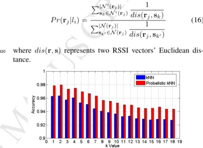
P r(rj|li) = P|Ni(rj)| sk∈Ni(rj) 1 dis(rj,sk) P|N(rj)| sk0∈N(rj) 1 dis(rj,sk0) (16)
where dis(r,s) represents two RSSI vectors’ Euclidean
dis-420
tance.
Figure 9: Localization accuracy comparision withkchanges
We conduct a pilot experiment to compare probabilistickNN and transitionalkNN as well. We first collect 2 minutes training data in each grid, then use 40% as the training data and 60% as the testing data to test the methods. As Fig. 9 shows, the
425
proposed probabilistickNN method slightly outperforms tradi-tionalkNN in allkvalues. More importantly, the probabilistic kNN is capable to estimate the posterior possibilities by mea-suring the context distances. Overall its advantages lie in: i)it specifically gives the posterior distribution of each class rather
430
than assigning a class-membership to the test sample; andii)it assigns each neighbor a weight that is inverse-proportional to its distance with the test sample, which not only considers the number of its most-common neighbors but also measures their relative distances.
435
5.3. Viterbi Searching
Given a sequence of observations, Viterbi searching, one of dynamic programming algorithms, can find an optimal se-quence of hidden states with a maximum likelihood, especially being efficient in solving HMM. Specifically, assuming that the length of time-stamped RSSI observations istand the ending location state islj, Viterbi searching finds the most likely se-quence of latent location states as following induction process.
M
ANUS
CR
IP
T
AC
CE
PTE
D
Figure 10: HMM based methods
Vj(t) = arg max l1,l2,...,lt−1
P r(l1l2...lt=j,r1r2...,rt|A, B) (17) where matrix A and B refer to Eqn. 14. By induction, we further obtain:
Vj(1) =Bj(r1) Vj(t+ 1) = arg max
i Vi(t)AijBj(rt+1)
(18)
where Bj(r1) = P r(r1|lj)andAij = P r(lj|li). After the induction calculation, we finally can search an optimal mov-ing trajectory for both GMM and kNN based HMM methods. Fig. 10 sketches these two HMM-based methods for dealing
440
withTracking.
5.4. Latency Reduction
As aforementioned, another challenge we need to deal with in tracking is the latency, which mainly results from the delay of RSSI collection and signals sending by passive tags [28]. As a result, we introduce aforward calibrationmechanism to re-calibrate the walking trajectory outputted by the Viterbi search-ing to reduce the latency. Specifically, we adopt a slidsearch-ing win-dow to average the latest several locations as follows:
ˆ c0t= Pt+|w|−1 i=t ˆci |w| (19) whereˆc0
trepresents the calibrated coordinates of locationltis the at timet,|w|denotes the length of the sliding window, and
ˆ
ciis raw coordinates of estimated grid’s center at timeiusing
445
Eqn. 17.
6. Evaluation
We evaluate our approach throughi)micro experiments in a
3.2m×4.8mtesting area (stacked by 6 RSS fields); andii)field experiments in a fully furnished house including two bedrooms
450
and a kitchen (around220m2gross floor area). 6.1. Hardware and Software Platform
Ultra-low cost of UHF tags (5∼10 cents each) become the preferred choice of many industry applications. Following the common practices, we adopt passive UHF tags in this paper.
455
Figure 11: Hardware deployment
As Fig. 11 shows, our system is built upon commercial off-the-shelf RFID products without any hardware or firmware modifi-cation. Specifically, we use an Alien ALR-9900+ RFID reader, several reader-antennas (Model: ; Size:20cm×20cm×3cm) and dozens of UHF passive tags (Model: squiggle Higgs-4;
460
Size: 1cm×10cm). The operation frequency of the reader is 840 to 960MHz and the sampling rate is 2Hz. Each collected RSSI readings includes a TAG-ID, RSSI and TIME. Our system runs in a laptop computer (CPU: I7-3537U 2.5GHz; RAM: 8G; OS: Win7). The software for RSSI data retrieval is written by
465
C#and uses the API provided by Alien company. The back-end data analysis and modeling are based on Matlab 2016a.
6.2. Evaluation Metrics
Similar to other localization and tracking systems, we adopt the following two evaluation metrics,AccuracyandError Dis-tance, to measure the localization accuracy and tracking error respectively.
Acc.=
PN
i I(ˆli, li)
N (20)
whereˆliandlirespectively denote the estimated and actual lo-cation of a user, the indicator function I(a, b) equals to 1 if
a = b, otherwise0, andN denotes the tested RSSI numbers. The tracking error distance is defined by
Derror=
P|T|
i dis(ˆci, ci)
|T| (21)
The error distance depicted above actually measures the av-eraging accumulated error distance for each moving trajectory.
470
Specifically,ciandˆcimean the actual and predicted coordinates of a subject at timei, anddis(ˆci, ci)denotes the Euclidean dis-tance between them. |T|is the number of all observed RSSIs of a moving trajectory.
6.3. Micro Experiments 475
We first conduct several micro experiments to test our meth-ods. Before evaluating our approaches, we need to decide how to choose the optimal size for each virtual grid. This paper aims to support the independently living for the elderly in a res-idential environment. So we choose the size of grids based on
M
ANUS
CR
IP
T
AC
CE
PTE
D
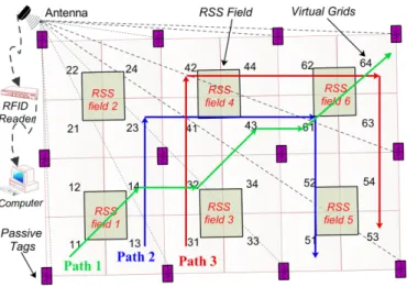
Figure 12: Multiple RSS fields and testing paths
the requirement of a specific application. Based on our exper-iments, a grid with too small size (e.g.,0.1m×0.1m) would increase the calculation overhead and need more profiling data (for training the model), because a small grid size brings more indistinguishable patterns. On the other side, a grid with too
485
large size (e.g.,2m×2m) may lead to a coarse-grained local-ization, for example, a regular bedroom with 10 square meters can only be divided into 2 grids, leading to a room-level lo-calization. As a result, we need to wisely choose the grid size based on the specific requirement of a real-world application.
490
In this paper, a very high location resolution is not our primary goal. For example, caregivers normally more concern about the elderly resident locating on which area or room of a house or apartment instead of an extremely fine-grained location point. Based on this intuition, we setup our experiments as Fig. 12, in
495
which each virtual grid is0.8m×0.8m, locating people in a
0.64m2resolution.
6.3.1. Experimental Settings
As Fig. 11 shows, one reader-antenna is placed at1.55m height and faces to passive tags from 25◦ ∼75◦ angle7. The
500
tags are attached on paperboard-holders placed30cmabove the ground. Considering that our model aims to learn the RSSI-Location mapping, those passive tags can be flexibly put as any geometric shape. For simplicity, we deploy the passive tags as a square array with around1.6mdistance. Another issue is that,
505
the reader may lose some RSSI readings due to the human body occlusion during localization or tracking. As a result, to make the received RSSI vector with same number of readings, we fill in those missing values as 0 in each sampling time.
6.3.2. Localization 510
To test the localization capability, we define three scenarios to simulate the possible real-world daily routines.
Scenario 1 (Stationary). A person stands or sits statically in a certain location of monitored area, mimicking that a resident may talk with someone or watch TV.
515
7The antenna angles or height can be set up arbitrarily as long as it is able
to capture all the readings of all tags in an empty environment.
Table 1: Localization accuracies of different methods by using different ratios of training data Scena. Ratio (%) 10 20 30 40 50 60 70 80 1 kNN 0.946 0.954 0.958 0.958 0.960 0.961 0.962 0.963 GMM 0.927 0.935 0.938 0.940 0.939 0.943 0.940 0.941 SVM 0.707 0.756 0.823 0.851 0.897 0.912 0.919 0.928 ELM 0.664 0.764 0.719 0.771 0.881 0.898 0.904 0.904 NaiveBayes 0.883 0.887 0.913 0.930 0.938 0.944 0.943 0.946 2 kNN 0.810 0.823 0.833 0.844 0.869 0.902 0.913 0.931 GMM 0.751 0.777 0.783 0.793 0.838 0.884 0.894 0.902 SVM 0.656 0.717 0.775 0.797 0.819 0.832 0.846 0.857 ELM 0.680 0.538 0.614 0.701 0.677 0.774 0.819 0.835 NaiveBayes 0.741 0.777 0.793 0.844 0.872 0.890 0.903 0.914 3 kNN 0.880 0.904 0.918 0.927 0.931 0.931 0.936 0.943 GMM 0.851 0.877 0.883 0.893 0.898 0.904 0.904 0.912 SVM 0.715 0.746 0.774 0.826 0.840 0.854 0.876 0.881 ELM 0.688 0.583 0.617 0.693 0.705 0.812 0.840 0.846 NaiveBayes 0.768 0.789 0.855 0.889 0.918 0.921 0.928 0.929
Scenario 2 (Dynamic). A person moves around and does sev-eral activities within a certain small zone, mimicking a resident may cook in the kitchen or do morning exercise.
Scenario 3 (Mixed). A subject performs both activities defined in Scenario 1 and 2 within a certain location.
520
Accordingly, we test our system based on the above three scenarios:i)a participant appears in each location for120s;ii)a participant walks around and performs some activities in each grid for120s; andiii) a participant does the above activities for 240sper grid. Overall we collect 276,480 RSSI readings
525
in the localization experiments. We randomly split it into test-ing and traintest-ing datasets based on different ratios (in each ratio, we run the methods twenty times to calculate the average local-ization accuracy). Table 1 compares our experimental results of five localization methods with different training ratios. We
530
carefully tune the parameters for each method - we setk = 2
forkNN and GMM component number as 4, and choose termi-nation criterion and C in SVM with a linear kernal as 0.01 and 1 respectively [30]. For a stationary scenario, all five meth-ods can localize the subject with a decent accuracy. Among
535
all, kNN classifier achieves a 94.6% localization accuracy in particular with12s/gridtraining data, which significantly out-performs other methods especially the SVM and ELM. For a challenging dynamic localization scenario,kNN still achieves a better performance with 93.1% accuracy using 80% training
540
data. It is also noted that, under adynamicscenario, the local-ization accuracy is more relevant to the training data size. A larger training dataset is able to provide more informative RSSI patterns for this case. In Scenario 3, our system is able to reach a high accuracy of 94.3%. In summary, under a circumstance
545
of limited training data (e.g.,10% training data), kNN based localization reveals a better and robust performance. It is worth to mention that, to achieve a similar accuracy, the shortest col-lection time of training data is ofminutes-levelin past localiza-tion systems [31]. On the contrary, our system only requires a
550
seconds-levelcollection time to get a comparable localization performance. We also observe that, with more training data (e.g.,80% training data in Table 1), other methods are also able to get good accuracy but more sensitive to the training data size.
M
ANUS
CR
IP
T
AC
CE
PTE
D
Figure 13: Tracking errors on three paths (CT:
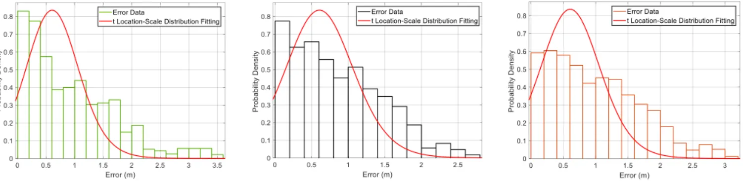
Con-straint Transition; CLT: ConCon-straint-Less Transition) Figure 14: Average tracking errors Figure 15: The error data andtLocation-Scale Dis-tribution fitting for kNN-HMM + CT
6.3.3. Tracking 555
In the tracking experiments, we evaluate our HMM based models on three moving trajectories8 under the proposed two
transition strategies, illustrated in Fig. 12. Two persons with various weights and heights participate our experiments and ev-ery path is tested for 20 times9. As Fig. 13 illustrates,
kNN-560
HMM with Constraint Transition (i.e., kNN-HMM + CT) is able to track a subject with 0.64m mean error, achieving the best result among all the methods. This may lie in the fact that kNN-HMM + CT feasibly narrows down the candidate loca-tions (excluding the invalid location candidates), thus can better
565
quantify the mapping relation from RSSI sequence to moving trajectories. We also compare our system with other popular RFID-based localization works, as shown in Fig. 14.
LANDMARC[4] is the very first RFID-based localization system that tracks a tagged subject by measuring its weighted
570
average locations of its nearest four tags. It needs the target at-tached with tags and know the reference tags’ locations. In our experimental testbed, it achieves average tracking error 1.64m (i.e.,LANDMARC-1: 3×4 reference tags with 1.6minterval), and 1.11m(i.e.,LANDMARC-2: 5×7 reference tags with 0.8m
575
interval).
TagArray[11] is one of the first RFID-based systems that can localize a subject in a device-free manner. Generally, TagAr-ray detects a person by comparing the variation of RSSI read-ings with a pre-learned threshold. However it is built upon
ac-580
tive RFID tags and requires a high tag tensity as a tag array. It reaches 1.7m(i.e.,TagArracy-1: 3×4 reference tags with 1.6m interval) and 1.15m(i.e.,TagArray-2: 5×7 reference tags with 0.8minterval) mean tracking error in our testbed.
TASA[10] is another device-free RFID-based localization
585
system, which adopts both passive and active tags. Thus it is less costly than TagArray. But still, it requires to calibrate all tags’ coordinates. It gives 1.53m(i.e.,TASA-1: 3×4 reference tags with 1.6minterval) and 1.05m(i.e.,TASA-2: 5×7 refer-ence tags with 0.8minterval) mean tracking error.
590
8During the experiments, we do not specifically require the testing
partici-pants to walk through the centre of each grid, we just set predefined trajectories and each trajectory is composed by several grids, which is later used as ground truth labels for model evaluation.
9We mainly focus on tracking a resident with a moderate moving speed
(≈0.6m/s) due to that fast moving in an indoor environment is not practical.
SCPL[9] is one of the advanced wireless-based device-free localization systems. It utilizes a Gaussian model based Con-ditional Random Field (GM-CRF) method to track a moving person. It is very similar to our GMM-HMM method (utilizing Gaussian Mixture Model). We implement the GM-CRF method
595
in our RFID dataset and get a mean 0.98mtracking error.
Twins[22] is a very recent RFID-based system purely built upon passive tags, which utilizes a interference phenomenon (called state jumping) of two passive RFID tags to do the mo-tion detecmo-tion. It gives a mean 0.75mtracking distance error in
600
an open warehouse. Twins also needs to carefully calibrate the positions of the reference tags.
BackPros [7] is one of the recent RFID-based positioning systems, which is able to track a passive tag with a decimeter-level accuracy. However, BackPro aims to track an object
in-605
stead of tracking a human body by exploring the phase differ-ences of backscatter signals to infer the tag’s location. It needs to carefully calibrate the positions of four antennas beforehand and the tracked object need to be attached with a passive tag.
Different to the baseline methods, our system does not need
610
to calibrate the tags’ locations10 and achieves 0.64m average
tracking error in our testbed. It offers about 2.56×, 2.66×, 2.39×and 1.53×improvement compared with LANDMARC [4], TagArray [11], TASA [10], SCPL [9] (see Fig. 14) using the same number of tags. Fig. 20 shows the CDF (cumulative
dis-615
tribution function) curves of tracking error for different meth-ods. ThekNN based HMM with CT achieve a better result, nearly 76% tracking errors are below 1m.
6.3.4. Evaluation bytLocation-Scale Distribution Fitting
In this section, we compare our system with baseline
meth-620
ods in terms oftLocation-Scale Distribution Fitting. This idea is first introduced by [32]. The author argue that, for a small testing dataset, it is necessary to adopt a performance evaluation criteria that can approximate the actual performance of system in practice. Similar to thet-distribution fitting based method
625
proposed in [32], in this paper we first utilizetLocation-Scale Distribution (an extension oft-Distribution) to fit those error
10Although we put tags in a square array in Fig. 12, we actually do not use
any coordinates of the tags. Because we target to learn the mapping model, the tags can be placed in other geometric locations.
M
ANUS
CR
IP
T
AC
CE
PTE
D
Figure 16: The error data andtLocation-Scale Distri-bution fitting for kNN-HMM + CLT
Figure 17: The error data andtLocation-Scale Distri-bution fitting for GMM-HMM + CT
Figure 18: The error data andtLocation-Scale Distri-bution fitting for GMM-HMM + CLT
Figure 19: The stand derivation and mean value oftLocation-Scale Distribution fitting for
baseline methods Figure 20: Tracking error CDF
datasets produced by different localization methods. Then we compare the standard derivation and mean values of those dis-tributions fitted.
630
The probability density function (PDF) of the t location-scale distribution??is f(rerr) = Γ(ν+1 2 ) µ√νπΓ(ν2) 1 + (rerr−µ) 2 σ2ν −ν+12 (22) wherererrindicates the error data,Γ(∗)represents the gamma function,µis the location parameter andσmeans the scale pa-rameter,ν is the shape parameter. Actually, we can transfert
location-scale distribution into a Student’st-distribution when parametersµ= 0andσ= 1.
635
Fig. 15∼18 illustrate the probability densities along with error distances for kNN-HMM + CL, kNN-HMM + CLT and GMM-HMM + CL as well as kNN-HMM + CLT, and the cor-responding tlocation-scale distributions fitted. Fig. 19 shows the standard derivation and mean values of the distributions for
640
all the compared methods. As we can see, the proposed method, kNN-based HMM with Constraint Transition, achieves a lower mean and standard deviation values.
6.4. Field Experiments
This section delivers the experimental results in a residential
645
house that contains 2 bedrooms (i.e.,a home office and a master room) and a kitchen, as shown in Fig. 24. The reader-antennas are deployed around 1.7metersvertical distance to the ground
and the facing angle to the passive tags is around60◦, which is capable of capturing all RSSI readings under a non-resident
650
environment. Overall we virtually divide the monitored area into 25 grids, and use 34 passive RFID tags and one reader with three antennas. We attach those passive tags on the room-walls with about0.8minterval.
6.4.1. Localization 655
Similarly, we design three localization scenarios in our field experiments - Stationary, Dynamic andMixed. Accordingly, three types of data are collected to train and test the location classifiers11.
Figure 21∼23 show the results of localizing a subject using
660
five different location classifiers varying training ratios (from 5% to 90%)12. In thestationary scenario, the localization
ac-curacy ofkNN is as high as 93.8% with 90% training ratio. More importantly, only with 6 seconds training data (5% train-ing ratio) for each grid, it can achieve an accuracy over 85% in
665
a residential house, revealing its advantage than other location classifiers. For Scenario 2, the performances of all methods are
11i)a person appears in each grid for 120s,ii)a person contentiously moves
round in a grid for 120s, andiii)a participant does the above stationary and dynamic activities respectively for 120s. For L1, L10, L11, we only collect the data people lying down for all scenarios. Overall, we collect 848,640 RSSI readings, forming 24,960 RSSI vectors.
12We randomly choose the training dataset and testing dataset, and conduct
M
ANUS
CR
IP
T
AC
CE
PTE
D
Figure 21: Localization accuracy in Senario 1 Figure 22: Localization accuracy in Senario 2 Figure 23: Localization accuracy in Senario 3
Figure 24: House layout and tracking paths
Figure 25: Tracking errors on three paths
degenerated due to the unstable human inference, and the re-sults among different methods are more close to each other. We also observe that more training data can significantly enhance
670
the localization accuracy, which means, for the challenging dy-namic scenario, collecting more training data can more accu-rately capture the human inference to RSSI signals. For Sce-nario 3, the best perfermance is achieved bykNN using 90% training data, and the overall performance is betweenstationery 675
scenario anddynamic scenario. In summary, kNN shows its superiority in RFID-based device-free localization, considering its simplicity, light computation overhead and relaxing require-ment of training data.
6.4.2. Tracking 680
We also test our tracking methods on three daily routines, shown as Fig. 24.
Path 1:L10→L9→L17→L25→L24→L23→L21→
L20represents that, a resident gets up from the master room and does some cooking in the kitchen.
685
Path 2: L4 → L5 → L6 → L7 → L8 → L9 → L16 →
L15→L12mimics that a resident gets up from the sofaL4of the master room, and then goes to work at the deskL12of the home office (i.e.,the room in the upper-left of Fig. 24).
Path 3: L11 → L12 → L15 → L16 → L17 → L18 →
690
L19→L20 →L21 →L22indicates that, a resident gets up from the bedroom and goes to the kitchen using the kettle.
Overall three subjects join the experiments and each path test is repeated 20 times. As Fig. 25 depicts, our proposed kNN-HMM with Constraint Transition illustrates a better result (with
695
1.07mmean tracking error) comparing to other HMM based
models. It is noted that, in Path 3 - a more complex path of daily routine, our method obtains a larger tracking error (nearly 1.2m). The reason may be due to the fact that Path 3 involves walking through a narrow hall with many electronic appliances
700
in the kitchen, which block or absorb the energy of backscat-tered signal from an antenna. Thereby the tracking accuracy decays for this application scenario. In general, our proposed method outperforms other methods by intensively learning the mapping relation between RSSI readings and human mobilities
705
under a transition constraint. It is noted that SCPL achieves 1.66mmean error, 1.55 times larger than our method. In the field experiment, we only compare our system with the pro-posed method in SCPL since the LANDMARC, TagArray and TASA place the RFID tags as arrays on the ground. Such
de-710
ployments are impractical and obtrusive for a residential envi-ronment. Firstly, the reader even cannot catch the readings from passive tags that are deployed in a carpet ground since signals are blocked by furnitures around and absorbed by the carpet. Secondly, tag-arrays that densely deployed on ground in a
res-715
idential environment strongly obstructs the mobility of the res-ident, causing uncomfortable and inconvenient. In our system, the passive tags are attached on the wall which is more practi-cal and considered as less intrusion. As a result, the lopracti-calization systems proposed in LANDMARC, TagArray and TASA are no
720
longer capable for the residential application scenario.
6.5. Parameters Selection
In this section, we will discuss the factors that have impact on the tracking accuracy.
M
ANUS
CR
IP
T
AC
CE
PTE
D
6.5.1. Tag Density 725Tag density is an important influential factor to the tracking performance. As Fig. 26 shows, we investigate the impact of tag density by deploying different numbers of tags in the testing rooms. The experiments reveal that a sparse tag density (e.g.,2 tags/room) will reduce the tracking performance. On the other
730
side, continuously using more passive tags does not improve the tracking accuracy significantly. For example, in our exper-iments, the tracking error does not decrease obviously when increasing the tag number from 34 to 89. Such a phenomenon lies in a fact that it is difficult for an antenna to probe a large
735
number of passive tags and thus resulting in severe reading loss. It is noted that, comparing to TagArray and TASA that require a high density of tags, our system is able to achieve a comparable tracking accuracy using less passive tags.
6.5.2. kValue and GMM Component Number 740
There are two key parameters in our HMM-based models, one iskvalue in Emission Matrix ofkNN-HMM, another one is thecomponent number(CN) of GMM in GMM-HMM. We in-vestigate these two parameters in our micro experiment testbed. Fig. 28 illustrates that, the tracking error reaches the lowest
745
when k = 7, which thus is chosen as the optimal value in our tracking system. However, GMM-HMM achieves a bet-ter tracking accuracy at CN = 4, 8, 9 and 15. Considering that a larger CN may potentially cause a model over-fitting and re-quires more computation overhead, we choose CN = 4 in this
750
paper.
6.5.3. Window Length
For a localization system, dealing with the latency is also a concerning issue [33, 1]. In this paper, we introduce a sim-ple yet efficient forward calibration to reduce the latency,
lay-755
ing on the fact that previous human motion has an impact on current location prediction. One of key parts is to decide the length ofprevious motion,i.e.,the smoothing window length. Fig. 29 shows the relevance between the window size of for-ward calibration and the tracking error in different paths using
760
two HMM based methods. We observe that, when the window length ranges from 8 to 11, our system achieves a less tracking error. Thus, we select 8 as the optimal length in our system considering both the computational burden and accuracy.
6.5.4. Stationary DatavsDynamic Data 765
As mentioned before, we put two kinds of training data into the HMM based methods - stationary data (Scenario 1) and dy-namic data (Scenario 2). In order to analyze which type of train-ing data plays a key role in tracktrain-ing, we first add 120 seconds
dynamic training data (before black dot line, the First-stage 770
Training), then we add another 120sstationary data for train-ing (after black dot line,the Second-stage Training), shown as Fig. 30. Overall, we observe that the tracking error decreases as adding more training data. In details, the error diminishes rapidly in the first stage, but just slightly reduces in the
sec-775
ond stage. Actually, the last 72 seconds stationary data does not make much contribution to improving the performance. It
reveals that more dynamic data substantially provide richer an-choring RSSI information regarding the human motion, and a few stationary training data (e.g., collecting 24 seconds
train-780
ing data) nearly provide all the essential statical information for tracking. In other words, we can add more dynamic training data to improve the system’s tracking performance.
6.6. Computation Complexity 785
The proposed traking method is based on the framework of Hidden Markov Model and use a Viterbi Searching to de-code the user’s trajectories. The complexity of our algorithm is O(T×S2), whereT is the number of RSSI vectors observed
andSis the number of location states, which is 26 in the field
790
experiments. Thus our algorithm has a linear complexity with respect to the length of observations, which is efficient enough given the advances of current COTS computers. Actually, some baseline methods such as LANDMARC is simpler, which is only based on k Nearest Neighbors without any dynamic
pro-795
gramming algorithms for sequence matching.
7. Related Work
This section will review the related works regarding indoor localization and tracking. Generally, they can be categorized aswearable-device based localizationanddevice-free localiza-800
tion. We will focus more on the device-free techniques that is more related to our system.
7.1. Wearable Devices based Localization
Wearable device based systems normally requires the user to carry or wear a device such as RF transceivers, smart-phones,
805
RFID reader or tags. The very first indoor localization work is Criket [39] which is able to track a subject wearing an ultrasonic transmitter by measuring the ToA (time-of-arrival) of a short ul-trasound pulse. Another very famous pioneering work, LAND-MARC [4], first deploys dozens of active RFID tags in the
in-810
door environment, and then match the RSSI from a tag carried by a subject with the profiled RSSI fingerprints to localize a tar-get. Lately, Yang et al. [6] design a high-performance tracking system based on passive RFID hardware, which can real-time track a tagged object with a centimeter-level error. With the
815
popularity of smart phones, Zhou et al. [40] present an activity sequence-based pedestrian indoor localization approach using smartphones. They first detect the activity sequence using activ-ity detection algorithms and use HMM to match the activities in the activity sequence to the corresponding nodes of the indoor
820
road network. MaLoc [41] utilizes magnetic sensor and inertial sensor of smart-phones by a reliability-augmented particle fil-ter to localize a subject, which does not impose any restriction on smart-phones orientation. Currently, wearable device based localization is still a very active research area due to its high
825
accuracy and robustness. However, the requirement of wearing a sensor or device may be not practical for some circumstances.
M
ANUS
CR
IP
T
AC
CE
PTE
D
Table 2: Comparison of typical device-free localization systems
Comparison Systems Measured Physical Quantity Non-LoS Localization? Hardware Cost of Single Node/Device Localization Accuracy System Scalability Maintenance (e.g.,replace batteryetc.) Training Overhead Tested in a Residential Home? Device -free? TagArray[11] RSS Threshold NO Active Tags Medium Medium Medium Medium Low NO YES
TASA[10] RSS Threshold NO Passive and
Active Tags Medium Medium Low Medium Low NO YES RTI[17] RSS Attenuation NO Wireless Nodes Medium High High High Low NO YES CareLoc[34] Swipe Event NO Passive
RFID Tags Low
High/Detecting
Swipe Event High Low Low
NO/Test in Hospital NO NUZZER[35] RSS Changes YES Wireless Nodes Medium High Medium Medium High NO YES SCPL[9] RSS Changes YES Wireless Nodes Medium Medium High Medium Medium NO YES ilight[36] Light Strength No Light Sensors High Medium Low Medium Low NO YES Ichnaea[18] RSS changes YES Wireless Nodes Medium High High Medium High NO YES Twins[22] State JumpCritical YES Passive Tags Low High Medium Low Low NO YES VisualLoc[37] Video Frame NO Wireless
Visual Sensors High Very High Medium Medium Low No YES WiTrack[21] FMCW signal Yes USRP Very High Very High Medium High Low NO YES FlexibleTrack[38] RSSI YES Smartphone and
Wireless Nodes Medium Medium High Medium Low NO NO
Ours RSS Variance YES Passive Tags Low High High Low Low YES YES
7.2. Device-free Localization
On the contrary, device-free technique can relax such wear-ing requirement for users. In 2007, the device-free
localiza-830
tion challenge is first identified by Youssef et al. [3] who have designed a preliminary WIFI-based DfP localization system. Since then enormous DfP localization schemes have emerged. Basically, according to the type of hardware installed, device-free localization schemes can be generally classified into three
835
categories: WIFI, RFID, and environmental sensors13 based techniques. Based on the techniques of dealing with localiza-tion and tracking, the methods can be categorized into model-based (e.g.,RTI [43], FREDI [44], TASA [10]) and fingerprint-based (e.g.,LANDMARC [4], SCPL [9], WILL [5]).
Environmental-840
sensor based category includes many types of sensors, which either cost too much or need some special deployment for fa-cilities, or sensitively be influenced by natural light or thermal source. In the next, we will intensively review the device-free localization systems based on WIFI and RFID.
845
7.2.1. WIFI-based Device-free Localization
With the pervasiveness of WIFI, enormous device-free lo-calization systems built upon wireless signals have been emerged during last decade [1]. The general intuition behind this tech-nique is that, when a user moves in a monitored area, RSS and
850
CSI abstracted from WIFI signals will embody different atten-uation levels. WIFI-based schemes exploit various models to decode the signal variations in either RSS or CSI for localiza-tion or tracking [8]. For example, RTI [17] proposes a radio to-mographic imaging (RTI) model to resolve the RSS attenuation
855
caused by human motion within an area with dense-deployed wireless notes. By extending the fingerprint-based technique, Xu et al. [31] adopt various several discriminant analysis ap-proaches to classify a user’s location. Furthermore, they design another localization system, SCPL [9], which is able to count
860
13For simplicity, in this paper, we generally treat camera-based techniques as
one type of environmental sensors, including infrared sensors [15], light sen-sors [36, 42], and varies kinds of cameras [13, 14, 16]
and localize multiple residents. Later on, NUZZER, a large-scale indoor DfP tracking system, is developed by Seifeldin et al. [35]. This work first builds a passive RF map in an off-line manner and then utilize a Bayesian model to find a location with maximum likelihood. Ichnaea [18] is another advanced
865
WIFI-based device-free system in terms of training overhead and robustness. It combines anomaly detection method and par-ticle