AIP Conference Proceedings 1982, 020005 (2018); https://doi.org/10.1063/1.5045411 1982, 020005 © 2018 Author(s).
Comparison of artificial neural network,
random forest and random perceptron
forest for forecasting the spatial impurity
distribution
Cite as: AIP Conference Proceedings 1982, 020005 (2018); https://doi.org/10.1063/1.5045411 Published Online: 30 July 2018
Andrey V. Shichkin, Alexander G. Buevich, and Alexander P. Sergeev
ARTICLES YOU MAY BE INTERESTED IN
Multilayer perceptron, generalized regression neural network, and hybrid model in predicting the spatial distribution of impurity in the topsoil of urbanized area
AIP Conference Proceedings 1982, 020004 (2018); https://doi.org/10.1063/1.5045410 Estimation of the maximum permissible injections of the distributed generation in the LV networks based on power quality considerations
AIP Conference Proceedings 1982, 020003 (2018); https://doi.org/10.1063/1.5045409
BMA probabilistic forecasting of the 500hPa geopotential height over Northern Hemisphere using TIGGE multimodel ensemble forecasts
Comparison of Artificial Neural Network, Random Forest
and Random Perceptron Forest for Forecasting the Spatial
Impurity Distribution
Andrey V. Shichkin
1, 2, a), Alexander G. Buevich
1, 2, b), Alexander P. Sergeev
1, 2, c)1Ural Federal University, Mira str., 19, Ekaterinburg, RUSSIA 620002
2Institute of Industrial Ecology UB RAS, S. Kovalevskoy str., 20, Ekaterinburg, RUSSIA 620990. a)[email protected]
b)Corresponding author:[email protected] c)[email protected]
Abstract. The paper is present a comparison of modern approaches for predicting the spatial distribution in the upper soil layer of a chemical element chromium (Cr), which had spots of anomalously high concentration in the investigated region. The distribution of a normally distributed element copper (Cu) was also predicted. The data were obtained as a result of soil screening in the city of Tarko-Sale, Russia. Models based on artificial neural networks (multilayer perceptron MLP), random forests (RF), and also a model based on a random forest in which MLP used as a tree - a random perceptron forest (RMLPF) - were considered. The models were implemented in MATLAB. Approaches using artificial neural networks (MLP and RMLPF) were significantly more accurate for anomalously distributed Cr. Models based on RF algorithms proved to be more accurate for normally distributed copper. In general, the proposed model RMLPF was the most universal and accurate.
INTRODUCTION
There are two main approaches to assessing the spatial pollution: experimental research and modeling. Local climate, soil types, hydrogeological and atmospheric conditions, as well as heterogeneity of emissions, urban activity and many other factors add ambiguity to the experimental data. In addition, in urban areas there are many pollutants that are not distributed regularly. The key problem with these pollutants is that their emissions cannot be accurately estimated. Modeling can be a method that would facilitate the placement of such sources.
Interpolation is one of the most widely used methods of modeling. There are two main types of spatial interpolation methods: deterministic and geostatistical. A deterministic approach, in which results are accurately determined by known relations between states and events, without any possibility of random variation, use methods that calculate unknown values based on the degree of similarity. The methods of geostatistical interpolation (Kriging) use the statistical characteristics of the measured spots together with the spatial autocorrelation between them and take into account the spatial configuration of the sample spots at the forecasting site. The accuracy of the kriging methods depends on the density and size of the sampling sites, since these methods are based on interpolation, which requires some data as input. Therefore, to increase the accuracy of the interpolation methods, a more efficient method is required to obtain high-resolution distribution maps. At the present time machine learning methods are increasingly being used, such as artificial neural networks (ANN) and RF.
In the traditional ANN model, the spatial coordinates are used as inputs, and the predicted content is used as outputs. The functional connection between inputs and outputs is established through a network of synaptic weights. These weights are determined through the learning process using iterative procedures, for optimization of which some optimization algorithms are applied. The most widely used method is Levenberg-Marquardt [1]. The most frequently
algorithm was developed by [2]. Due to the wide distribution, this type of networks is well developed and has shown its high performance. The MLP network structure is described by several numbers relating to the number of neurons in layers: input layer – hidden layer – output layer (for example, 5–3–1 for three-layer-perceptron, 5 input neurons, 3 hidden neurons in one layer, 1 output neuron). The MLP architecture was proved to be the most suitable neural network for ecological modeling, in particular, in studies related to the air pollution [3], [4], [5], [6], [7], [8] the studies on spatial distribution of soil pollutants [9], [10], [11], [12], [13].
At the same time, a significant number of researchers use relatively new approaches based on RF algorithms [14], [15]. RF is the machine learning algorithm proposed by Leo Breiman [14], consisting in the use of a committee (ensemble) of decision trees. In the regression tasks, their answers are averaged, in the classification, a decision is taken by voting on the majority. The predictive efficiency of the RF model is improved by increasing the strength of the tree and reducing correlations between trees. All trees are constructed independently according to the following scheme:
-a subsample is chosen from the training sample (with the return) on which the tree is built (for each tree - its own sub-sample);
-to construct each splitting in a tree, a set of random attributes is used (for each new splitting, its random features are used);
-according to a predetermined criterion, the best attribute and splitting are selected. The tree is built up to the exhaustion of the sample (until the representatives of only one class remain in the leaves), but for some algorithms there are parameters that limit the height of the tree, the number of objects in the leaves, and the number of objects in the subsample under which the splitting is performed.
RF models have been widely applied in various scientific fields, including remote sensing [16], [17], ecological modeling [18], [19], [20], environmental science [21], [22], [23], [24], [25], [26], [27].
MATERIALS AND METHODS
Data for the study were obtained from the results of the soil survey in Tarko-Sale, Yamalo-Nenets Autonomous Okrug, Russia (Sergeev et al., 2010), where a chromium anomaly was found. The area of sampling was approximately 6 km2. In total, 101 samples were collected. Concentration indicators for the two elements (Cr, Cu) were obtained by chemical analysis. Cu was chosen as a typical normally distributed pollutant to compare with Cr.
Preparation of soil specimens and chemical analysis were conducted in compliance with actual standard requirements. The chemical laboratory involved with soil sample preparation and analysis passed through the Russian System.
The entire data set was divided into two groups: 70% (70 samples) formed a training set for training the neural
network, the rest (31 samples) were the test set. This separation was carried out randomly by using the ‘create subset’
in Geostatistical Analyst ArcGIS.
The ANN was carried out in MATLAB. In our case, the input layer of MLP was compiled with sampling points; the hidden layer consisted of a few neurons, and the output layer representing the element content in the relevant sample. The selection of the number of neurons in the hidden layer was carried out by the lower total RMSE of prediction of the pollutant (Cr, Cu) content for the training (70 samples), test (31 samples), and a complete set of data (101 samples). The number of neurons was varied from two to twenty. Each network was trained by 500 times and the best of them have been selected. Network education quality was checked by the correlation coefficient and RMSE between the result of the network prediction and training data set.
For the RF model, we used the random forest algorithm implemented in the MATLAB application. As input parameters, as in the case of MLP, the coordinates (x, y) were used. For the training procedure, a training sub-sample was used. Decision trees were used to construct a regression model. A total of 100 trees were built.
The RMLPF model was implemented in the same way. Only as a tree, ANN of MLP type was used which had a structure chosen earlier for each simulated element. Each tree was constructed as follows: from the training subsample, 30% of the data was randomly selected (21 the value of the concentration of the corresponding element). At this new sub-sample, an MLP network was constructed, and then predicted the values in the test sub-sample. The RMSE was determined. The procedure was repeated 10 times. MLP with the smallest error was chosen as the tree. Thus, 100 trees were built.
The predictive accuracy of each selected approach was verified by MAE and RMSE between the prediction and raw data from the training data set.
ܯܣܧ ൌσసభȁ௭ሺ௫ሻି௭ሺ௫ሻȁ
, (1)
ܴܯܵܧ ൌ ටσసభሺ௭ሺ௫ሻି௭ሺ௫ሻሻమ
, (2)
where zmod(xi)is a predicted concentration, z(xi) is a measured concentration, nis a number of points.
RESULTS AND DISCUSSION
The descriptive statistics of modeled elements are shown in Table 1.TABLE 1.Descriptive statistics of modeled elements.
Element Min Max Mean SD CV Skewness Kurtosis Median
Cr 35.2 1424 259 337 1.30 1.58 4.13 86.9
Cu 3.57 48.8 15.0 6.30 0.42 2.03 7.81 13.4
The specimens with anomaly high Cr concentrations (mean value was 259 mg/kg, maximum value was 1424 mg/kg) formed arbitrary spots at the study area. The probability distribution of the Cr concentration for the training sites is positively skewed and leptokurtic (Table 1). The Cr concentrations in all sampling points were from 35.2 to 1424 mg/kg, with mean value 259 mg/kg and a standard deviation of 337 mg/kg. Coefficient of variation is very high 1.30 mg/kg, due to the skewness of the distribution; the median value (89.5 mg/kg) is more representative of the average Cr content in the study area than the arithmetic mean.
The probability distribution of the Cu concentrations for the training sites is positively skewed and leptokurtic (Table 1). The Cr concentrations in all sampling points were from 3.57 to 48.8 mg/kg, with mean value 15 mg/kg and a standard deviation of 6.3 mg/kg.
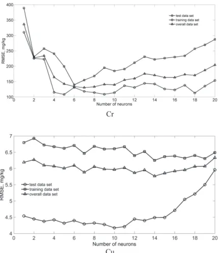
Results of the network structure selection (number of neurons in the hidden layer) are shown in figure 2. The following number of hidden neurons was selected: 6 for Cr and 10 for Cu.
Cr
Cu
FIGURE 2. Root mean square error (RMSE) of a neural network (MPL)
for test, training and overall data under different number of neurons in the hidden layer for Cr and Cu
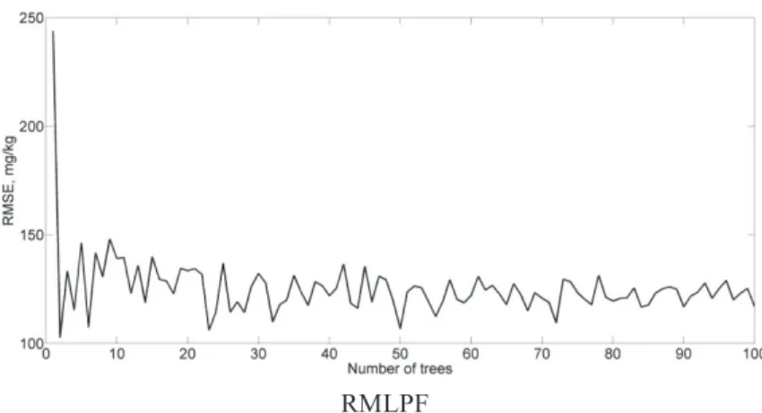
Fig. 3, 4 shows the dependencies of RMSE on the number of trees for the RF and RMLPF models. It can be seen that starting from about 20 trees the error varies around a certain constant value. With an increase of the number of trees, the fluctuations decrease slightly. This is true for both modeled elements.
RMLPF
FIGURE 3. Dependence of the RMSE index on the number of trees for the RF and RMLPF models for predicting chromium concentration
The accuracy assessment indices of predicted concentrations are shown in Table 2. TABLE 2. Accuracy assessment indices of predicted concentrations, mg/kg.
Method Index Cu Cr MLP MAE 3.73 70.3 RF MAE 2.81 95.6 RMLPF MAE 2.95 68.3 MLP RMSE 4.17 140 RF RMSE 3.37 169 RMLPF RMSE 3.36 117
As can be seen from Table 2, generally the RFMLP model showed the smallest errors. The improvement of the MAE index relatively the RF model was 29% for Cr, but for Cu MAE was almost 5% more. According to the RMSE index, the improvement was 31% for Cr. For Cu both errors were the same. The artificial neural network (MLP) also turned out to be more accurate than the results of RF for anomalous Cr (26% for MAE and 17% for RMSE). And on the contrary in case of conditionally normally distributed copper, RF was about 10% more precisely than MLP for both indices.
CONCLUSION
A study on the distribution of chromium and copper concentrations in the surface layer of soil at the urbanized terrain of the Tarko-Sale, Yamalo-Nenets Autonomous Okrug, Russia was conducted. A comparison was made for the machine learning methods: artificial neural networks, random forest, and an approach was proposed in which a multilayer perceptron, a random perceptron forest, was used as a classifier (tree). The new approach allowed to increase the accuracy of predicting the spatial distribution of the impurity, which had spots of anomalously high concentration in the upper soil layer. The increase in accuracy was 29% for the MAE index and 31% for the RMSE. A random forest based on regression in this case showed the worst accuracy. However, in simulating a normally distributed impurity, approaches based on RF algorithms have surpassed artificial neural networks.
In general, both models used for modeling have shown their effectiveness and versatility and are suitable for predicting the spatial distribution of impurities in environmental studies.
REFERENCES
1. A. J. Shepherd, Second-Order Methods for Neural Networks: Fast and Reliable Training Methods for Multi-Layer Perceptrons, Springer-Verlag, p 145 (1997).
3. J. Kukkonen, L. Partanen, A. Karppinen, J. Ruuskanen, H. Junninen, M. Kolehmainen, H. Niska, S. Dorling, T. Chatterton, R. Foxall, G. Cawley, Extensive evaluation of neural network models for the prediction of NO2 and PM10 concentrations, compared with deterministic modelling system and measurements in central Helsinki,
Atmos Environ 37(32): 4539–4550 (2003).
4. D. Jiang, Y. Zhang, X. Hu, Y. Zeng, J. Tan, D. Shao, Progress in Developing an ANN Model for Air Pollution Index Forecast, Atmos. Environ. 38: 7055–7064 (2004).
5. M. Bell, A. S. Bergantino, M. Catalano, F. Galatioto, Prediction of air pollution peaks generated by urban transport networks, Working papers SIET 2015 (2015).
6. S. V. Kottur, S. S. Mantha, An Integrated Model using Artificial Neural Network (ANN) and Kriging for Forecasting Air Pollutants using Meteorological Data, International Journal of Advanced Research in Computer and Communication Engineering. Vol. 4, Issue 1. 146–152 (2015).
7. A. De Souza, F. Aristones, F. V. Goncalves, Modeling of Surface and Weather Effects Ozone Concentration Using Neural Networks in West Center of Brazil, Climatology & Weather Forecasting. Volume 3. Issue 1. 123 (2015).
8. X. Feng, Q. Li, Y. Zhu, J. Hou, L. Jin, J. Wang, Artificial neural networks forecasting of PM2.5 pollution using air mass trajectory based geographic model and wavelet transformation, Atmospheric Environment 107 (2015) 118–128 (2015).
9. I. Anagu, J. Ingwersen, J. Utermann, T. Streck Estimation of heavy metal sorption in German soils using artificial neural networks, Geoderma, 152, 104–112 (2009).
10. Y. Li, C. Li, J.-J. Tao, L.-D. Wang, Study on Spatial Distribution of Soil Heavy Metals in Huizhou City Based on BP--ANN Modeling and GIS, Procedia Environmental Sciences 10. 1953–1960 (2011).
11. O. S. Hilko, S. P. Kundas, I. A. Gishkeluk, Radionuclides migration modelling using artificial neural networks and parallel computing, European water. 39. 3–13 (2012).
12. A. Falamaki, Artificial neural network application for predicting soil distribution coefficient of nickel, Journal of Environmental Radioactivity. 115. 6–12 (2013).
13. D. A. Tarasov, A. G. Buevich, A. P. Sergeev, A.V. Shichkin, High Variation Topsoil Pollution Forecasting in the Russian Subarctic: Using Artificial Neural Networks Combined with Residual Kriging, Applied Geochemistry, doi.org/10.1016/j.apgeochem.2017.07.0070, (2017) In Press.
14. L. Breiman, Random forests, Mach. Learn. 45, 5–32 (2001).
15. J. H. Friedman, J. J. Meulman, Multiple additive regression trees with applica-tion in epidemiology, Stat. Med.
22, 1365–1381 (2003).
16. R. L. Lawrence, S. D. Wood, R. L. Sheley, Mapping invasive plants using hyper-spectral imagery and Breiman Cutler classifications (Random Forest), Remote Sens. Environ. 100, 356–362 (2006).
17. R. Pouteau, S. Rambal, J.-P. Ratte, F. Gogé, R. Joffre, T. Winkel, Downscaling MODIS-derived maps using GIS and boosted regression trees: the case of frost occurrence over the arid Andean highlands of Bolivia, Remote Sens. Environ.115, 117–129 (2011).
18. J. Peters, N. Verhoest, R. Samson, P. Boeckx, B. De Baets, Wetland vegetation distribution modelling for the identification of constraining environmental variables, Landsc. Ecol. 23, 1049–1065 (2008).
19. J. T. Froeschke, B. F. Froeschke, Spatiotemporal predictive model based on environmental factors for juvenile spotted seatrout in Texas estuaries using boosted regression trees, Fish. Res. 111, 131–138 (2011).
20. D. C. Carslaw, P. J. Taylor, Analysis of air pollution data at a mixed source location using boosted regression trees, Atmos. Environ. 43, 3563–3570 (2009).
21. R. Grimm, T. Behrens, M. Märker, H. Elsenbeer, Soil organic carbon concentrations and stocks on Barro Colorado Island-digital soil mapping using Random Forests analysis, Geoderma 146, 102–113 (2008).
22. M. P. Martin, M. Wattenbach, P. Smith, J. Meersmans, C. Jolivet, L. Boulonne, D. Arrouays, Spatial distribution of soil organic carbon stocks in France, Biogeosciences 8, 1053–1065 (2011).
23. K. Sreenivas, G. Sujatha, K. Sudhir, D. V. Kiran, M. Fyzee, T. Ravisankar, V. Dadhwal, Spatial assessment of soil organic carbon density through random forests based imputation, J. Indian Soc. Remote Sen. 42, 577–587 (2014).
24. M. Wiesmeier, F. Barthold, P. Spörlein, U.Geuß, E. Hangen, A. Reischl, B. Schilling, G. Angst, M. von Lützow,
I. Kögel-Knabner Estimation of total organic carbon storage and its driving factors in soils of Bavaria (southeast Germany), Geoderma Reg. 1, 67–78 (2014).
25. K. Were, D. T. Bui, O. B. Dick, B. R. Singh, A comparative assessment of support vector regression, artificial neural networks, and random forests for predictingand mapping soil organic carbon stocks across an Afromontane landscape, Ecological Indicators. 52, 394–403 (2015).
26. Guo Peng-Tao, Li Mao-Fen, Luoa Wei, Tang Qun-Feng, Liu Zhi-Wei, Lin Zhao-Mu, Digital mapping of soil organic matter for rubber plantation at regional scale: An application of random forest plus residuals kriging approach, Geoderma. 237–238, 49–59 (2015).
27. Ren-Min Yanga, Gan-Lin Zhanga, Feng Liua, Yuan-Yuan Lua, Fan Yanga, Fei Yanga, Min Yanga, Yu-Guo Zhaoa, De-Cheng Li, Comparison of boosted regression tree and random forest models formapping topsoil organic carbon concentration in an alpine ecosystem, Ecological Indicators. 60, 870–878 (2016).