COMPARING ACCUARCIES OF SPATIAL INTERPOLATION METHODS ON 1-MINUTE GROUND MAGNETOMETER READINGS
A Thesis
Submitted to the Graduate Faculty of the
North Dakota State University of Agriculture and Applied Science
By
Kathryn Marie Campbell
In Partial Fulfillment of the Requirements for the Degree of
MASTER OF SCIENCE
Major Department: Statistics
Option:
[Name of Degree option. This is optional.]
May 2017
North Dakota State University
Graduate School
TitleComparing Accuracies of Spatial Interpolation Methods on 1-Minute Ground Magnetometer Readings
By
Kathryn Marie Campbell
The Supervisory Committee certifies that this disquisition complies with North Dakota State University’s regulations and meets the accepted standards for the degree of
MASTER OF SCIENCE SUPERVISORY COMMITTEE:
Dr. Seung Won Hyun Chair Dr. Rhonda Magel Dr. Yue Ge Approved: 06/12/2017 Dr. Rhonda Magel
ABSTRACT
Geomagnetic disturbances caused by external solar events can create geomagnetically induced currents (GIC) throughout conducting networks of Earth’s surface. GIC can cause disruption that scales from minor to catastrophic. However, systems can implement preemptive measure to mitigate the effects of GICs with the use of GIC forecasting. Accurate forecasting is dependent on accurate modeling of Earth’s geomagnetic field. Unfortunately, it is not currently possible to have a measurement at every point of Earth’s field. Spatial interpolation methods can be implemented to fill in for the unmeasured space. The performances of two spatial interpolation methods, Inverse Distance Weighting and Kriging, are assessed to determine which better predicts the unmeasured space. Error testing shows both methods to be comparable, with the caveat of Kriging having a tighter precision on predictions.
ACKNOWLEDGEMENTS
I would first like the thank the members of my committee for their time and insight provided. I would also like to thank my family and friends for their constant encouragement throughout my studies at North Dakota State University. Finally, I must express gratitude to my parents and my partner Jacob Lambeth for their unwavering support during my years of study. Thank you.
TABLE OF CONTENTS
ABSTRACT ... iii
ACKNOWLEDGEMENTS ... iv
LIST OF TABLES ... vii
LIST OF FIGURES ... viii
LIST OF APPENDIX TABLES ... ix
LIST OF APPENDIX Code Breifs ... x
1. INTRODUCTION ... 1
2. LITERATURE REVIEW ... 5
2.1. Inverse Distance Weighting (IDW) ... 5
2.1.1. Introduction and Theory ... 5
2.1.2. Correlation Addition to Weighting Function ... 5
2.2. Kriging ... 7
2.2.1. Introduction and Theory ... 7
2.2.2. Ordinary Kriging ... 7 2.2.3. Semivariogram ... 8 2.2.4. Spatial-Temporal Kriging ... 10 3. RESEARCH METHODS ... 13 3.1. Data Description ... 13 3.1.1. Description ... 13
3.1.2. Interpolation: Filling in Missing Data ... 15
3.1.3. Exploration ... 15
3.2. Error Testing ... 21
4. REAL DATA ANALYSIS ... 22
4.1.1. Correlation Analysis ... 22
4.1.2. Real Data Interpolation... 26
4.2. Kriging ... 36 4.2.1. Variogram Analysis ... 36 4.2.2. Interpolation ... 38 5. METHOD COMPARISONS ... 46 6. CONCLUSIONS/DISCUSSIONS ... 51 REFERENCES ... 53 APPENDIX A: Tables ... 55
LIST OF TABLES
Table Page
3.1: Descriptive Statistics of 1-minute ground magnetic readings ... 19
3.2: Descriptive Statistics of Transformed 1-minute Ground Readings ... 20
4.1: IDW Error Rates per Observatory: World Group ... 28
4.2: IDW Error Rates per Observatory: North Group... 29
4.3: IDW Average Error Rates: All Days ... 33
4.4: IDW Average Error Rates: Storm Days ... 33
4.5: IDW Average Error Rates: Calm Days ... 33
4.6: IDW T-Tests Storm vs Calm: Means ... 34
4.7: IDW T-Tests Results for Average Standard Deviations from Observatories ... 35
4.8: Kriging Error Rates per Observatory: World ... 39
4.9: Kriging Error Rates per observatory: North Group ... 42
4.10: Kriging Average Error Rates: All Days ... 44
4.11: Kriging Average Error Rates: Storm Days ... 44
4.12: Kriging Average Error Rates: Calm Days ... 44
4.13: Kriging T-Tests Storm vs Calm: Means ... 45
4.14: Kriging T-Tests Results for Standard Deviations ... 45
5.1: Descriptive Statistics of a Model’s Accuracy: Across all Observatories for All Days ... 46
5.2: T-Tests Interpolation Method’s Means... 47
5.3: T-Tests Interpolation Method’s Standard Deviations ... 48
5.4: Descriptive Statistics of a Model’s Accuracy: Storm Days ... 49
5.5: Method Comparisons Storm Days: Means ... 49
LIST OF FIGURES
Figure Page
2.1: Semivariogram model parameters. ... 9
2.2: A selection of permissible semivariogram models: ... 10
3.1: Observatory Locations (South, 2011) ... 14
3.2: Average Magnetic Reading per Day ... 16
3.3: Average Magnetic Field per Observatory: World ... 17
3.4: Average Magnetic Field per Observatory: North ... 17
3.5: Histograms of 1-minute Ground Readings ... 18
3.6: Histograms of transformed 1-minute Ground Readings ... 20
4.1: Correlation Coefficients for Observatory pairs: World ... 23
4.2: Correlation Coefficients for Observatory pairs: North ... 24
4.3: Interdependency Plot: World ... 25
4.4: Interdependency Plot: North ... 25
4.5: IDW Average Daily Error Rate per Day: World ... 31
4.6: IDW Average Daily Error Rate per Day: North ... 32
4.7: Variograms: World ... 36
4.8: Variograms: North ... 38
4.9: Kriging Average Daily Error Rate per Observatory: World... 40
LIST OF APPENDIX TABLES
Table Page
A1: Correlation Coefficients: World Group ... 55 A2: Correlation Coefficients: North Group ... 56
LIST OF APPENDIX CODE BREIFS
Code Page
B1: IDW ... 57 B2: Kriging ... 60
1.INTRODUCTION
Earth is enveloped by a geomagnetic field created by several sources, both internal and external to the planet. Multipole expansions are used to study the field. Assumed theory is that the field is made by the superposition of various fields from a series of poles found at the Earth’ center. Currently there is no recorded monopole, therefore the expansion begins with the known two, North and South poles or the dipole. Subsequent poles are then layered upon the previous. The source of the poles is found within the Earth, namely electric currents within the molten core. These internal sources are arguably the greatest influence on the creation and behavior of the field (McPherron, 2010).
The Earth’s field is measured by magnetometers scattered about the globe (Gjerloev, 2012). Magnetometers measure the strength and direction of local magnetic fields. They can measure fields on the Earth’s surface along with fields out towards space C.F Gauss (1832) developed one of the simpler magnetometers. A bar magnet is suspended by a gold fiber. The oscillations of the magnet are measured to find the surrounding field’s strength (Magnetometer, 2011). It is assumed from the multipole description of the Earth’s field “that the effects of the higher-order poles decrease more rapidly with distance than lower order poles” (McPherron, 2010).
Observations of the Earth’s fields have shown that it changes continuously with time. An example of this is the reversal of the dipole, which occur roughly between every 300,000 and 1,000,000 years. These fluctuations can be caused by natural elements of the internal forces or by external geomagnetic disturbances (GMDs). GMDs are caused by events on the sun, such as solar flares or coronal holes, reaching and interacting with Earth geomagnetic field. This interaction creates geomagnetically induced currents (GICs). GICs can disrupt conducting networks and
shortwave radio transmissions, increase corrosion in pipelines, create anomalies in communication satellites, and in extreme instances have catastrophic effects (McPherron, 2010). An example of the latter is the geomagnetic storm in March of 1989. A particularly strong GMD caused the Hydro-Quebec electrical system to fail for approximately nine hours. This left 6 million individuals without power (Boteler, 2003). Countries around the globe have taken steps to alleviate the effects of the GMDs. An example of this is the Space Disturbance Forecast Center in Boulder, Colorado. This center monitors the Sun and calculates predictions for GMDs and space weather (McPherron, 2010).
However, simply predicting GMDs does not lead to directly predicting the behavior of GICs; and adequate forecasting is required for systems to mitigate the effects of the GMDs by preemptively blocking or limiting the flow of GICs (Boteler, 2003). A key component of GIC modeling is a measurement of the Earth’s magnetic field. (Kazerooni, 2015). Unfortunately, magnetometer data is sparsely spread across the Earth’s surface. Spatial interpolation can be used estimate the magnetic field at non-measured locations. One of the more popular magnetic field models, The World Magnetic Model (WMM), “provides the complete geometry of the [magnetic] field” (Chulliat, 2015). Nevertheless, the WMM is limited by excluding GMD’s, and is only updated in five year intervals. It can be argued that there is a need for a spatial interpolation model that includes GMDs and can be quickly updated, to allowed for more accurate GIC forecasting.
One such model is proposed in M. Kazerooni (2015). A two-dimensional inverse distance weighting (IDW) function is used to model these external disturbances. This paper included a manipulation to the weight function to include the interdependences of magnetometer observatories via correlation analysis. The paper used real data from 21 irregularly spaces magnetometer observatories scattered across North America, and also measured interdependencies
within observatory pairs. Those interdependencies are then included in the IDW function in the hope it will increase performance. This new model boasted an accuracy of nearly 80% for predicated magnetometer reading against actual recorded values (Kazerooni, 2015).
Another spatial interpolation method, Kriging, has also been implemented in relation to measuring geomagnetic fields. Hao (2012) cross-validated accuracy of two-dimensional Kriging (without a temporal effect) against other methods for magnetic survey data. The paper implemented a gridding pattern to sample local regional geomagnetic field in Northwest China with 3131 measured points. Kriging’s accuracy was compared against serval other methods such as, IDW, Natural Neighbor, Polynomial Fitting, and others. In Hao (2012) Kriging significantly outperformed its counterparts in “terms of small-scale magnetic data interpolation.” However, Hao (2012) includes only locally measured and equally spaced gridded sampled points. Therefore, it is unknown if Kriging performance increases or decreases when extended to a global scale and/or with irregularly spaced data. An interest of this thesis is implementing Kriging in those untested situations and measuring its performance.
The focus of this thesis is replicating the proposed two-dimensional IDW model from Kazerooni (2015), and comparing it against a Kriging interpolation model that includes a temporal element. These methods are chosen because of previous interest in them with regards to geomagnetic interpolation. Other methods were considered, such as Natural Neighbor, however computational constraints limited this thesis to only consider Kriging and IDW. Cross validation is applied to determine which method better depicts the geomagnetic field.
While a model’s accuracy is assessed, there is a particular interest to see if the model preforms well during solar activity. The year of 2012 had several space weather events that significantly affected Earth’s geomagnetic field. January 19th, 2012 saw the year’s first coronal
mass ejection (CME). It made landfall early morning of the 22nd and caused minor disturbances (Phillips, 2012). The largest solar flare since May 2005 erupted on January 23rd, 2012 accompanied by a CME. The arrival of the CME was on the 24th and caused minor level geomagnetic storm (Phillips, 2012). On March 6th, 2012, a region of the Sun erupted with two solar flares within an hour of each other. These solar flares were accompanied by two CMEs, both of which were directed towards the Earth. The activity on March 6th struck an Earth that was already experiencing a moderate geomagnetic storm caused by activity on March 2nd (Fox, 2012). The previous are a few examples of the solar activities during 2012. However, all recorded geomagnetic storm days in 2012 will be used to measure a model’s precision during turbulent space weather.
The theory and background for Kriging and IDW is provided in Section2. Section 3 contains the preliminary data exploration and the required transformation for interpolation implementation. Both interpolation methods are performed on the same data, and their respective performances are found in Section 4. Section 5 contains the method comparisons, and the thesis finishes with the conclusions and thoughts for future research in Section 6.
2.LITERATURE REVIEW
2.1.Inverse Distance Weighting (IDW)
2.1.1.Introduction and Theory
Shepard (1968) proposed a two-dimensional spatial interpolation function. From a data set of known locations 𝑥𝑖 with recorded values 𝑧𝑖 for 𝑖 = 1,2, … , 𝑁, an interpolated value z(x) at
unmeasured point x is calculated using the following function:
𝑧(𝑥) = ∑ 𝑤𝑖(𝑥)𝑧𝑖 ∑𝑁𝑖=1𝑤𝑖(𝑥) 𝑁
𝑖=1
The influence between points is measured by the weighting function 𝑤𝑖. The larger the weight the
greater influence. Weights decrease as the distance increases between 𝑥 and 𝑥𝑖. This aspect puts more significance on known points at a more immediate distance with respect to 𝑥. One of the simplest weighting functions defined in Shepard (1968) is
𝑤𝑖(𝑥) = 1 𝑑(𝑥, 𝑥𝑖)𝑝,
where 𝑑(𝑥, 𝑥𝑖) is the distance between 𝑥 and 𝑥𝑖, raised to the power parameter 𝑝 > 0. An interesting caveat of IDW is that its weighting function can be manipulated depending on the interpolation circumstances and goals of the experimenter. An example of this is proposed in Kazerooni (2015) which is discussed in the next section.
2.1.2.Correlation Addition to Weighting Function
Kazerooni (2015) suggests that the magnetic fields around the observatories may have unforeseen dependencies with other observatories. These dependencies are folded into the study’s IDW weighting function with the creation and addition of an indicator variable 𝑐(𝑥, 𝑥𝑖). The
methodology behind this new variable from Kazerooni (2015) is found in the following paragraphs. 𝑤𝑖(𝑥) = 𝑐(𝑥, 𝑥𝑖) 𝑑(𝑥, 𝑥𝑖) 𝑐(𝑥, 𝑥𝑖) = {1 𝑖𝑓 𝑥 𝑎𝑛𝑑 𝑥𝑖𝑎𝑟𝑒 𝑑𝑒𝑝𝑒𝑛𝑑𝑎𝑛𝑡 0 𝑜𝑡ℎ𝑒𝑟𝑤𝑖𝑠𝑒
𝑐(𝑥, 𝑥𝑖) indicates the dependency between locations, and the dependency is calculated through
correlation analysis between the known points. To find the dependency within pairs, Pearson’s correlation coefficient is calculated across entire time interval. It’s defined as:
𝜌𝑥𝑥𝑖 =
𝑐𝑜𝑣(𝑥, 𝑥𝑖) 𝜎𝑥∗ 𝜎𝑥𝑖
with 𝑥 and 𝑥𝑖 being a single observatory respectfully, 𝑐𝑜𝑣(𝑥, 𝑥𝑖) the covariance between the observatories, and finally σ as the standard deviation for a single observatory. The probability of dependency between observatory pairs is calculated from
𝑃(𝑥1, 𝑥2) = ∑ 𝑐𝑜𝑒(𝑥1,𝑥2)𝑗 𝐷
𝑗=1
𝐷 ,
where D is the total number of days and an indication for correlation strength for each 𝑗𝑡ℎ day is defined as:
𝑐𝑜𝑒(𝑥1, 𝑥2)𝑗 = {1 𝑖𝑓 𝑐𝑜𝑟𝑟𝑒𝑙𝑎𝑡𝑖𝑜𝑛 𝑐𝑜𝑒𝑓𝑖𝑐𝑖𝑒𝑛𝑡 𝑖𝑠 ≥ 0.5 0 𝑜𝑡ℎ𝑒𝑟𝑤𝑖𝑠𝑒
2.2.Kriging
2.2.1.Introduction and Theory
Kriging was first proposed in Krige (1951) and later perfected in Mathenm (1960). Using existing data, Kriging interpolates missing value data by providing the best linear unbiased prediction at unmeasured locations. It utilizes “the spatial positions of points to be interpolated and neighboring observations points” (Hao, 2012), the spatial relationships between neighboring points, and the spatial distribution of the data. Depending on the properties of the field being interpolated, different methods of Kriging can be applied. Regarding this thesis Ordinary Kriging is implemented for estimating Earth’s geomagnetic field.
2.2.2.Ordinary Kriging
The following information is obtained from Hao (2012. In a sample of size N on an area of research, 𝑖𝑡ℎ sampled point is denoted by 𝑍
𝑖(𝑥, 𝑥𝑖) where x is the interpolated point and 𝑥𝑖 is a
measured point, with 𝑖 = 1,2 … . , 𝑁 for all sampled locations. The interpolated point, denoted 𝑍0
is calculated from the weighted sum of the sampled values.
𝑍0 = ∑𝑚𝑖=1𝜆𝑖𝑍𝑖(𝑥, 𝑥𝑖), where 𝜆𝑖 is the weighted coefficient of 𝑖𝑡ℎ sampled values.
Ordinary Kriging has the following assumptions. First the mean, or expected value of points 𝑍𝑖(𝑥, 𝑥𝑖), of the research field exists and is equal to a constant 𝑚:
𝐸(𝑍(𝑥, 𝑥𝑖)) = 𝑚.
Second, covariance functions of the points 𝑍𝑖𝑎𝑛𝑑 𝑍𝑖∗ exist. This implies they are only dependent
on spatial lag distance h and not their positions.
Minimizing the variance of the estimations results in the following: ∑ ∑ 𝜆𝑖𝛾(ℎ𝑖 − ℎ𝑗) + 𝜇 = 𝛾(ℎ0− ℎ𝑖) 𝑚 𝑗=1 𝑚 𝑖=1
where 𝑖, 𝑗 = 1,2, . . . , 𝑚, 𝜇 is the Lagrange constant, 𝛾(ℎ𝑖− ℎ𝑗) and 𝛾(ℎ0− ℎ𝑗) are the
semivariograms between the sampled points and given point and interpolated point respectfully. The theory and importance of the semivariogram for Kriging is found in the following section. 2.2.3.Semivariogram
A semivariogram is the measure of spatial correlation, i.e. how data is correlated with distance. It’s defined as:
𝛾(ℎ) = ( 1
2𝑁ℎ)(∑ [𝑍𝑖+ℎ − 𝑍𝑖] 2) 𝑁ℎ
𝑖=1 ,
where 𝑁ℎis the total number of sampled pairs whose distance is equal to h (Hao, 2012). Usually, the Euclidean distance is used. However, this thesis implemented the great circle distance instead. Where the distance d is found by
𝑑 = 𝑟Δ𝜎, Δ𝜎 = 2arcsin (√sin2(Δ𝜙
2 ) + cos(𝜙1) ∗ cos(𝜙2) ∗ sin 2(Δ𝜆
2),
where 𝜙1, 𝜆1, and 𝜙2, 𝜆2are the geographical latitude and longitude of the two observations, along
with Δ𝜙 and Δ𝜆 as their absolute differences (Rios, 1975). This distance formula is chosen due to the expansive sampled areas that are either the entire North American continent or the Globe.
𝑍𝑖+ℎ and 𝑍𝑖 are values of the observatory pair whose distance is equal to h.
Variogram analysis is done before the actual Kriging. The goal is to find an adequate semivariogram model that best estimates the underlying spatial correlation in each research area. An experimental semivariogram is constructed from the sampled data. First a set separation distance (h) is chosen. Then the average, 𝛾(ℎ), for each 𝑁ℎ of pairs’ 𝑍𝑖 squared difference is
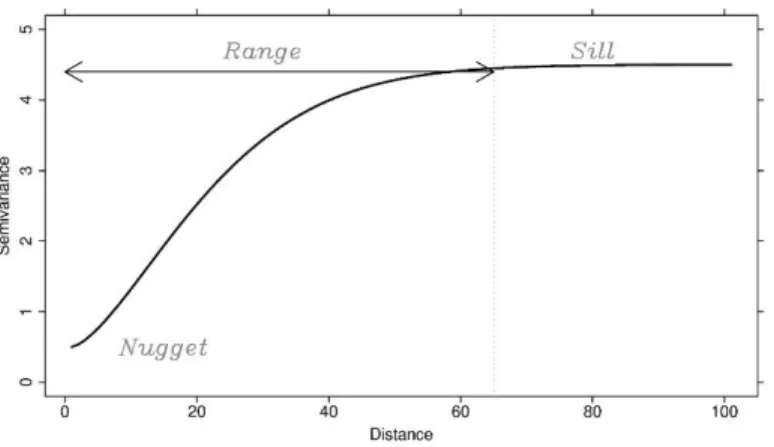
calculated. The experimental semivariogram is then plotted and used to fit a model. This is derived by a combination of model selection and fitting parameters (Hao, 2012). Parameters of the semivariogram are, sill, range, and nugget. Sill measures variance as distance between points increases. The distance that points become uncorrelated is denoted by the range. Nugget reports measurement error or noise within the data. Figure 2.1 is a graphical display of these parameters. Common theoretical semivariogram models are presented in Figure 2.2.
Figure 2.1: Semivariogram model parameters.
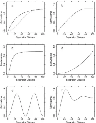
Figure 2.2: A selection of permissible semivariogram models:
(A) Powered Exponential model (i) Broken line with power (ω)=2, equivalent to a Gaussian model. (ii) Solid line with ω=1. (B) Spherical model. (C) Rational Quadratic model. (D) Power model. (E) Cosine (hole effect) model. (F) Dampened Hole model. (Spadavecchia, n.d.) 2.2.4.Spatial-Temporal Kriging
Arguably most spatial measurements have some temporal influence. Examples include the periodic changing seasons, sudden weather or geological events, catastrophic actions of mankind, and more. All could be influential on the behavior of a spatial plane. Including temporal information should, in theory, improve any interpolation or prediction. An interesting aspect of Kriging is its ability to interpolate on a spatial-temporal plane. The following are a few methods of incorporating this information to improve interpolation.
Because the semivariogram is a function of the distance between pairs it is easily extended into higher dimensions. Using this property time can be considered as a third orthogonal dimension, elevating the interpolated spatial plane into a spatial-temporal plane. The only caveat
of this manipulation is that interval of time needs to be rescaled to fit with the physical spatial dimension (Benedikt Graler, 2011). A suggestion for geomagnetic readings, the 1-mintue intervals can be rescaled into radians. A single day would be equal to one full rotation around a unit circle or 2𝜋. Therefore, the first minute of the first day is 0, and the last minute of the first day is 2𝜋.
Subsequent days are treated as multiple rotations. For example, the last minute of the second day has the value 4𝜋. The physical distance between pairs is still calculated by the great circle distances with the output formula in radians instead of miles. First the physical distance between pairs is calculated, and then their distance in time. This results in the following distance formula:
𝑑3(𝑥, 𝑡𝑋, 𝑦, 𝑡𝑦) = √(𝑑2(𝑥, 𝑦))2+ (𝑡
𝑥− 𝑡𝑦) 2
,
with x and y as individual observatories, whose longitude and latitude values in degrees, and 𝑡𝑥, 𝑡𝑦
as the specific point in time for each observatory. Finally, 𝑑2 is the great circle distance between x and y. This method rakes full advantage of the temporal information and is considered a full spatial-temporal model. However, it can become computationally heavy, as the combinations between different points of time at a physical location can increase very quickly with the addition of more sampled locations.
Another method is Daily Evolving Semivariogram. The empirical semivariogram is calculated with information from a single day only. The fitted model’s parameters are then calculated from the daily semivariogram and previous days parameter estimates with “exponentially decaying influence” (Benedikt Graler, 2011). Even though Kriging interpolation is still performed per time instances, the evolving semivariogram somewhat include the temporal information (Benedikt Graler, 2011). As with the previous method, calculating the evolving semivariogram for every time slices, in the context of this thesis a new semivariogram per minute, is computationally heavy when using a large interval of time. The evolving semivariogram and the
3-dimensional approach proved to be too difficult for the capabilities of this thesis and a third method is sought after.
Assuming a constant spatial (but not temporal) structure throughout the interval allows for the creation of a pooled semivariogram. The pooled semivariogram is created by averaging the empirical variograms per time slice. Then interpolation uses the same variogram per instance of time (Benedikt Graler, 2011). Of the methods mentioned, this is the least computationally intensive and the one implemented in this thesis.
3.RESEARCH METHODS
3.1.Data Description
3.1.1.Description
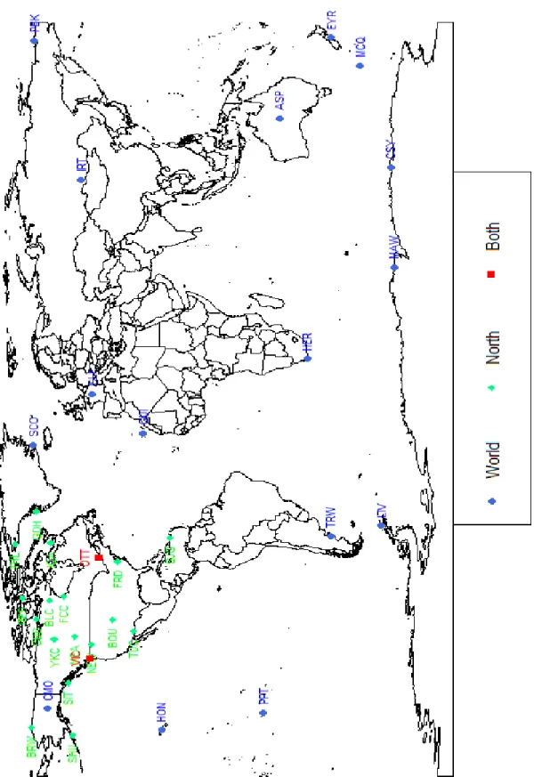
The data analyzed was collected from the SuperMAG (http://supermag.jhuapl.edu/) website. 1-minute ground, i.e., readings at ground level per minute, magnetometer data (Gjerloev, 2012), from January 1st, 2012 to December 31st, 2012, is collected from 35 observatories. Observatory locations are displayed in Figure 3.1. The 35 observatories are split into two groups for analysis. The first group are spread across the globe in a pseudo grid like pattern. The second groups is made up of 19 of the 35 observatories and are located only on in the North American continent. Some observatories appear in both groups. Analysis is performed on the two groupings separately, with the North American and global locations subsequently referred to as North and World respectively. The magnetic readings are in three directions, North, East, and vertical. The vertical direction does not affect power systems and was not included. Analysis on the North and East directions can be performed separately (Kazerooni, 2015); but due to time and computational limitations only the North direction is presented in this thesis. However, the East direction can be substituted in place of the North readings and analyzed with the same methods.
3.1.2.Interpolation: Filling in Missing Data
For various reasons observatories may have incomplete data for the whole time interval. The interpolation methods in this thesis are performed on a single minute and use the values from all recorded locations. Missing location can impact the interpolation. Kriging is especially susceptible to this as the removal of an observatory could drastically adjust the semivariogram for that minute. Before beginning the interpolation, the 1 minute ground magnetic data screened to fill in those missing data values. Using the minute increments, missing data is filled in with linear interpolation and extrapolation which is defined below:
𝑣0 = 𝑣1+ (𝑡0 − 𝑡1) (𝑣2−𝑣1 𝑡2−𝑡1),
The interpolated/extrapolated magnetic value is denoted by 𝑣0, with 𝑡0 as the corresponding
minute. 𝑣1, 𝑣2 are the recorded values of closest minutes 𝑡1, 𝑡2 on either side of 𝑣0. For example, assume the magnetometer failed to record a value on the 6th minute of the 1st day, but recorded values during the 5th and 7th minute. Those values are used to interpolate a magnetic reading for the 6th minute. This interpolation is only applied on observatories that originally contain magnetic values for at least 80% of the interval, a threshold that was arbitrarily set. Observatories that fail to meet this requirement are removed. Each spatial interpolation method is performed on a single time slice; in this instance, a single minute. Because of this, input is required from each sample location per minute.
3.1.3.Exploration
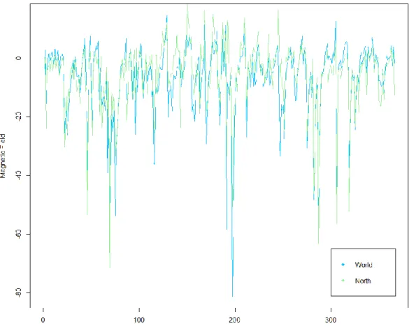
The average daily 1-minute ground magnetic readings across all observatories for each group is displayed in Figure 3.2. Of note, both groups appear to behave similarly. The large negative spikes correspond with recorded solar activity and appears to have affected both groups
equally. Most the magnetic readings appear to fall within [-20,0], which corresponds with days that have no recorded extreme space weather activities. This figure supports the idea that there is a temporal effect on the geomagnetic field.
Figure 3.2: Average Magnetic Reading per Day
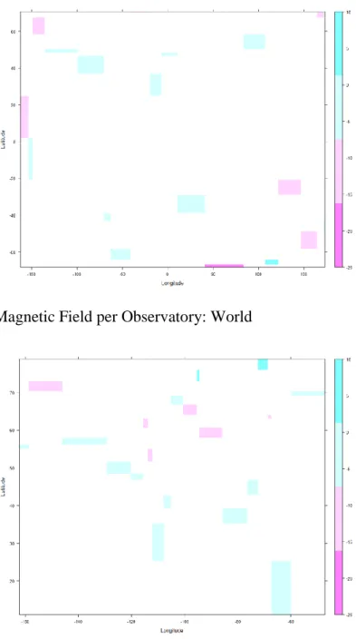
Recall from section 2.2.2 that Ordinary Kriging assumes a constant mean throughout the area of interest. This means that there should not be an obvious trend present in the recorded values. The average magnetic value per observatory is displayed in Figures 3.3 and 3.4. The bars on the right side of the graph measures the average ground magnetic reading. The values increase from negative to positive values via from the deep pink to bright cyan shades. These plots are used to see if there is an underlying trend present in the spatial plane. A display showing a steady color
change in a specific direction is an example of a trend. Through the samples are sparse and the play marked by white space, it can still be seen that there is not a distinct trend in either group. This allows Ordinary Kriging to be a viable interpolation method for the 1-minture ground magnetic readings.
Figure 3.3: Average Magnetic Field per Observatory: World
The Histograms presented in Figure 3.5 show that the magnetic ground data is approximately bell shaped however, the data is severely negatively skewed. However, the extreme outliers are not displayed in the histograms as the x axes has been adjusted. Table 3.1 contains descriptive statistics, including Pearson’s Skewness and Kurtosis coefficients, for the two observatory groups.
Table 3.1: Descriptive Statistics of 1-minute ground magnetic readings
Group Mean Median Standard Deviation Min Max Skewness Kurtosis
World -7.0331 -2.3 44.6786 -2401.3 672.6 -5.4134 95.9543
North -5.7158 -1.6 52.4348 -2791.4 96806 -4.1788 68.4511
While IDW has no assumptions for the samples data; Ordinary Kriging requires that the response variable be approximately normally distributed. Transformation provides the added benefits of suppressing outliers, and improving stationarity of the data. This thesis chose a Rank Order transformation (J. Wu, 2006). First all the data points 𝑛 are arranged in an increasing order
𝑧(1) ≤ 𝑧(2)≤ ⋯ ≤ 𝑧 (𝑛),
where 𝑧𝑟 is the 𝑟𝑡ℎordered 1-minute ground reading with 𝑟 = 1,2, … , 𝑛 , and 𝑛 is equal to the
total number magnetic readings in the data set. Therefore 𝑧(𝑟) is the 𝑟𝑡ℎ order statistic. The
standardized rank 𝑦(𝑟) of the sample is calculated
𝑦(𝑟)= 𝑟 𝑛 .
With the value of 𝑦(𝑟)falling within the interval of 1
𝑛 and 1 (J. Wu, 2006). This is done so that
the transformed data follows an approximately standard normal distribution.
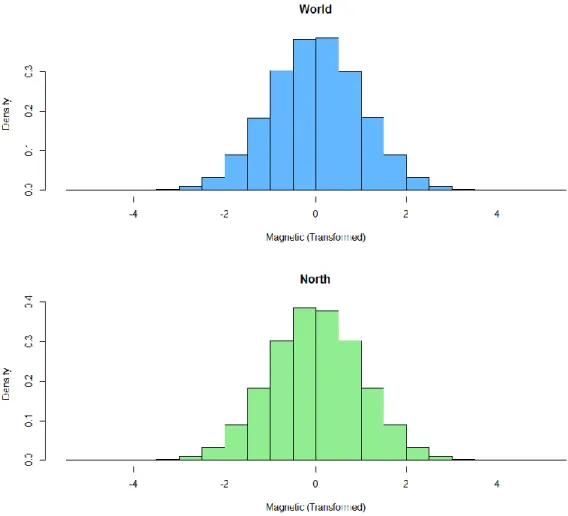
Figure 3.6 displays the transformed ground magnetic data. The transformation has addressed its skewness issue and the histograms now show a nearly symmetric bell-shaped distributions. Descriptive statistics for the newly transformed data are displayed in Table 3.2. The
transformed data now has an approximately normal distribution which closely resembles the standard normal. Spatial interpolation is then performed on the ranked values (J. Wu, 2006).
Figure 3.6: Histograms of transformed 1-minute Ground Readings
Table 3.2: Descriptive Statistics of Transformed 1-minute Ground Readings
Group Mean Median Standard
Deviation
Min Max Pearson’s Skewness
Pearson’s Kurtosis
World -3.7699e-07 -0.0044 0.9999 -5.3171 5.3171 -1.8471e-06 3.0000
3.2.Error Testing
N-1 Error testing is used to measure the performance of a method (Kazerooni, Use of Sparse Magnetometer Measurements for Geomagnetically Induced Current Model Validation, 2015). This method of performance testing creates a sub-set data set by removing a single location. The sub-set is then used to interpolate value at the removed location. Then the interpolated value is compared against the actual recorded value at that location. Methods that interpolate a value more closely to the actual reading are deemed to be more accurate than methods that have a larger discrepancy between predicted and actual values.
This was the method used in Kazerooni (2015). It seems pertinent to simply extend the comparison formula used previously to include Kriging. N denotes the total number of observatories in the data, and the “-1” occurs when a single observatory is removed from the data. This reduced data sub-set is then used to interpolate values at the removed observatory’s location. Performance is quantified by comparing the interpolated values against the actual magnetic field readings for that location. Recall from section 3.1.3 that the original 1-minute ground magnetic values are run though a rank order transformation. Those ranked values are used to interpolate at removed locations. The following error function is used in the comparison between the real transformed and interpolated values:
𝐸𝑟𝑟𝑜𝑟 = ||𝑈̂−𝑈||2 ||𝑈||2 ,
where 𝑈̂ and 𝑈 as vectors of the transformed recorded and interpolated values. ||. ||2is the Euclidean norm. This process is repeated across all observatory locations, days, and minutes for both the North American and World observatory groups.
4.REAL DATA ANALYSIS
4.1.IDW
4.1.1.Correlation Analysis
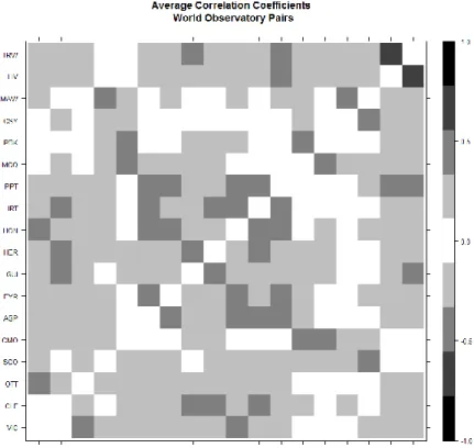
Before IDW is implemented, correlation analysis is preformed to find any underlying relationships between observatory pairs to include in the weighting function. Pearson’s Correlation Coefficient has a range of [-1, 1] with values near ±1 indicating a strong correlation, while values closer to 0 suggest a weak relationship. In Figures 4.1 and 4.2, the strength of the correlation between pairs is indicated by black for a strong, grey for moderate, and white no correlation. The axes are denoted by an observatory name; hence, a cell’s position indicates which pair is being compared. For example, in Figure 4.1, to find the correlation between VIC and OTT, start from VIC on the x-axis then find OTT on the y-axis, and check the cell where they intersect. In this instance, VIC and OTT have a moderate correlation. Note that cells with matching labels per axis, default to white. These matching pairs are found on the diagonal on the two figures.
Correlation coefficients for the World group are displayed in Figure 4.1. The strongest pair is TRW and VIC. A few pairs without a correlation are, VIC and CLF, GUI and SCO, and OTT and MCQ. The pair with the strongest correlation is TRW and LIV. PBK and CSY have the least number of correlated pairs. Remarkably, neither of them are isolated geographically from other observatories. Which can be seen in observatory map presented in Figure 3.1. Finding those listed observatories on the map shows that they are not isolated from other observatories by great distances. This could imply that distance is not the only indicator for influence between locations. Baring these two observatories, the other have numerous interdependencies, though they may not be strong in nature. Numeric values of the correlation coefficients are found in the Appendix.
Figure 4.1: Correlation Coefficients for Observatory pairs: World
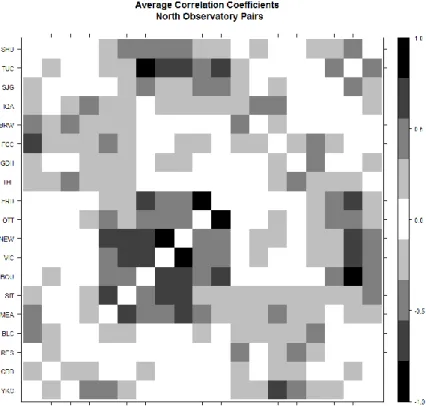
However, the observatories in the North group behave differently. From Figure 4.2 the strongest correlated observatory pairs are TUC and BOU, FRD and OTT, and NEW and VIC. This is two more pairs than that of the World group. On the other side of the scale RES appears to have the least interdependencies. It only has five non-zero coefficients, and of those none of them are strong. RES, like PBK and CSY in World, is not geographically isolated, on the contrary of the observatories is has the highest number of close neighbors. Unlike the World group, North has a larger amount on uncorrelated and strongly correlated observatory pairs. A possible explains for this is the closer proximity of the North observatories compared to the spread-out grid pattern found in World; as the influence of between location generally decreases as distance increases.
Figure 4.2: Correlation Coefficients for Observatory pairs: North
Figures 4.5 and 4.6 display the dependency across pairs for World and North groups respectively. The total number of combinations for observatories pairs is found using the follow formula:
(𝑁 2) =
𝑁! 2! (𝑁 − 2)! ,
where 𝑁 is the total number of observatories in the sample. N is equal to 18 and 19 for World and North respectfully. Recall from section 2.1.2 that observatories pairs are deemed dependency if they have a probability of dependency greater than or equal to 0.5. Figures 4.5 and 4.6 display those interdependencies. The observatories pair with interdependency are marked by darker cells.
Figure 4.3: Interdependency Plot: World
From Figure 4.5, 11 of 153 (7%) possible observatory pairs, in the World group, have some dependency with each other. 21 of 171 (12%) of possible North pairs show dependency in Figure 4.6. VIC, CSY, and OTT in World have no dependences with other observatories. In North, IQA, CBB, BLC, and GDH have not interdependencies. IDW’s modified weighting function uses the interdependencies to calculate the influence between points. Therefore, observatories that have no interdependences will be treated differently during interpolation than observatories with no interdependences. This is explored more in the following section.
4.1.2.Real Data Interpolation
Recall from Figure 4.5 that the observatories VIC, OTT, and CSY have no dependences with other locations. Therefore, IDW is unable interpolate a value at those locations. The reason for this is found in IDW’s weighting function. 𝑐(𝑥, 𝑥𝑖) returns 0 for all known pairs that include the independent observatories, reducing their influence on the interpolated location to 0. This effectively disregards the independent observatory from the rest of the group, as these three observatories do not have a discernable relationship between themselves and the rest. As such, their values cannot be interpolated; and similarly, these locations are not included in the interpolation for the remaining observatories.
Table 4.1 contains the summary statistics for the error testing for World. Observatories with “*” for values are ones that do not have interdependencies. In Figure 4.5, of note GUI and PBK have only a dependency with one other observatory, and in Table 4.1 have the largest ranges of error at 16.7538 and 24.6689 respectfully. Along with the highest ranges, GUI and PBK have two of the higher mean errors of 1.1140 and 1.0944 as well as the highest standard deviations of 1.3640 and 1.5320 respectfully. Conversely, ASP has the most dependent pairs at three and has the lowest mean error of 0.6202, along with the second to smallest range of 1.892
Like VIC, OTT, and CSY in World, North has four observatories (BLC, CBB, GDH, and IQA) without dependencies. BLC, CBB, GDH, and IQA, are disregarded during the interpolation for the remaining observatories. Table 4.2 displays the summary statistics for the error testing for North. Unlike World, Table 4.2 shows that North has little variation among the ranges of error per observatory. All the locations fall within in two units of each other. This could be explained from North’s higher amount of interdependences between observatories; as its interpolation included more information. The variation between the two groups is most evident in Figures 4.7 and 4.8; where World has significant spikes of error rates across the days in contrast to North more consistent error rates. Of note the larger spike in Figure 4.7 do correspond with dates that had significant solar activity.
Table 4.1: IDW Error Rates per Observatory: World Group
Observatory VIC CLF OTT SCO CMO ASP EYR GUI HER
Mean * 0.8285 * 0.9864 0.9211 0.6202 0.8178 1.1140 00.8673 Median * 0.7600 * 0.9614 0.8745 0.5952 0.7524 0.7937 0.7977 Std. Deviation * 0.4249 * 0.2329 0.2871 0.3237 0.4247 1.3640 0.4679 Min * 0.1155 * 0.4553 0.4295 0.0852 0.1152 0.1613 0.1264 Max * 3.0076 * 2.0714 2.2927 1.9780 2.9790 16.9151 3.0521 Range * 2.8921 * 1.6161 1.8632 1.8928 2.8638 16.7538 2.9257
Observatory HON IRT PPT MCQ PBK CSY MAW LIV TRW
Mean 0.6656 0.8534 0.7064 0.9137 1.0944 * 1.0437 0.8767 0.7339 Median 0.5988 0.7831 0.6373 0.8456 0.8776 * 0.9823 0.7872 0.6619 Std. Deviation 0.4427 0.4789 0.4551 0.3953 1.5320 * 0.3310 0.5177 0.3865 Min 0.0525 0.0791 0.0504 0.3531 0.3933 * 0.4830 0.1448 0.1335 Max 2.9934 3.6352 2.4298 3.6280 25.0622 * 2.7929 3.6964 2.1822 Range 2.9409 3.5561 2.3794 3.2749 24.6689 * 2.3099 3.5516 2.0487
Table 4.2: IDW Error Rates per Observatory: North Group
Observatory YKC CBB RES BLC MEA SIT BOU VIC NEW
Mean 0.7417 * 0.8857 * 0.7398 0.6155 0.3683 0.3899 0.3599 Median 0.7066 * 0.8683 * 0.7337 0.5967 0.3470 0.3802 0.3508 Std. Deviation 0.2531 * 0.2408 * 0.2139 0.2467 0.1792 0.1560 0.1441 Min 0.3502 * 0.1953 * 0.1664 0.0964 0.0757 0.0491 0.0543 Max 3.1050 * 1.5838 * 1.3092 2.6310 1.2519 1.4183 1.0810 Range 2.7457 * 1.3885 * 1.1428 2.5346 1.1762 1.3692 1.0267
Observatory OTT FRD THL GDH FCC BRW IQA SJG TUC SHU
Mean 0.5239 0.44174 0.8111 * 0.7725 0.9679 * 0.6885 0.4869 0.8189 Median 0.4877 0.3878 0.7933 * 0.7365 0.9325 * 0.6421 0.4579 0.8030 Std. Deviation 0.2725 0.2208 0.2117 * 0..2247 0.2754 * 0.3638 0.2265 0.3145 Min 0.1112 0.0595 0.2557 * 0.3661 0.4485 * 0.0622 0.0734 0.1191 Max 3.2185 1.4643 1.4572 * 1.6190 2.4219 * 1.8360 1.3855 1.9111 Range 3.1073 1.4048 1.2015 * 1.2529 1.9734 * 1.7738 1.3121 1.7920
In World and North, is appears that the average error for interpolation is at its lowest at observatories that have the most interdependences with other observatories in their respective groupings. These locations also exhibit less variability in error across the year, unlike observatories with little dependence on others. For example, in Figure 4.7 the largest spike found near day 100, is from observatory PBK. Which, along with the largest range of error, has the highest mean error, and standard deviation, and only one interdependency. On the other side of things, ASP has the lowest mean error rates, and the most interdependences at three. In Figure 4.7 ASP’s daily mean error is consistently between 0 and 2. Additionally, North has more interdependences overall than World.
Interestingly, IDW has a higher accuracy on stormy days’ verse calm ones. Tables 4.3 – 4.5 contain the average descriptive statistics per sample group. For World, it has an average error for is .8783 for calm days. But sees an over 20% drop in error for days that experienced space weather .6330. This trend is seen in the North group as well, with the error dropping from .6425 to .5494 for stormy days. Of note the model preforms objectively better for the North than the World one. This could be attributed to North’s higher number of interdependent observatories, along with their closer proximity with each other.
Table 4.3: IDW Average Error Rates: All Days
Group Avg. Mean Avg. Median Avg. Std Avg. Min Avg. Max Avg. Range
World 0.8570 0.8001 0.6654 0.0504 25.0622 25.0118
North 0.6392 0.6121 0.3111 0.0491 3.2185 3.1694
Table 4.4: IDW Average Error Rates: Storm Days
Group Avg. Mean Avg. Median Avg. Std Avg. Min Avg. Max Avg. Range
World 0.6330 0.4718 0.7504 0.0.0669 7.8321 7.7652
North 0.5494 0.4932 0.3255 0.0542 1.6158 1.5616
Table 4.5: IDW Average Error Rates: Calm Days
Group Avg. Mean Avg. Median Avg. Std Avg. Min Avg. Max Avg. Range
World 0.8783 0.8082 0.6605 0.0504 25.0622 25.0118
North 0.6425 0.6125 0.3101 0.0491 3.2185 3.1694
T-tests are implemented to check the validity of the above claims and are conducted within each group. Note that none of the following tests compare the sampled groups against each other; but rather, they are testing the behavior of the observatories within in a sampled group. The tests
use the means of the observatories within in group per weather type. Both tested groups sizes are under 30, and therefore the small sample T-tests is implemented. The results are found in Tables 4.6 and 4.7.
Table 4.6: IDW T-Tests Storm vs Calm: Means
Group Results
World
T Statistic P Value 95% CI for 𝝁𝑺𝒕𝒐𝒓𝒎− 𝝁𝑪𝒂𝒍𝒎 -2.4088 0.0268 (-0.4591, -0.0315)
North
T Statistic P Value 95% CI for 𝝁𝑺𝒕𝒐𝒓𝒎− 𝝁𝑪𝒂𝒍𝒎 -1.0902 0.2856 (-0.2685,0.0824)
When observing just the means, North does not appear to have a notable change in performance with a change in weather. On the other hand, the T-tests does confirm the suspicion that the performance does change significantly with the weather for World. In this case, the performance increases on recorded storm days. However, when looking at just standard deviations, there appears to not be a change in the methods performance’s variation across weather types for either group. T-tests are conducted on the average standard deviation per observatory for each sample group. I.E testing the average difference between observation locations in North, across the two weather types. The results are found in Table 4.7
Table 4.7: IDW T-Tests Results for Average Standard Deviations from Observatories
Group Results
World
T Statistic P Value 95% CI for 𝑺. 𝑫𝑺𝒕𝒐𝒓𝒎− 𝑺. 𝑫𝑪𝒂𝒍𝒎
-0.8534 0.4020 (-0.5271,0.2189)
North
T Statistic P Value 95% CI for 𝑺. 𝑫𝑺𝒕𝒐𝒓𝒎− 𝑺. 𝑫𝑪𝒂𝒍𝒎
4.2.Kriging
4.2.1.Variogram Analysis
The empirical semivariogram, calculated from the sample data, is used to define the fitted semivariogram that is used during Kriging. Figures 4.9 and 4.10 have World and North’s respective empirical and fitted semivariograms from the transformed 1-minute ground magnetic readings. The empirical semivariograms displayed below are found by finding the individual empirical semivariograms for each minute in 2011. Then the values at separation distance h are averaged. This is how Kriging can somewhat include the temporal effect of solar weather on the geomagnetic field. The separation distance in the plots is in radians.
Figure 4.7: Variograms: World
From the theory behind the semivariogram, the value at the origin should be near or equal to 0. A significant jump from the origin suggests either extreme variability at locations within
proximity to each, or simply measurement error. Recall from Section 2.2.3 that is referred to as the nugget. Figure 4.9 shows a nugget effect around 0.18. Also form Section 2.2.3 that the range is the measure the separation distance when autocorrelation between points has dropped to zero. This is usually seen when the empirical semivariogram reaches the sill and begins to level out. However, there is a significant degree of fluctuation witnessed in the empirical. This is more than likely attributed to the sample size; recall that only 18 observatories are used in the World grid. That means that for some stretches of ℎ𝑖to ℎ𝑖+1 there may only be one or a small number of pairs
that interval. This means that if there is significant variation in in an observatory’s magnetic reading it can manipulate the semivariogram for that interval. I.e.; an empirical semivariogram for one minute may change drastically to the next minute. Unfortunately, this impacts the fit of the pooled semivariogram.
The fluctuation and small nugget effect are present in North, though the fluctuation could be argued to not be as pronounced. However, the pooled semivariogram for North is still not a perfect fit and is impacted by the same small sample issue in World. It does appear to have a similar sill to World, a value somewhere near 0.4. When fitting both models, it is found that they both were optimized with the same parameter values.
Figure 4.8: Variograms: North 4.2.2.Interpolation
Table 4.8 and 4.9 display the summary statistics of the error rates per group. Unlike IDW error summaries in Tables 4.1 and 4.3, Kriging has interpolated values for observatories that have no interdependencies. Specifically, for World, Kriging incorporates observatories VIC, OTT, and CSY; which, if recalled from Figure 4.5, had no interdependencies. Remarkably these observatories’ error rates are not significantly different from the rest of the World group. All the observatories’ mean error rates fall within [0.7250, 1.0112]. CSY has the highest mean error rate, while LIV has the lowest. Except for GUI and PBK, the range of the observatories’ error rates fall within in [1.0434, 2.1201].
Looking at Figure 4.11, the additional observatories do not have any significantly higher daily average error rates when compared to the rest of the group. However, the figure does show
two spikes, whose corresponding days have recorded storm activity; but these are attributed to observatories GUI and PBK. Which, recalling from Table 4.1, are the same lowest preforming observatories for IDW.
Table 4.8: Kriging Error Rates per Observatory: World
Observatory VIC CLF OTT SCO CMO ASP EYR GUI HER
Mean 0.7250 0.7328 0.7338 0.9579 0.8984 0.7069 0.7014 0.9497 0.7281 Median 0.7229 0.7295 0.7218 0.9624 0.9098 0.6774 0.6875 0.7137 0.6868 Standard Deviation 0.2628 0.2795 0.2474 0.1316 0.1654 0.2686 0.2613 1.0342 0.2914 Min 0.0990 0.1817 0.1627 0.3299 0.2503 0.1237 0.1736 0.1991 0.1441 Max 1.7419 1.9531 2.0505 1.3733 1.5198 1.7223 1.5773 11.3930 1.8186 Range 1.6429 1.7715 1.8878 1.0434 1.2695 1.5985 1.4037 11.1939 1.6745
Observatory HON IRT PPT MCQ PBK CSY MAW LIV TRW
Mean 0.7286 0.7156 0.7082 0.8491 0.9526 1.0112 0.9945 0.6817 0.7189 Median 0.6981 0.6979 0.6867 0.8681 0.9092 0.9704 0.9752 0.6846 0.6814 Standard Deviation 0.3006 0.2716 0.2524 0.2063 0.5924 0.1878 0.1505 0.2477 0.2704 Min 0.2005 0.1857 0.1814 0.2797 0.2634 0.4519 0.5036 0.0868 0.2168 Max 2.3207 1.9210 1.9139 1.9569 10.3214 2.4772 2.2297 1.4430 1.8358 Range 2.1201 1.7353 1.7325 1.6771 10.0580 2.0253 1.7260 1.3562 1.6190
Along with the World group, Kriging for North also includes observatories that IDW dropped. Recall that GDH, CBB, and BLC, had no interdependencies with the other observatories as seen in Figure 4.6. These observatories have missing values in the error summary Table 4.2 for North IDW. Their inclusion in Kriging yields error rates, along with the rest of the North group in Table 4.7. Of note, their respective mean error rates do not significantly deviate from the rest of the group; and in fact they have some of the lowest ranges for error. Unlike World, North does not have any observatories with extremely large ranges, nor does it show any spikes in the daily average means in Figure 4.12.
Table 4.9: Kriging Error Rates per observatory: North Group
Observatory YKC CBB RES BLC MEA SIT BOU VIC NEW
Mean 0.7398 0.7785 0.9373 0.8683 0.7077 0.7405 0.7028 0.4247 0.4194 Median 0.7411 0.7766 0.9267 0.8671 0.6887 0.7267 0.6895 0.4152 0.4100 Std. Deviation 0.1014 0.1146 0.1595 0.1239 0.2035 0.2418 0.2308 0.1355 0.1370 Min 0.4178 0.4811 0.5594 0.3944 0.1506 0.1818 0.2084 0.1305 0.1153 Max 1.0408 1.1862 1.8575 1.1538 15124 2.4507 1.4815 1.0520 1.0995 Range 0.6230 0.7051 1.2981 0.7534 1.3618 2.2689 1.2730 0.9214 0.9842
Observatory OTT FRD THL GDH FCC BRW IQA SJG TUC SHU
Mean 0.6312 0.6902 0.7032 0.9705 0.8415 0.9114 0.8410 0.8761 0.7361 0.9082 Median 0.6220 0.6632 0.6922 0.9783 0.8389 0.9018 .8410 0.8522 0.7200 0.8884 Std. Deviation 0.1815 0.2079 0.1135 0.1465 0.1387 0.1032 0.1118 0.2661 0.2236 0.2979 Min 0.1856 0.2758 0.3674 0.3950 0.3614 0.5830 0.4120 0.3678 0.3083 0.2887 Max 1.7243 1.3443 1.2839 1.5552 1.2431 1.5955 1.2610 1.8601 1.5748 1.9183 Range 1.5387 1.0685 0.9165 1.1602 0.8814 1.0125 0.8490 1.4923 1.2665 1.6296
Accuracy during interpolation is stronger in North than World, with error rates around 0.5 lower. However, World has a lower error rates during storm activity. Of note thought these error rates have values close to each other, and could be argued those differences are negligent. Kriging does perform better during stormy days overall. Again, the different in rates is small, around a 5% drop in error. This is all displayed in Tables 4.8 through 4.10.
Table 4.10: Kriging Average Error Rates: All Days
Group Avg. Mean Avg. Median Avg. Std Avg. Min Avg. Max Avg. Range
World 0.8052 0.8091 0.3800 0.0868 11.3930 11.3062
North 0.7594 0.7693 0.2334 0.1153 2.4507 2.3354
Table 4.11: Kriging Average Error Rates: Storm Days
Group Avg. Mean Avg. Median Avg. Std Avg. Min Avg. Max Avg. Range
World 0.6721 0.5695 0.5896 0.0990 6.6808 6.5817
North 0.6869 0.6912 0.2447 0.1153 1.2944 1.1791
Table 4.12: Kriging Average Error Rates: Calm Days
Group Avg. Mean Avg. Median Avg. Std Avg. Min Avg. Max Avg. Range
World 0.8101 0.8157 0.3692 0.0868 11.3930 11.3062
North 0.7620 0.7710 0.2326 0.1269 2.4507 2.3238
T-tests are conducted to measure performance changes from calm to storm days with a significant threshold of 0.05. Note that none of the following tests compare the sampled groups against each other; but rather, they are testing the behavior of the observatories within in a sampled group. The results are displayed in Tables 4.13 and 4.14. When looking only at the mean error rates, World and North, do not show a statistically significant difference between weather types.
Both groups have insignificant p values, and confidence intervals that suggest no difference between the means. It appears that Kriging performance does not change significantly when the weather changes. This is also true when looking at the standard deviations for both calm and storm days. T-tests are conducted on the average standard deviation per observatory within each sample group across weather types. The results are found in Table 4.14. Again, the test results show insignificant p values and confidence intervals that contain 0.
Table 4.13: Kriging T-Tests Storm vs Calm: Means
Group Results
World
T Statistic P Value 95% CI for 𝝁𝑺𝒕𝒐𝒓𝒎− 𝝁𝑪𝒂𝒍𝒎 -1.9921 0.0584 (-0.2814,0.0053)
North
T Statistic P Value 95% CI for 𝝁𝑺𝒕𝒐𝒓𝒎− 𝝁𝑪𝒂𝒍𝒎
-1.43 0.1614 (-0.1818,0.0315)
Table 4.14: Kriging T-Tests Results for Standard Deviations
Group Results
World
T Statistic P Value 95% CI for 𝑺. 𝑫𝑺𝒕𝒐𝒓𝒎− 𝑺. 𝑫𝑪𝒂𝒍𝒎
0.2197 0.828 (-0.2162,0.2677)
North
T Statistic P Value 95% CI for 𝑺. 𝑫𝑺𝒕𝒐𝒓𝒎− 𝑺. 𝑫𝑪𝒂𝒍𝒎
5.METHOD COMPARISONS
The primary focus of the thesis is comparing the performance of IDW and Ordinary Kriging’s interpolation on the 1-mintue ground magnetic readings. Table 5.1 is a summary the two methods averaged performances across observatories for the entire year.
Table 5.1: Descriptive Statistics of a Model’s Accuracy: Across all Observatories for All Days
IDW Kriging
Group World North
Mean 0.8570 0.6392
Median 0.8001 0.6121 Range 25.0118 3.1694
Group World North
Mean 0.8052 0.7594
Median 0.8091 0.7693 Range 11.3062 2.3354
Looking just at the mean error rates for the methods present a muddled picture. IDW preforms better on average for North; however, this changes for World as Kriging has the lower mean error rate. Granted the mean error rates between the two methods are not extremely different, there is a less than 10% difference in any of the comparisons. Simple T-test across the means of the observatories per group is implemented between the two interpolation methods. Note that none of the following tests compare the sampled groups against each other; but rather, they are testing the behavior of the observatories within in a sampled group. The test results are found in Table 5.2.
Table 5.2: T-Tests Interpolation Method’s Means
Group T Statistic P Value 95% CI for 𝝁𝑰𝑫𝑾− 𝝁𝑲𝒓𝒊𝒈𝒊𝒏𝒈
World 1.6451 0.1899 (-0.0338,0.1624)
North -1.8989 0.0689 (-0.2470,0.0099)
The testing confirms the initial suspicions that there is not much difference between the mean error rates per interpolation method. This is apparent in the confidence intervals for both North and World. Bot intervals contain 0, suggesting insufficient evidence for a difference between the two methods. Perhaps a better measure may be the overall variability of the two methods.
Kriging has a smaller range of error across all observatories for both North and World groups when compared with IDW. Particularly with World, where IDW has an overall error range of 25.0118 versus Kriging’s 11.3062. Kriging’s range is less than half that of IDW. Most of that range is attributed to observatory PBK, whose error summaries can be seen in Table 4.1 for IDW and Table 4.6 for Kriging. Those tables show that PBK is the most variable of the observatories, as it has the largest standard deviation for error rates, 1.5320 and 0.5924 for IDW and Kriging respectfully. Unlike the other observatories whose standard deviations remain closer to 0.3 across both methods. Note that while PBK is still the more violate observatory in Kriging, its variability and range of error is much smaller than it is for IDW. And even though its standard deviation is the largest it’s much closer to the rest of the observatories. Therefore, it appears that Kriging can control for the more eradicate behavior for this observatory over IDW.
In North, the more erratic observatories are OTT and SIT as seen in Tables 4.2 and 4.7. While the overall ranges for error in North are much smaller than World, Kriging still has error ranges that are almost half that of IDW with respect for the most variable observatory OTT;
dropping from 3.1073 for IDW to 1.5387 for Kriging. This trend is repeated with SIT, albeit with less magnitude in difference, as the range for error is 2.5346 for IDW and 2.2689 for Kriging. Again, Kriging has smaller standard deviation across the observatories when compared to IDW. It appears for the more violate observatories Kriging has a more precise interpolation over IDW.
. To confirms these cursory suspicions T-tests for the standard deviations across observatories per group by method is performed. T-tests are conducted on the average standard deviation per observatory for each sample group. Table 5.3 contains the results of those tests. The tests confirm the assertion that Kriging has a significantly lower variably of error than IDW. Both P values and their corresponding confidence intervals lead to this conclusion.
Table 5.3: T-Tests Interpolation Method’s Standard Deviations
Group T Statistic P Value 95% CI for 𝑺. 𝑫𝑰𝑫𝑾− 𝑺. 𝑫𝑲𝒓𝒊𝒈𝒊𝒏𝒈
Word 2.1629 0.04236 (0.0090,0.4639)
North 3.2654 0.0027 (0.0247,0.1069)
During geomagnetic events caused by solar weather. The mean error rates range per method are much closer, at most 0.1-unit difference; however, IDW does have a lower mean error rate for North and World. Of note though Kriging still has a tighter variation when compared to IDW as seen in their respective ranges. The error rate summaries for stormy days is found in Table 5.4. With a significance threshold of 0.5, T-tests are implemented to compare the method performances for stormy weather. The T-tests are conducted on error values per observatory across the groups. The values are split between calm and stormy days. The results are displayed in Table 5.5 and 5.6.
Table 5.4: Descriptive Statistics of a Model’s Accuracy: Storm Days
IDW Kriging
Group World North
Mean 0.6330 0.5494
Median 0.4718 0.4932
Range 7.7652 1.5616
Group World North
Mean 0.6721 0.6869
Median 0.5696 0.6912
Range 6.5817 1.1791
Table 5.5: Method Comparisons Storm Days: Means
Group Results
World
T Statistic P Value 95% CI for 𝝁𝑰𝑫𝑾− 𝝁𝑲𝒓𝒊𝒈𝒊𝒏𝒈
-1.7961 0.091 (-0.3860,0.03162)
North
T Statistic P Value 95% CI for 𝝁𝑰𝑫𝑾− 𝝁𝑲𝒓𝒊𝒈𝒊𝒏𝒈
-2.784 0.011 (-0.3713, -0.05392)
From the mean results, only the North group shows a statistically significance difference in performance between methods. It appears that IDW has a better performance for story days over Kriging. While, World does not have a p value below the threshold, it could be argued that the results are moderately significant. It is possible that IDW performances better for World as well. However, the results for the standard deviations is in contrast with the assertion that Kriging has a tighter variation over IDW. The T test finds that there is not a significance difference in variation between the two methods for storm weather. T-tests are conducted on the average standard deviation per observatory for each group. The results are found in Table 5.6.
Table 5.6: Method Comparisons Storm Days: Standard Deviations
Group Results
World
T Statistic P Value 95% CI for 𝑺. 𝑫𝑰𝑫𝑾− 𝑺. 𝑫𝑲𝒓𝒊𝒈𝒊𝒏𝒈
0.5323 0.6016 (-0.2519,0.4214)
North
T Statistic P Value 95% CI for 𝑺. 𝑫𝑰𝑫𝑾− 𝑺. 𝑫𝑲𝒓𝒊𝒈𝒊𝒏𝒈
6.CONCLUSIONS/DISCUSSIONS
The goal of this thesis is to find an adequate model to measure and predict the Earth’s geomagnetic field by evaluating different spatial interpolation methods. This is achieved by evaluating two different methods. The first is IDW with a modified weighting function that includes correlation analysis. Kriging with a pooled semivariogram is the second method assessed. Both methods are implemented on the same 1-mintue ground magnetometer data, then cross validated through N-1 Error testing. The result of the error testing is used to compare their respective performances.
It is found that IDW does preform marginally better on average then Kriging. Yet, it is possible that the lower mean rates of error for IDW are from the exclusion of observatories deemed unrelated to their counter parts. These locations went unmeasured in the N-1 error testing, and thus did not provide any error information. Observatories that are dropped in IDW are still used in Kriging and could very well be the source of the extra error in that method. If that is the case, this slight increase in error is offset by Kriging’s tighter variation, albeit not significant, in error rate over all. It should be noted that while it appears that Kriging is more likely to be off in its interpolation, when IDW does make an error in interpolation, it is more likely to be of a greater magnitude than Kriging.
Nevertheless, this increased precision is offset by Kriging’s substantially longer calculation process and higher requirements for computation power. The analysis was conducted on a Windows 10 computer with an i7 processor and 16GBs of RAM. Kriging maxed out the capabilities of the device. IDW returns a result much faster than Kriging and can easily be implemented on a decent computer. During the N-1 error testing, IDW can run though all observatories and days within ten minutes. Kriging on the other hand, took close to an hour to
complete. Also, computer hardware limitations caused the more complicated hypothesized Kriging modifications discussed in Section 2.2.3 to be dropped in favor of the lighter pooled semivariogram analysis; which of the three methods discussed is arguably the least precise. The pooled semivariogram can be classified as a pseudo-temporal method, as it only implements the temporal effect in the model’s semivariogram while the actual Kriging is only done during a single time slice. It is possible that the three-dimensional method would vastly improve the rate of error for Kriging and bring its mean error rate below IDW. However, finding the distance between each observatory at a single point in time against all other locations and points of time proved to be outside of the capabilities of this thesis. Therefore, Kriging’s increased computational load should be assed in future research to see if its benefits in precision outweigh the computational costs.
Another limitation in this research is the small sample sizes. Lack of computational power limited the interval that could be interpolated. Kazerooni (2015) included 1-minute ground magnetic readings for three years (2011 to 2013), where this thesis only processed data during 2012. Also, it can be argued that the World group suffered severely from the minimal number of observatories for such a large expanse of space. This is evident in the fluctuation present in its variogram analysis. While Kriging is decently robust and can work with an ill-fitting semivariogram, inadequate semivariogram analysis can potentially decrease the methods precession. Even with these limitations it appears that Kriging is a viable method to pursue for interpolation the Earth’s geomagnetic field. It’s this thesis suggestion for research to be continued with greater computation resources, and a larger sample time interval. The smaller sample sizes also affect the power of the T-tests implemented. It is possible the results found here, could change with larger samples.