Fitting Mixed Effects Models with Big Data

UC Santa Barbara Electronic Theses and Dissertations

Title

Fitting Mixed Effects Models with Big Data Permalink https://escholarship.org/uc/item/5s4156kj Author He, Jingyi Publication Date 2017 Peer reviewed|Thesis/dissertation

Fitting Mixed Effects Models with Big Data

A dissertation submitted in partial satisfaction of the requirements for the degree

Doctor of Philosophy in

Statistics and Applied Probability

by

Jingyi He

Committee in charge:

Professor Yuedong Wang , Chair Professor John Hsu

Professor Wendy Meiring

John Hsu

Wendy Meiring

Yuedong Wang , Committee Chair

Copyright c 2017

by

Firstly, I would like to express my sincere gratitude to my advisor Prof. Yuedong Wang for the continuous support of my Ph.D study and related research, for his patience, motivation, and immense knowledge. His guidance helped me in all the time of research and writing of this thesis. I could not have imagined having a better advisor and mentor for my Ph.D study. Thanks for all the help and consideration.

Besides my advisor, I would like to thank the rest of my thesis committee: Prof. Meiring and Prof. Hsu, for their insightful comments and encouragement. Dr. Hsu gave me the admission to the department, and Dr. Meiring helped me not only the research but also the life.

My sincere thanks also go to Fresenius Medical Care North America for providing me the data and an opportunity to join their team as an intern. Without their precious support, it would not be possible to conduct this research.

I also want to thank all the faculty, staff and my fellow graduate students. It is a wonderful journey to study and work in Department of Statistics at UC Santa Barbara. Thank you to all the friends for the stimulating discussions and all the fun we have had. Last but not the least, I would like to thank my family: my parents, my husband and my kids for supporting me spiritually throughout writing this thesis and my life in general.

Education

2017 Ph.D. in Statistics (Expected), University of California, Santa Bar-bara.

2011 M.A. in Statistics, University of California, Santa Barbara.

2008 M.A. in Economics Statistics, Zhejiang Gongshang University, China 2005 B.S. in Economics Statistics, Zhejiang Gongshang University, China

Experience

2016 Summer Statistical Intern, Fresenius Medical Care. 2015 Summer Statistical Intern, Fresenius Medical Care.

2011-2016 Teaching Assistant & Reader, UC Santa Barbara.

Fitting Mixed Effects Models with Big Data

by

Jingyi He

As technology evolves, big data bring us great opportunities to identify patterns which were infeasible to identify from observations before. At the same time, it also brings challenges to Statisticians in analyzing massive data and transforming them into knowledge. Many existing implementations of traditional statistical methods can not cope with the volume of big data. Our research is motivated by the need to fit Linear Mixed Effect (LME) models to big data.

Subsampling and divide and conquer (D&C) methods have been proposed to analyze the big data. In this thesis, we focus on sampling and D&C methods for fitting LME models with big data. We start with one-way random effect model in Chapter 2 and consider different subsampling methods such as sampling of subjects, sampling of both subjects and repeated measurements, and D&C methods to estimate the parameters. Estimation procedures, statistical properties, and simulation results are presented. After comparing the estimators from different methods for one-way random effect model, we consider subsampling of subjects and D&C method for random intercepts model and general linear mixed effects model in Chapters 3 and 4, respectively. Comparisons for different methods are provided at the end of each chapter. Overall we find that the D&C method has better performance. Finally, we apply subsampling and D&C method to investigate the relationship between ultraviolet radiation and blood pressure in Chapter 5.

Curriculum Vitae vi

Abstract vii

1 Introduction 1

1.1 Introduction . . . 1

1.2 Existing Methods for Big Data . . . 2

1.3 Linear Mixed Effect Models . . . 7

1.4 Ultraviolet Radiation and Blood Pressure . . . 8

2 One-Way Random Effect Model with Big Data 11 2.1 The Model and Estimation Based on Whole Data . . . 11

2.2 Subsampling of Subjects . . . 15

2.3 Subsampling of Both Subjects and Repeated Measurements . . . 37

2.4 Divide and Conquer . . . 65

2.5 Comparison . . . 73

3 Random Intercepts Model with Big Data 79 3.1 The Model and Estimation Based on Whole Data . . . 79

3.2 Subsampling of Subjects . . . 85

3.3 Divide and Conquer . . . 102

3.4 Comparison . . . 111

4 Linear Mixed Effects Model with Big Data 114 4.1 The Model and Estimation Based on Whole Data . . . 114

4.2 Subsampling of Subjects . . . 116

4.3 Divide and Conquer . . . 116

4.4 Simulation . . . 118

5 Association of Ultraviolet Radiation on Blood Pressure 137 5.1 Data Sets . . . 137

Introduction

1.1

Introduction

According to Laney [1], big data is associated with 3 Vs: volume, velocity, and variability. Data sets are growing dramatically during the last two decades, not only in the volume but also in the variety and velocity. Big data already made unprecedented impacts on all walks of life and brought unprecedented challenges and opportunities to Statisticians. One of the main challenges is to understand and analyze big data using traditional statistical methods. Many existing implementations of traditional statistical methods can not cope with the volume of big data. For example, fitting complex statistical models such as linear mixed effects (LME) models to big data requires developments of new statistical and/or computational procedures. Our research is motivated by the need to fit LME models to investigate the possible relationship between ultraviolet radiation and blood pressure.

Wang et al. [2] pointed out that the statistical methodologies for big data can be divided into three categories:

to select such a subset. See Ma et al. [3] and Kleiner et al. [4];

• divide and conquer (also called divide and recombine): divide the whole dataset into K subsets, performs statistical analysis for each subset in a parallel fashion, and then recombines results from each subset. The question is how to divide and recombine. See Lin and Xi [5], Chang et al. [6], Guha et al. [7] and Cleveland et al. [8];

• online updating for stream data: simply updates analysis when new observations come in. The update could happen on every new observation, or in mini-batch mode. The question is how to choose the online updating rules. See Schifano et al. [9].

This dissertation is devoted to the development of efficient and valid statistical and computational methods for fitting the LME models to big data.

The rest of this chapter, we will review some existing methods for big data and the LME model. We will also provide an introduction to our real data project.

1.2

Existing Methods for Big Data

The key challenge with big data is how to turn these massive data into knowledge and applicable insights. Sometimes, the big data can not be fully used due to the limitations of analytical methodologies and/or computational resources. There is a great deal of research on developing theories and methods for big data analysis.

Much research is about data manipulation. Parallel computation is commonly used to take advantage of bigger cluster memory and to reduce overall running time. Many software frameworks such as hadoop and spark are developed for distributed data storage and processing. Another big chunk of effort is devoted to computational methods such

as subsampling, divide and conquer (D&C) and online learning. We will review these methods in Sections 1.2.1, 1.2.2 and 1.2.3, respectively.

1.2.1

Subsampling Methods

When facing massive data under the constraint of computation and storage resources, we may use a subset of the full data. There are many different ways to select a subset, for example, one may select the most recent subset or a random subset. Subsampling is an effective approach to derive a representative subset. Different subsampling schemes have been proposed to achieve different goals such as prediction and implementation efficiency. We will review two subsampling-based approaches: bags of little bootstrap (BLB) and leverage-based sampling, and review their impacts on estimators in terms of bias and variance.

After combining standard bootstrap (Efron [10]), m out of n bootstrap (Bickel et al. [11]) and subsampling-based methods (Politis et al. [12]), Kleiner et al. [4] introduced the bags of little bootstrap (BLB) procedure to gain automatic and more accurate estimator in the context of large datasets. The BLB procedure goes as follows:

1. generate s subsamples without replacement of size m from the full dataset of size

n;

2. generate r bootstrap data sets of size n from each subsample;

3. calculate estimates and their quality measures such as confidence intervals based on

r bootstrapped subsamples of size n for each subsample, and then get the overall estimates and quality measures from s estimates.

One of the key advantages of this method is that we only need to store the sample data of size m with an additional weight vector for each subsample. That is, we reduce the

memory requirement by a factor of (1−m/n) during the computation, which improves the computation speed significantly. Kleiner et al. [4] proved the consistency and high order correctness of BLB. The large-scale implementation of BLB showed good properties including accuracy, convergence and computational efficiency.

The leverage-based sampling method springs from matrix-based data analysis prob-lems. Due to the poor performance of uniform random sampling on "worst-case" matrix, many non-uniform data-dependent sampling methods were developed. Algorithmic lever-aging is one of the commonly used methods and has been applied in many problems, such as least square approximation (Drineas et al. [13], [14], Mahoney [15]) and low-rank ma-trix approximation (Mahoney and Drineas [16], Clarkson and Woodruff [17], Mahoney [15]).

We now describe the application of the leverage-based sampling method to the least square problem. Consider the following linear model:

y=Xβ+, (1.1)

where y is an n×1 response vector, X is an n×p fixed predictor matrix, β is a p×1

coefficient vector and is the random error vector. The ordinary least square estimate ofβ

ˆ

β_ols=argmin_βky−Xβk2 = (XTX)−1XTy. (1.2)

The corresponding predicted values areyˆ =HywhereH =X(XT_X)−1_XT _{is the matrix}

that converts values from the observed vectors into fitted values. Let hii be the ith

diagonal element of H which is also called leveraging score of the ith observation. Subsampling is to select a subset of observations with or without replacement. Letπi

be the probability of selecting the ith observation. Drineas et al. [13] and Mahoney [15] had discussed the uniform subsampling with πi =

1

n for all i ∈ {1, ..., n} and

leverage-based subsampling withπi =hii/ n X

j=1

hjj as a function of leveraging scores.

Ma et al. [3] developed a leverage-based sampling for linear models and studied the performance from the statistical perspective. Given a subsampling scheme, they introduced sampling matrixST

X and rescaling/reweighting matrixD. Specifically,D is a

diagonal matrix withith diagonal element1/√rπk wherer is the subsample size, and the

ith row inST

X is theek whereek is a vector of lengthn with thekth value being one and

others being zeros. Ma et al. [3] considered three estimators: uniform sampling (UNIF) estimator, basic leveraging (LEV) estimator and shrinkage leveraging (SLEV) estimator. UNIF and LEV estimators were derived from either uniform subsampling or leveraging-based subsampling with weighted least square estimation. SLEV estimator is from a linear combination of the leverage-based sampling distribution and uniform sampling distribution: πslev _{= απ}unif _{+ (1−α)π}lev_{, where α is a configurable parameter. These}

three estimators are the solutions of weighted least square estimation argmin_β||DST X(y−

Xβ)||2 _{with different sampling distribution. They also considered unweighted leveraging} (LEVUNW) estimator which is derived from leverage-based subsampling and unweighted least square estimation argmin_β||S_XT(y−Xβ)||2_.

To evaluate these estimators, they derived the theoretical results about statistical properties, such as variance and bias. In addition, they conducted experiments to em-pirically prove that SLEV and LEVUNW estimators indeed improve the statistical per-formances in terms of variance and bias.

1.2.2

Divide and Conquer

Divide and conquer (D&C, also called divide and recombine) method has attracted a lot of attention because it can be easily implemented parallelly. A D&C procedure has the following three steps: (1) break the data into subsets; (2) perform the analysis for each subset independently; and (3) combine results from each subset to get the overall results and conclusions. Therefore, research on D&C mainly focus on these three parts.

Chen and Xie [18] applied the D&C procedure to fit generalized linear model with penalty, where the number of the observationsnand the number of covariatespare large. They proposed the following procedure:

1. randomly partition the data set n intok subsets,

2. apply penalized regression to each subset,

3. use majority voting and averaging operation to combine results from k subsets.

Chen and Xie [18] proved model selection consistency and asymptotic normality under certain conditions. Moreover, they proved that the combined estimator is asymptotic equivalent to the estimator from entire data set under mild conditions and with a suitable choice of k. D&C method has also been applied to fit other statistical models. For example, Lee et al [19] applied D&C to LASSO regression, Chang et al.[6] applied D&C to local average regression, and Zhang et al.[20] applied D&C to kernel ridge regression.

1.2.3

Online Learning

When dealing with big data, in particular, the data coming in a streaming fashion, online learning is proposed to update model when new data flow in (could also be updated in mini batch mode, like every 100 records).

Online updating rule is the core of an online learning procedure. Several algorithms, such as mirror descent [21] and follow the regularized leader [22] were proposed. The online updating rules generally follow the two principles:

• adjust model based on the performance of current model on the new data, which is the principle already being used in many boosting algorithms;

• avoid the misleading by the new data, which corresponds to not-overfitting principle in batch learning.

Online learning algorithms are well adaptive to real time applications including weather forecasting and stock prediction. These methods try to reflect the most recent data in the model. This is the reason that online learning cannot generate optimal model, compared to the batch learning model based on the full data. When updating the model based on the new records, algorithm generally does not have the whole picture of the data. Because of this, many applications combine static learning together with daily update.

None of the subsampling, divide and conquer, and online updating method has been applied to fit the LME models. The goal of our research is to fill this gap and apply our method to investigate the relationship between ultraviolet radiation (UV) and blood pressure.

1.3

Linear Mixed Effect Models

Linear mixed effect (LME) models are commonly used to model repeated measurements, longitudinal data, and spatial data. LME models provide a flexible approach to model both the mean and correlation structures.

A LME model assumes that [23]

y=Xβ+Zb+, (1.3)

where y is the response vector, X and Z are the design matrices for fixed effects and random effects respectively,β is a vector of fixed effects, b is a vector of random effects, and is a vector of random errors. Assume that b∼N(0, G), ∼N(0, R), and b and

are independent.

For clustered/grouped data, the observations within the same cluster/group are usu-ally correlated, and mixed effect model provides a mechanism to model such cluster dependence. The literature on fitting LME models to big data is scarce [24]. Often the whole data set is so large that one cannot fit an LME model using the current implemen-tations in software packages.

1.4

Ultraviolet Radiation and Blood Pressure

Large volumes of data are being collected in public health and medical studies. Big data are becoming increasingly common with the development and innovation of technologies, such as Apps on smart phones and blood pressure monitors. In a 2011 McKinsey report [25], it was pointed out that big data can help the health care industry.

As a major risk factor for cardiovascular morbidity and mortality, high blood pressure (BP) is prevalent in chronic hemodialysis patients. Treatment of hypertension reduces morbidity and mortality [26]. There is a remarkable seasonal trend of BP and cardiovas-cular mortality in temperate countries, which are higher in winter and lower in summer ([27] and [28]), and both daylight length and temperature correlate inversely with BP [29]. Epidemiological data suggest to consider sunlight as an important factor in

low-ering blood pressure but its mechanism of action remains uncertain [30]. Therefore, we want to study the possible relationship between BP and ultraviolet radiation (UV) with adjustment for temperature and other covariates.

We collected and combined large datasets from three resources: blood pressure data from Fresenius Medical Care North America, UV data from National Center for Atmo-spheric Research (NCAR) and temperature data from National Oceanic and AtmoAtmo-spheric Administration (NOAA). The blood pressure data has 342,457 patients who underwent chronic hemodialysis in 2178 Fresenius Medical Care North America facilities between January 2011 and December 2013. These 2178 facilities correspond to 1926 zip codes and 1530 latitude and longitude location pairs. Patients visited facilities 2-4 times per week, and had their BP and many other variables measured at each visit or at regular blood tests. We used the monthly averages of pre-dialysis systolic blood pressures (SBP, mmHg) as the response variable. Other demographical variables such as race, gender, age, comorbidities of hypertension, catheter use, monthly averages of body mass index (BMI, kg/m2), interdialytic weight gain (IDWG, kg), albumin (g/dL), EPO dosage, hemoglobin (g/dL), serum sodium (mEq/L), and serum potassium (mEq/L) were used as covariates. Since it is infeasible to measure exposures to UV radiation and temperature at a personal level, we approximated these exposures using UV radiation and tempera-ture data derived from public websites at matched locations. For each location, we first computed hourly spectral irradiances (Watts per square meter per nanometer) at each wavelength from 280 to 400 nm using the tropospheric UV and visible ra-diation model from the National Center for Atmospheric Atmospheric Research web site: http://cprm.acom.ucar.edu/Models/TUV/Interactive_TUV/. Then we computed hourly UVA and UVB as the summations of spectral irradiance over wavelength ranges 321 - 400 and 280 - 320nm, respectively. Lastly, we computed summations of hourly UVA and UVB over each day to approximate the total daily exposure for each location,

and averages of daily UVA and UVB to calculate monthly averages.

We derived daily average temperature (Celsius) for all locations from the NOAA website: http://www.ncdc.noaa.gov/cdo-web/search. For locations lacking temperature stations with matching latitude and longitude, we approximated temperatures using data from the measurement locations with the shortest great circle distance using spherical law of cosines. We averaged the daily average temperatures as the monthly average temperature for each location.

Motivated by the need for effective analytical models and short running time, in particular for fitting LME models with big data, we studied various subsampling methods and D&C methods. Analysis of the UV data will be presented in Chapter 5.

The rest of this thesis is organized as follows. Chapter 2 presents estimation proce-dures, statistical properties and simulation results for the one-way random effect model with big data. Chapter 3 presents estimation procedures, statistical properties and simu-lation results for the random intercepts model with big data. Chapter 4 presents estima-tion procedures, statistical properties and simulaestima-tion results for the linear mixed effect model with big data. Chapter 5 presents the analysis of the UV data.

One-Way Random Effect Model with

Big Data

2.1

The Model and Estimation Based on Whole Data

In this chapter, we consider the simplest LME model, one-way random effect model. Computation for estimators of the one-way random effects models are simple and ad-vanced methods are not needed for big data. We start with this simple model since the theoretical results provide insights into similar methods for more complicated models. The one-way random effect model with balanced design assumes that [23]:

yij =µ+αi+ij, i= 1, ..., n; j = 1, ..., m, (2.1)

where yij is the jth observation from the ith subject, µ is the overall mean, αi is the

random effect for the ith subject, andij is the within subject random error. We assume

that αi iid ∼ N(0, σ2 a), ij iid ∼ N(0, σ2_{), and α}

i and ij are mutually independent. Let

(T

1, ...,Tn)T. Then

y_i ∼N(µ1m, V), (2.2)

where 1m is a column vector of length m with all elements being equal to 1, V =

σ2_I

m+σa2Jm,Im is the identity matrix of order m, and Jm is an m×m matrix with all

elements being equal to one. Note that observations of the same subject are correlated due to the same random effect αi. Model (2.1) can be written in a matrix form

y=Xµ+Zα+, (2.3)

where X = 1T

nm, Z = (z1, ...,zn), and zi is the vector of length nm with the elements

from index (i−1)m+ 1 toim being equal to one and the rest being zero.

The maximum likelihood estimator (MLE) of the overall mean µ based on the full data [23]: ˆ µmle = ¯y.., where y¯.. = Pn i=1 Pm j=1yij

nm . The expectation of theµˆmle

Since the variance of the summation of all observations Var n X i=1 m X j=1 yij ! =Var " E n X i=1 m X j=1 yij αi !# +E " Var n X i=1 m X j=1 yij αi !# =Var " _n X i=1 m X j=1 (µ+αi) # +E n X i=1 m X j=1 σ2 ! =Var m n X i=1 αi ! +nmσ2 =nm2σ_a2+nmσ2,

then the variance of µˆmle

Var(ˆµmle) = Var(Pn_i=1Pm_j=1yij) n2_m2 = nm2_σ2 a+nmσ2 n2_m2 = σ2_+mσ2 a nm ,

and the mean squared error (MSE) of the unbiased estimatorµˆmle

MSE(ˆµmle) =Var(ˆµmle) =

σ2_+mσ2

a

nm .

Interestingly,µˆmle is equivalent to the weighted least square (WLS) estimator

ˆ µwls =argminµ(y−Xµ) T V_n−1(y−Xµ) = ˆµmle, (2.4) where Vn =diag(V, ..., V | {z } n

) is the nm×nmdimensional variance-covariance matrix of y. The unconstrained MLEs of σ2

a and σ2 based on the full data [23]

ˆ σ2_a,mle = SSA nm − RSSE nm(m−1), ˆ σ2_mle =RMSE,

where SSA=m n X i=1 (¯yi·−y¯..)2 withy¯i·= Pm j=1yij m ,RSSE= n X i=1 m X j=1 (yij−y¯i·)2 representing

the residual sum of squared error, MSA = SSA

n−1, and RMSE =

RSSE

n(m−1) representing

the residual mean squared error. For the rest of this thesis, we only consider the uncon-strained MLEs, and call them as MLEs for short. McCulloch et al. [23] showed that the expectations and variances of the MLEs of the variance components are

E(ˆσ_a,mle2 ) = 1− 1 n σ_a2− σ 2 nm, (2.5) E(ˆσ_mle2 ) = σ2, (2.6) Var(ˆσ_a,mle2 ) = 2(n−1)(σ 2 a+σ2/m)2 n2 + 2σ4 nm2_(m−1), (2.7) Var(ˆσ_mle2 ) = 2σ 4 n(m−1). (2.8)

Therefore,σˆ_a,mle2 is biased and σˆ2_mle is unbiased. The MSEs of σˆ_a,mle2 and σˆ_mle2 are

MSE(ˆσ_a,mle2 ) =Var(ˆσ_a2) +bias2(ˆσ2_a) = 2n−1

n2 σ_a2+ σ 2 m 2 + 2σ 4 nm2_(m−1), MSE(ˆσ2_mle) = 2σ 4 n(m−1).

Intraclass Correlation Coefficient ρ (ICC) is defined as

ρ= σ 2 a σ2 a+σ2 ,

which represents the proportion of the total variation due to the variation between sub-jects. The ICC is often used to assess the consistency or reproducibility of quantitative measurements.

The rest of this chapter is organized as follows. We will explore methods of subsam-pling of subjects in Sections 2.2 and subsamsubsam-pling of both subjects and repeated

mea-surements in Sections 2.3. Section 2.4 introduces the D&C method for one-way random effect model, discusses the estimators and their properties from the statistical perspective. Section 2.5 compares the estimators from subsampling and the D&C methods.

2.2

Subsampling of Subjects

In this section, We will consider two subsampling schemes for sampling of subjects only: with replacement, or without replacement. Suppose that we have a subsample of size r

from all n subjects. Denote ki as the number of times that subject i has been selected

such that

n X

i=1

ki =r.

We discuss MLE and WLS estimator for a given selected sample in Sections 2.2.1 and 2.2.2, and then discuss sampling schemes in Sections 2.2.3 and 2.2.4.

2.2.1

MLE for a Selected Subset of Subjects

From the vector form (2.2) and McCulloch et al. [23], we have yi ∼ N(µ1m, V) with

V−1 ₌ 1 σ2Im− σ 2 a σ2_(σ2_+mσ2 a)Jm and |V| = (σ 2 _+mσ2 a)(σ2)m

−1_{. We assume that n is very} large relative to r, therefore we will approximate by an independence assumption, even when sampling with replacement. Define Li(li)as the likelihood (log likelihood) of yi|k,

where k= (k1, . . . , kn)T. ThenL=Qni=1L ki i and l = Pn i=1kili, where Li =(2π)− m 2|V|− 1 2 exp −1 2(yi−µ1m) T V−1(yi−µ1m) , li =− m 2 log(2π)− 1 2log(σ 2 +mσ_a2)− m−1 2 log(σ 2 )− 1 2σ2 m X j=1 (yij −µ)2 + σ 2 am2(¯yi·−µ)2 2σ2_(σ2_+mσ2 a) .

Then the log-likelihood function l =−m Pn i=1ki 2 log(2π)− 1 2log(σ 2_+mσ2 a) n X i=1 ki− m−1 2 log(σ 2₎ n X i=1 ki − 1 2σ2 n X i=1 m X j=1 ki(yij −µ)2+ n X i=1 kiσa2(yi·−mµ)2 2σ2_(σ2_+mσ2 a) . By defining SSAsub =m n X i=1 ki(¯yi·−y¯··sub)2, MSAsub = mPn_i=1ki(¯yi·−y¯sub·· )2 r−1 , RSSEsub = n X i=1 m X j=1 ki(yij −y¯i·)2, RMSEsub = RSSEsub r(m−1), λ=σ2+mσ_a2, wherey¯i·= Pm j=1yij m ,y¯ sub ·· = Pn i=1 Pm j=1kiyij rm = Pn i=1kiy¯i·

r , we can re-write log-likelihood

function as the following:

l=− rm 2 log(2π)− r 2log(σ 2_+mσ2 a)− r(m−1) 2 log(σ 2₎₋ 1 2σ2 n X i=1 m X j=1 ki(yij −y¯i·)2 − 1 2σ2 n X i=1 m X j=1 ki(¯yi·−y¯··sub)2− 1 2σ2 n X i=1 m X j=1 ki(¯ysub·· −µ)2+ n X i=1 m2σ_a2ki(¯yi·−µ)2 2σ2_(σ2_+mσ2 a) =− rm 2 log(2π)− r 2log(λ)− r(m−1) 2 log(σ 2 )− RSSEsub 2σ2 − mPn_i=1ki(¯yi·−y¯sub·· )2 2σ2 − rm(¯y sub ·· −µ)2 2σ2 + m2_σ2 a Pn i=1ki(¯yi·−y¯ sub ·· )2 2σ2_λ + rm2_σ2 a(¯ysub·· −µ)2 2σ2_λ =− rm 2 log(2π)− r 2log(λ)− r(m−1) 2 log(σ 2₎ − RSSEsub 2σ2 − SSAsub 2λ − rm(¯ysub ·· −µ)2 2λ .

The first order partial derivatives with respective to the parameters are ∂l ∂µ = 2rm(¯ysub ·· −µ) 2λ , ∂l ∂σ2 a = −rm 2λ + mSSAsub 2λ2 + rm2_(¯ysub ·· −µ)2 2λ2 , ∂l ∂σ2 = − r 2λ − r(m−1) 2σ2 + RSSEsub 2σ4 + SSAsub 2λ2 + rm(¯y_··sub−u)2 2λ2 .

Setting above to zero, we get the MLE estimators:

ˆ µmle,sub = y¯··sub= Pn i=1 Pm j=1kiyij rm = Pn i=1kiy¯i· r , (2.9) ˆ

σ_mle,sub2 = RMSEsub, (2.10)

ˆ

σ_a,mle,sub2 = SSAsub

rm −

RSSEsub

rm(m−1), (2.11)

where SSAsub,RSSEsub,MSAsub, and RMSEsub are denoted as the statistics computed

from the selected subsets.

2.2.2

Weighted Least Square Estimators for a Selected Subset of

Subjects

Compared with the linear model in Ma et al. [3], our within-subject observations are correlated with the covariance matrix V of y_i. Again assume that observations from selected subjects are mutually independent. Letπibe the probability that theith subject

is selected. A weighted least square similar to (2.4) is

whereVr =diag(V, ..., V

| {z }

r

)is the rm×rmdimensional covariance matrix,Dis arm×rm

diagonal rescaling matrix with the[(i−1)m+ 1]th to the(im)th diagonal elements being

1/√rπl if the lth subject in the original data was chosen for the ith trial, and SXT is an

rm×nm sampling matrix with values either being zero or one, the diagonal elements in the block of rows from [(i−1)m+ 1] to (im) and columns from [(l−1)m+ 1] to (lm)

being equal to one if the lth subject in the original data was chosen for the ith trial. The solution to (2.12) is

ˆ

µwls,sub = (XTW X)−1XTWy,

whereW =SXDTVr−1DSXT =diag(W1, ..., Wn)withWi =

ki rπi 1 σ2Im− σ_a2 σ2_(σ2_+mσ2 a) Jm . After straightforward calculation, the WLS estimator for the overall mean is

ˆ µwls,sub = Pn i=1 Pm j=1kiyij/πi mPn_i=1ki/πi . (2.13)

2.2.3

Properties of Estimators Under Sampling With

Replace-ment of Subjects

The number of selections k is a random vector depending on subsampling scheme. In this section we consider sampling with replacement of subjects only, that is k ∼

mult(r, π1, ..., πn) with πi = 1 n, E(ki) = rπi = r n, Var(ki) = rπi(1−πi) = r n 1− 1 n , and Cov(ki, kj) =−rπiπj =− r

n2.The estimator (2.13) which assumed independence can be written as ˆ µwls,wr = Pn i=1 Pm j=1kiyij rm ,

Theorem 1. The conditional mean and variance of the estimator of the overall mean from sampling with replacement of subjects only are

E(ˆµwls,wr|y) = ˆµmle, (2.14) Var(ˆµwls,wr|y) = (n−1)Pn_i=1(¯yi·)2−P_i16=i2y¯i1·y¯i2· rn2 . (2.15) Proof. E(ˆµwls,wr|y) =E Pn i=1 Pm j=1kiyij rm y ! = Pn i=1 Pm j=1yijE(ki) rm = ˆµmle, Var(ˆµwls,wr|y) = 1 r2_m2Var n X i=1 ki m X j=1 yij ! = 1 r2_m2Var n X i=1 kiyi· ! = 1 r2_m2 n X i1,i2=1 yi1·yi2·Cov(ki1, ki2) = 1 r2_m2 " _n X i=1 y2_i·rπi(1−πi) + X i16=i2 yi1·yi2·(−rπi1πi2) # = 1 r2_m2 " r n 1− 1 n n X i=1 y2_i·− r n2 X i16=i2 yi1·yi2· # = (n−1) Pn i=1(¯yi·) 2₋P i16=i2y¯i1·y¯i2· rn2 .

Note that expectations are with respect to ki as random variables.

mean from sampling with replacement of subjects only are E(ˆµwls,wr) = µ, (2.16) Var(ˆµwls,wr) = MSE(ˆµwls,wr) = n−1 r + 1 σ2+mσ_a2 nm , (2.17)

Proof. The unconditional expectation of the estimator of the overall mean under sampling

with replacement of subjects only

E(ˆµwls,wr) =E[E(ˆµwls,wr|y)] =E Pn i=1 Pm j=1yij nm ! = Pn i=1 Pm j=1E(µ+αi+ij) nm =µ.

Since the unconditional variance for the summation of one subject’s all measurements is

Var m X j=1 yij ! =E " Var m X j=1 yij αi !# +Var " E m X j=1 yij αi !# =E(mσ2) +Var " _m X j=1 (µ+αi) # =mσ2+m2σ_a2,

so the unconditional variance of the overall mean under sampling with replacement of subjects only is

Var(ˆµwls,wr) = E[Var(ˆµwls,wr|y)] +Var[E(ˆµwls,wr|y)]

= (n−1) Pn i=1E(yi2·)− P i16=i2E(yi1·yi2·) rn2_m2 +Var(ˆµmle) = (n−1) Pn i=1[Var(yi·) +E2(yi·)]−P_i16=i2E(yi1·)E(yi2·) rn2_m2 +Var(ˆµmle) = (n−1) Pn i=1(mσ 2 _+m2_σ2 a+m2µ2)−n(n−1)m2µ2 rn2_m2 +Var(ˆµmle) = n−1 r + 1 σ2_+mσ2 a nm .

Since µˆwls,wr is unbiased, we have MSE(ˆµwls,wr) =Var(ˆµwls,wr) = n−1 r + 1 σ2_+mσ2 a nm .

Remark 1. The estimator for the overall mean under sampling with replacement of subjects only µˆwls,wr = ˆµmle =

Pn i=1

Pm j=1yij

nm is an unbiased estimator. The variance

and MSE of µˆwls,wr are inflated by a factor of(n−1)/r+ 1 which is larger than 2 when

r is smaller than n−1.

According to the equations (2.11) and (2.10), the estimators of σ_a2 and σ2 under sampling with replacement are as follows:

ˆ

σ2_a,wr = SSAsub

rm −

RSSEsub

rm(m−1),

ˆ

σ_wr2 =RMSEsub.

Theorem 3. The conditional means of the estimators of σ_a2 and σ2 under sampling with replacement of subjects only are

E(ˆσ_a,wr2 |y) = (r−1)(n−1) rn2 + 1 n(m−1) n X i=1 ¯ y_i2_·− (r−1) P i6=jy¯i·y¯j· rn2 − Pn i=1 Pm j=1y 2 ij nm(m−1) , (2.18) E(ˆσ_wr2 |y) = Pn i=1 Pm j=1y 2 ij −m Pn i=1y¯ 2 i· n(m−1) . (2.19)

of subjects only are E(ˆσ_a,wr2 ) = 1− 1 r 1− 1 n σ2_a− 1 r + 1 n − 1 rn σ2 m, (2.20) E(ˆσ2_wr) =σ2. (2.21)

Proof. As we have assumed, subsampling process is independent with the observations,

that is,ki’s andy’s are independent, so the expectations of the estimators of the variance

components can be computed as the following:

E(SSAsub|y) =mE " _n X i=1 ki(¯yi·−y¯sub.. ) 2 y # =m " _n X i=1 ¯ y2_i·E(ki)− 1 r n X i=1 ¯ y2_i·E(k_i2)− 1 r X i6=j ¯ yi·y¯j·E(kikj) # =m ( r n n X i=1 ¯ y2_i·− 1 r n X i=1 ¯ y_i2_· r n 1− 1 n + r 2 n2 −r 2_−r n3 X i6=j ¯ yi·y¯j· ) = m(r−1) n2 " (n−1) n X i=1 ¯ y_i2_·−X i6=j ¯ yi·y¯j· # , and E(RSSEsub|y) = E " _n X i=1 m X j=1 ki(yij −y¯i·)2 y # = n X i=1 E(ki) m X j=1 (yij −y¯i·)2 = n X i=1 r n m X j=1 y_ij2 −my¯_i2_· ! = r n n X i=1 m X j=1 y_ij2 −m n X i=1 ¯ y_i2_· ! .

Then E(SSAsub) = m(r−1) n2 " (n−1) n X i=1 σ2 _+mσ2 a m +µ 2 −n(n−1)µ2 # = (r−1)(n−1) n (σ 2_+mσ2 a), E(RSSEsub) = r n " _n X i=1 m X j=1 (σ2+σ_a2+µ2)−m n X i=1 σ2_+mσ2 a m +µ 2 # =r(m−1)σ2. Consequently, we have E(ˆσ_a,wr2 |y) =E SSAsub mr − RSSEsub rm(m−1) y =(r−1) rn2 " (n−1) n X i=1 ¯ y2_i·−X i6=j ¯ yi·y¯j· # − Pn i=1 Pm j=1y 2 ij −m Pn i=1y¯ 2 i· nm(m−1) = (r−1)(n−1) rn2 + 1 n(m−1) n X i=1 ¯ y_i2_·− (r−1) P i6=jy¯i·y¯j· rn2 − Pn i=1 Pm j=1y 2 ij nm(m−1) , and E(ˆσ_wr2 |y) = E(RMSEsub|y) = E(RSSEsub|y) r(m−1) = Pn i=1 Pm j=1y 2 ij−m Pn i=1y¯ 2 i· n(m−1) .

Taking expectation with respect to y, we have

E(ˆσ_a,wr2 ) = (r−1)(n−1) rn σ2_+mσ2 a m − σ2 m = 1− 1 r 1− 1 n σ2_a− 1 r + 1 n − 1 rn σ2 m, E(ˆσ2_wr) = E(RSSEsub) r(m−1) =σ 2_.

Remark 2. The bias of the estimator ofσ2

only is larger than that based on the full data by 1 r 1− 1 n σ 2 a+ σ2 m .The estimator ˆ

σ_wr2 is an unbiased estimator. The calculation of the variances of σˆ_a,wr2 and σˆ2_wr are too complicated, we will use simulations to investigate them later.

The estimator of σ2_a under sampling with replacement of subjects only is biased since the subsampling is done with replacement. Some subjects may be selected more than once which lead to smaller estimate of variance. The leading term of bias is −σ

2

a

r , so the

bias may be reduced by constructing a new estimator using the Jackknife method:

(ˆσ_a,wr∗ )2 =rσˆ_a,wr,r2 −(r−1)ˆσ_a,wr,r2 ₋₁, (2.22)

where σˆ2

a,wr,r is from the sampled data with size r, and σˆa,wr,r2 −1 is the average of the leave-one-out estimators from the sampled data with size being equal to r−1.

Theorem 4. The mean of the Jackknife estimator ofσ2

aunder sampling with replacement

of subjects only is E[(ˆσ∗_a,wr)2] = 1− 1 n σ_a2− σ 2 nm. (2.23)

Proof. The expected value for the Jackknife resampling estimator

E[(ˆσ∗_a,wr)2] =r 1−1 r 1− 1 n σ_a2− 1 r + 1 n − 1 rn σ2 m −(r−1) 1− 1 r−1 1− 1 n σ2_a− 1 r−1+ 1 n − 1 n(r−1) σ2 m = 1− 1 n σ_a2− σ 2 nm.

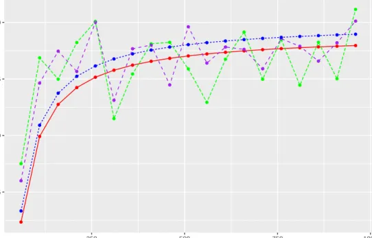
We now conduct a simulation to compare the means of the estimators and their expectations. We generate 1000 data sets from model (2.1) with µ = 10, σ2

a = 1, σ2 =

0.01, n = 1000 and m = 100. We choose r = 10 + 50k for k = 0,1, ...,19. We compute

average of ˆσ2

a,wr using formula (2.11) and its expectation using formula (2.20), and the

Jackknife estimate using formula (2.22) and its expectation using formula (2.23). Figure 2.1 shows that the average ofσˆ_a,wr2 is close to the true expected value asr increases and the Jackknife estimator has smaller bias.

● ● ● ● ● _● ● ● ● ● ● ● ● ● ● ● ● ● ● ● ● ● ● ● ● ● ● ● ● ● ● ● ● ● ● ● ● ● ● _● ● ● ● ● ● ● ● ● ● ● ● ● ● ● ● ● ● ● ● ● ● ● ● ● ● ● ● ● ● ● ● ● ● ● ● ● ● ● ● ● 0.88 0.92 0.96 1.00 0 250 500 750 1000 r Estimates of σ ^ a 2 and e xpectations

Figure 2.1: The blue line is the averages of σˆ2

a,wr, the purple line is the expectations

ofσˆ_a,wr2 , the red line is the averages of(ˆσ_a,wr∗ )2,and the green line is the expectations

of(ˆσ_a,wr∗ )2.

2.2.4

Properties of Estimators Under Sampling Without

Replace-ment of Subjects

We now consider sampling without replacement of subjects only. If we select r subjects from n subjects without replacement, then the number of selections k follows a

multi-variate hypergeometric distribution with πi = 1 n, E(ki) = r n, Var(ki) = r(n−r) n2 , and Cov(ki, kj) =− r(n−r)

n2_(n−1). The equation (2.13) becomes

ˆ µwls,wo = Pn i=1 Pm j=1 nki r2 yij mPn_i=1 nki r2 = Pn i=1 Pm j=1kiyij rm = ˆµwls,wr,

which is the same as the MLE (2.9).

Theorem 5. The conditional mean and variance of the estimator of the overall mean under sampling without replacement of subjects only are

E(ˆµwls,wo|y) = ˆµmle, (2.24) Var(ˆµwls,wo|y) = n−r rn2 n X i=1 ¯ y2_i·− 1 n−1 X i16=i2 ¯ yi1·y¯i2· ! . (2.25)

The unconditional mean, variance and MSE of the estimator of the overall mean under sampling without replacement of subjects only are

E(ˆµwls,wo) =µ, (2.26)

Var(ˆµwls,wo) =MSE(ˆµwls,wo) =

σ2 _+mσ2

a

rm , (2.27)

Proof. Since the conditional expected value of the overall mean under sampling without

replacement of subjects only is

E(ˆµwls,wo|y) = Pn i=1 Pm j=1yijE(ki) rm = Pn i=1 Pm j=1yijr_n rm = ˆµmle, then

The estimator of the overall mean under sampling without replacement is also an unbiased estimator. We have the conditional variance of µˆwls,wo

Var(ˆµwls,wo|y) =Var Pn i=1 Pm j=1kiyij rm y ! = 1 r2_m2    E n X i=1 kiyi· !2 − " E n X i=1 kiyi· !#2   = 1 r2_m2 ( _n X i1,i2=1 yi1·yi2·E(ki1ki2)− n X i1,i2=1 yi1·yi2·E(ki1)E(ki2) ) = 1 r2_m2 n X i1,i2=1 yi1·yi2·Cov(ki1ki2) = 1 r2_m2 " _n X i=1 y2_i·r(n−r) n2 − X i16=i2 yi1·yi2· r(n−r) n2_(n−1) # = n−r rn2 n X i=1 ¯ y_i2·− 1 n−1 X i16=i2 ¯ yi1·y¯i2· ! ,

then the unconditional variance of µˆwls,wo

Var(ˆµwls,wo) = E[Var(ˆµwls,wo|y)] +Var[E(ˆµwls,wo|y)]

= n−r rn2_m2 " _n X i=1 E(y_i.2)− 1 n−1 X i16=i2 E(yi1.)E(yi2.) # +Var(ˆµmle) = n−r r + 1 σ2+mσ_a2 nm = σ 2_+mσ2 a rm .

Since µˆwls,wo is an unbiased estimator, we have

MSE(ˆµwls,wo) =Var(ˆµwls,wo) =

σ2+mσ_a2

Remark 3. The estimator of the overall mean under sampling without replacement for subjects only is also an unbiased estimator. The ratio of the variances and MSEs between the subsample and the full data is n

r, which decreases to 1 as r increases to n.

The variance and MSE ofµˆwls,wo are smaller than those under sampling with replacement

by the amount of 1− 1 r σ2+mσ_a2 nm .

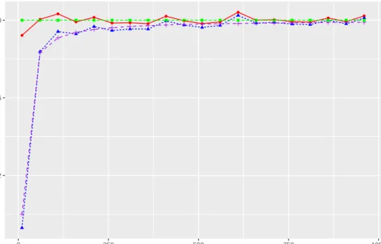
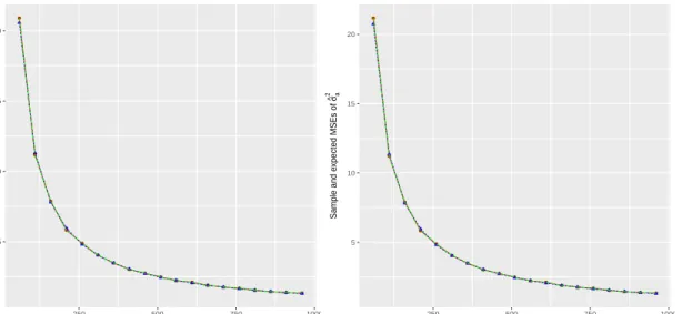
We conduct a simulation to compare the variances of the estimators and their the-oretical variances. We generate 1000 data sets from model (2.1) with µ = 10, σ2

a = 1,

σ2 _{= 0.01,n= 1000and m= 100. We chooser= 60 + 50k fork = 3, ...,18.We compute}

sample variance of µˆwls,wo, and its expected variance using formula (2.27), and sample

variance ofµˆ2

wls,wr, and its expected variance using formula (2.17). Figure 2.2 shows that

ˆ

µwls,wo has smaller variance thanµˆwls,wr.

● ● ● ● ● ● ● ● ● ● ● ● ● ● ● ● ● ● 0.0025 0.0050 0.0075 0.0100 250 500 750 1000 r Sample and e xpected v ar iances of µ ^

Figure 2.2: The green line is the sample variances of µˆwls,wr, the purple line is the

expected variances ofµˆwls,wr, the red line is the sample variances of µˆwls,wo , and the

To compare the results from the two different sampling schemes, we compute the efficiency Var(ˆµwls,wr) Var(ˆµwls,wo) = n+r−1 n = 1 + r−1 n .

Becauser is between1andn, we can see that the ratio is bigger than 1 and smaller than 2. It increases as r increases and decreases asn increases. When r n, the efficiency is close to 1.

Similar to sampling with replacement, the estimators of σ_a2 and σ2 under sampling without replacement are as follows:

ˆ

σ2_a,wo= SSAsub

rm −

RSSEsub

rm(m−1),

ˆ

σ_wo2 =RMSEsub.

Theorem 6. The conditional means of the estimators of σ2

a and σ2 under sampling

without replacement of subjects only are

E(ˆσ_a,wo2 |y) = r−1 rn + 1 n(m−1) n X i=1 ¯ y2_i·− (r−1) P i6=jy¯i·y¯j· rn(n−1) − Pn i=1 Pm j=1yij2 nm(m−1) , (2.28) E(ˆσ_wo2 |y) = Pn i=1 Pm j=1y2ij n(m−1) − mPn_i=1y¯2 i· n(m−1) . (2.29)

The unconditional means of the estimators ofσ2

a and σ2 under sampling without

replace-ment of subjects only are

E(ˆσ_a,wo2 ) = 1− 1 r σ2_a− 1 rmσ 2 , (2.30) E(ˆσ2_wo) =σ2. (2.31)

Proof. In order to get the expectation and variance of σ2

re-placement, we calculate sum of squares at first: E(SSAsub|y) =mE " _n X i=1 ki(¯yi·−y¯_..sub)2 y # =m " _n X i=1 ¯ y_i2_·E(ki)− 1 r n X i=1 ¯ y2_i·E(k_i2)−1 r X i6=j ¯ yi·y¯j·E(kikj) # =m ( r n n X i=1 ¯ y_i2_·− n X i=1 ¯ y_i2_· n−r n2 + r n2 − − n−r n2_(n−1)+ r n2 X i6=j ¯ yi·y¯j· ) = m(r−1) n n X i=1 ¯ y2_i·− 1 n−1 X i6=j ¯ yi·y¯j· ! , and E(RSSEsub|y) = E " _n X i=1 m X j=1 ki(yij −y¯i·)2 y # = n X i=1 E(ki) m X j=1 (yij −y¯i·)2 = n X i=1 r n m X j=1 y_ij2 −my¯_i2_· ! = r n n X i=1 m X j=1 y_ij2 −m n X i=1 ¯ y_i2_· ! . Then E(SSAsub) = m(r−1) n " _n X i=1 σ2+mσ2_a m +µ 2 − 1 n−1n(n−1)µ 2 # = (r−1)(σ2+mσ_a2), E(RSSEsub) = r n " _n X i=1 m X j=1 (σ2+σ_a2+µ2)−m n X i=1 σ2+mσ_a2 m +µ 2 # =r(m−1)σ2.

RSSEsub are the same as that under subsampling with replacement.

The conditional expected values of σˆ2

a,wo and σˆ2wo E(ˆσ2_a,wo|y) = E SSAsub rm − RSSEsub rm(m−1) y = r−1 rn n X i=1 ¯ y_i2_·− 1 n−1 X i6=j ¯ yi·y¯j· ! − 1 nm(m−1) n X i=1 m X j=1 y_ij2 −m n X i=1 ¯ y2_i· ! = r−1 rn + 1 n(m−1) n X i=1 ¯ y_i2_·− (r−1) rn(n−1) X i6=j ¯ yi·y¯j·− 1 nm(m−1) n X i=1 m X j=1 y_ij2, E(ˆσ_wo2 |y) = E(RSSEsub|y) r(m−1) = Pn i=1 Pm j=1y 2 ij −m Pn i=1y¯ 2 i· n(m−1) .

Taking expectation with respect to y, we have

E(ˆσ2_a,wo) = r−1 r σ2_+mσ2 a m − σ2 m = 1− 1 r σ2_a− 1 rmσ 2_, E(ˆσ2_wo) = σ2.

Remark 4. The bias ofσˆ2

a,wois larger than that based on the full data by the amount of 1 r − 1 n σ 2 a+ σ2 m

,and smaller than that ofˆσ2

a,wr by the amount of 1 n − 1 rn σ 2 a+ σ2 m . The estimator σˆ2 wo is unbiased.

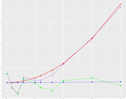
We now conduct a simulation to compare the means of the estimators and their expectations. We generate 1500 data sets from the model (2.1) with µ = 10, σ2_a = 1,

σ2 = 0.01,n = 1000and m = 100.We chooser = 10 + 50k for k = 1, ...,19. We compute

average of σˆ2

a,wo, and its expectation using formula (2.30), and average of σˆ2a,wr, and its

expectation using formula (2.20). Figure 2.3 shows thatσˆ2

● ● ● ● ● ● ● ● ● ● ● ● ● ● ● ● ● ● ● ● ● ● ● ● ● ● ● ● ● ● ● ● ● ● ● ● ● ● ● ● ● ● ● ● ● ● ● ● ● ● ● ● ● ● ● ● ● ● ● ● ● ● ● ● ● ● ● ● ● ● ● ● ● ● ● ● 0.985 0.990 0.995 1.000 250 500 750 1000 r Estimates of σ ^ a 2 and e xpectations

Figure 2.3: The green line is the average of σˆ_a,wr2 , the red line is the expectation of

ˆ

σ_a,wr2 , the purple line is the average of σˆ2_a,wo, and the blue line is the expectation of

ˆ σ_a,wo2 .

Same as the estimator σˆ2

a,wr, the estimator σˆa,wo2 is also biased with the leading term

of bias −σ

2

a

r . So we also consider the Jackknife estimator to reduce the bias

(ˆσ∗_a,wo)2 =rˆσ_a,wo,r2 −(r−1)ˆσ_a,wo,r2 ₋₁, (2.32)

where σˆ2

a,wo,r is from the sampled data with size r, and σˆa,wo,r2 −1 is the average of the leave-one-out estimators from the sampled data with size being equal tor−1. Then we have E[(ˆσ_a,wo∗ )2] =r 1− 1 r σ_a2− σ 2 rm −(r−1) 1− 1 r−1 σ2_a− σ 2 m(r−1) =σ_a2. (2.33)

of the estimators and their expectations. We generate 1000 data sets from the model (2.1) with µ= 10, σ2

a = 1, σ2 = 0.01, n = 1000 and m = 100. We choose r = 10 + 50k

fork = 0,1, ...,19.We compute average ofσˆ2

a,wo using formula (2.11), and its expectation

using formula (2.30), and average of (ˆσ∗_a,wo)2 _{using formula (2.32), and its expectation} using formula (2.33). Figure 2.4 shows that the average of σˆ2

a,wo are close to the true

expected value as r increases and the Jackknife estimator has smaller bias.

● ● ● ● ● ● ● ● ● ● ● ● ● ● ● _● ● ● ● ● 0.92 0.96 1.00 0 250 500 750 1000 r Estimates of σ ^ a 2 and e xpectations

Figure 2.4: The blue line is the average of σˆ_a,wo2 , the purple line is the expectation of

ˆ σ2

a,wo, the red line is the average of (ˆσ∗a,wo)2, and the green line is the expectation of

(ˆσ_a,wo∗ )2.

Theorem 7. The unconditional variance and MSE of the estimator ofσ_a2 under sampling without replacement of subjects only are

Var(ˆσ_a,wo2 ) =2(r−1)(σ 2 a+σ2/m)2 r2 + 2σ4 rm2_(m−1), (2.34) MSE(ˆσ_a,wo2 ) =(2r−1)(σ 2 a+σ2/m)2 r2 + 2σ4 rm2_(m−1). (2.35)

The unconditional variance and MSE of the estimator of σ2 _{under sampling without}

replacement for subjects only are

Var(ˆσ2_wo) =MSE(ˆσ_wo2 ) = 2σ

4

r(m−1). (2.36)

Proof. Given k, the residual sum of squares and sum of squares

RSSEsub= n X i=1 m X j=1 ki[yij −µ−αi−(¯yi·−µ−αi)]2 = n X i=1 m X j=1 ki(ij −¯i·)2, SSAsub=m n X i=1 ki(¯yi·−y¯sub·· )2 =m n X i=1 ki[αi+ ¯i·−( ¯α+ ¯sub·· )]2.

According to the Cochran theorem, under sampling without replacement,

n X i=1 m X j=1 ki(ij− ¯

i·)2 is independent of ¯i· and SSAsub is the function of ¯i· for i = 1, ..., n. Therefore,

RSSEsub and SSAsub are independent.

Furthermore, we have RSSEsub σ2 = Pn i=1 Pm j=1ki(ij−¯i·) 2 σ2 ∼χ 2 r(m−1), SSAsub mσ2 a+σ2 = Pn i=1ki[αi+ ¯i·−( ¯α+ ¯sub·· )]2 σ2 a+σ2/m ∼χ2_r−1.

So Var(SSAsub) =Var[mPn_i=1ki(¯yi·−y¯sub.. )2] = 2m2(r−1)(σa2+σ2/m)2and Var(RSSEsub) =

Then the variance of σˆ2

a,wo is

Var(ˆσ_a,wo2 ) =Var

SSAsub mr − RSSEsub rm(m−1) = 1

m2_r2Var(SSAsub) +

1

r2_m2_(m−1)2Var(RSSEsub)

−2Cov SSAsub mr , RSSEsub rm(m−1) =2(r−1)(σ 2 a+σ2/m)2 r2 + 2σ4 rm2_(m−1),

and the variance of σˆ2

wo

Var(ˆσ_wo2 ) = Var(RSSEsub)

r2_(m−1)2 =

2σ4

r(m−1).

Then

MSE(ˆσ_a,wo2 ) =Var(ˆσ2_a,wo) +bias2(ˆσ_a,wo2 )

=2(r−1)(σ 2 a+σ2/m)2 r2 + 2σ4 rm2_(m−1)+ 1 r2 σ_a2+σ 2 m 2 =(2r−1)(σ 2 a+σ2/m)2 r2 + 2σ4 rm2_(m−1),

and for the unbiased estimator σˆ2

wo,

MSE(ˆσ_wo2 ) =Var(ˆσ_wo2 ) = 2σ

4

r(m−1).

Remark 5. The variance ofσˆ_a,wo2 is larger than that based on full data by the amount of

1 r − 1 n 2σ4 a m2_(m−1)+2 1 r − 1 n 1− 1 r − 1 n σ 2 a+ σ2 m 2 .The MSE ofσˆ2 a,wois larger

than that based on full data by the amount of 1 r − 1 n 2− 1 r − 1 n σ 2 a+ σ2 m 2 + 1 r − 1 n 2σ4 a

m2_(m−1). The variance and MSE of σˆ 2

wo are inflated by a factor of

n

r.

We now conduct a simulation to compare the variances of the estimators and their theoretical variances. We generate 1000 data sets from the model (2.1) withµ= 10, σ2

a=

1, σ2 _{= 0.01, n = 1000 and m = 100. We choose r = 10 + 50k for k = 1, ...,19. We}

compute sample variance of σˆa,wo, and its theoretical variance using formula (2.34), and

sample variance of σˆ_a,wr2 . Figure 2.5 shows that the variance of σˆ2_a,wo is smaller that of

ˆ σ_a,wr2 . ● ● ● ● ● ● ● ● ● ● ● ● ● ● ● ● ● ● ● ● ● ● ● ● ● ● ● _● ● ● _● ● ● _● ● ● ● ● ● ● ● ● ● ● ● ● ● ● ● ● _● ● ● ● ● ● ● 0.01 0.02 0.03 250 500 750 1000 r Sample and e xpected v ar iances of σ ^ a 2

Figure 2.5: The green line is the sample variances ofσˆ2_a,wo, the red line is the

2.3

Subsampling of Both Subjects and Repeated

Mea-surements

We now consider subsampling of both subjects and repeated measurements. Suppose we want to sample r subjects from n subjects and s repeated measurements from the

m repeated measurements of those chosen subjects. We assume that rs = N. Define

Ui = ui rπs i and Cj = cj sπr j

, where ui is the number of the times that the ith subject was

chosen, cj is the number of the times that the jth repeated measurements was chosen

such that n X i=1 ui =r and m X j=1

cj =s. For simplicity, we assume that we sample repeated

measurements without replacement, so thatcj equals to one or zero. Let{πs1, ..., πns}and {πr

1, ..., πrm}be subject’s and repeated measurements’ sampling distributions, respectively.

We discuss MLE and WLS estimator for a given selected sample in Sections 2.3.1 and 2.3.2, and then discuss sampling schemes in Sections 2.3.3 and 2.3.4.

2.3.1

MLE for a Selected Subset of Both Subjects and Repeated

Measurements

We extend the MLE approach in Section 2.2.1 and McCulloch et al. [23] to this new scenario. As before we assume that observations from selected subjects are mutually independent even though some of the subjects and repeated measurements are selected more than once when sampling is done with replacement.

DefineLi(li)as the likelihood (log likelihood) of yi|(u, c), where the number of

sub-jects’ selectionsuis a vector with theith element is the number of times that the subject

i is selected and the number of repeated measurements’ selections c is a vector with the

Given c, we define yi,s to be the vector of the selected repeated measurements of

subject i. So, we have yi,s ∼ N(µ1s, Vs) with (Vs)−1 = _σ12Is− σ

2 a σ2_(σ2_+sσ2 a)Js and |V s_{| =} (σ2 _+sσ2 a)(σ2)s

−1_{. Then given u and c, L=}Qn i=1L ui i and l = Pn i=1uili, where Li =(2π)− s 2|Vs|− 1 2 exp −1 2(yi,s−µ1s) T (Vs)−1(yi,s−µ1s) , li =− s 2log(2π)− 1 2log(σ 2_+mσ2 a)− s−1 2 log(σ 2₎₋ 1 2σ2 m X j=1 cj(yij −µ)2 +σ 2 a Pm j=1cj(y rc i· −sµ)2 2σ2_(σ2_+sσ2 a) , y_irc_· = m X j=1 cjyij.

The log-likelihood function can be explicitly computed as

l =−s Pn i=1ui 2 log(2π)− 1 2log(σ 2 +sσ2_a) n X i=1 ui− s−1 2 log(σ 2 ) n X i=1 ui − 1 2σ2 n X i=1 m X j=1 uicj(yij −µ)2+ n X i=1 uicjσ2a(yirc· −sµ)2 2σ2_(σ2_+sσ2 a) . Defining SSArc_sub = n X i=1 uicj(¯yirc· −y¯··rc)2, RSSErc_sub = n X i=1 m X j=1 uicj(yij −y¯irc·)2, λ=σ2+sσ_a2, where y¯rc_i· = Pm j=1cjyij Pm j=1cj = Pm j=1cjyij s and y¯ rc ·· = Pn i=1 Pm j=1uicjyij rs = Pn i=1uiy¯rci· r . We

re-write log-likelihood function as l=− rs 2 log(2π)− r 2log(σ 2_+sσ2 a)− r(s−1) 2 log(σ 2₎₋ 1 2σ2 n X i=1 m X j=1 uicj(yij −y¯irc·)2 − 1 2σ2 n X i=1 m X j=1 uicj(¯yirc· −y¯··rc)2− 1 2σ2 n X i=1 m X j=1 uicj(¯yirc· −µ)2 + n X i=1 s2σ_a2(¯y_irc_· −µ)2 2σ2_(σ2_+sσ2 a) =− rs 2 log(2π)− r 2log(σ 2_+sσ2 a)− r(s−1) 2 log(σ 2₎₋RSSE rc sub 2σ2 − SSArc_sub 2(σ2_+sσ2 a) − rs(¯y rc · −µ)2 2(σ2_+sσ2 a) .

Then the MLEs of the overall mean and the variance components are

ˆ µrc_mle = y¯rc_.. = Pn i=1 Pm j=1uicjyij Pn i=1 Pm j=1uicj = Pn i=1 Pm j=1uicjyij N , (2.37) (ˆσ_mlerc )2 = RSSE rc sub r(s−1) =RMSE rc sub, (2.38) (ˆσrc_a,mle)2 = SSA rc sub rs − RSSErc_sub rs(s−1), (2.39)

where SSArc_sub,RSSErc_sub,MSArc_sub, and RMSErc_sub are computed from the selected subset.

2.3.2

Weighted Least Square Estimators for a Selected Subset of

Both Subject and Repeated Measurements

Again assume that observations from selected subjects are mutually independent, πs i be

the probability that the ith subject is selected, and πr_j be the probability that the jth repeated measurement is selected. A weighted least square similar to (2.12):

where V_rs = diag(Vs, ..., Vs

| {z }

r

) is the covariance matrix, D is a rs×rs diagonal rescaling

matrix with thekth diagonal element being 1/qrsπs

iπjr if the ith subject’s jth repeated

measurement in the original data was chosen for thekth trial, ST

X is ars×nm sampling

matrix with value either being zero or one, and the kth row of ST

X is e(i−1)m+j if theith

subjects’s jth repeated measurement in the original data was chosen for the kth trial. The solution to (2.40) is ˆ µrc_wls,sub = (XTW X)−1XTWy, whereW =SXDT(Vrs) −1_DST X andWi(r1, r2) = uicr2 rsπs i p πr r1π r r2 1 σ2Im− σ2 acr1 σ2_(σ2_+mσ2 a) Jm

with r1 and r2 are the position indicator numbers.

After straightforward calculation, the WLS estimator of the overall mean can be written as ˆ µrc_wls,sub = Pn i=1 Pm j=1 uicj rsπs i 1 πr jσ2 − Pm l=1 clσa2 √ πr jπrlσ2(σ2+mσa2) yij Pn i=1 Pm j=1 uicj rsπs i 1 πr jσ2 − Pm l=1 clσ2a √ πr jπrlσ2(σ2+mσ2a) . (2.41)

In practice, σ_a2 and σ2 are unknown, we plug in estimates into formula (2.41).

2.3.3

Properties of Estimators Under Sampling With

Replace-ment of Both subjects and Repeated MeasureReplace-ments

We randomly sample a subset with replacement of both subjects and repeated measure-ments and assume thatu ∼multinomial(r, πs₁, ..., π_ns)withπ_is = 1

n,c∼multinomial(s, π r 1, ..., π r m) with πr_j = 1

mean under sampling with replacement of both subjects and repeated measurements ˆ µrc_wls,wr = Pn i=1 Pm j=1 uicj rsπs i 1 πr jσ2 − Pm l=1 clσa2 √ πr jπlrσ2(σ2+mσa2) yij Pn i=1 Pm j=1 uicj rsπs i 1 πr jσ2 − Pm l=1 clσa2 √ πr jπrlσ2(σ2+mσa2) = Pn i=1 Pm j=1uicj h 1 σ2 − sσ2 a σ2_(σ2_+mσ2 a) i yij Pn i=1 Pm j=1uicj h 1 σ2 − sσ2 a σ2_(σ2_+mσ2 a) i = Pn i=1 Pm j=1uicjyij N .

We note that the estimator of the overall mean is the same as the MLE in (2.37).

Theorem 8. The conditional mean and variance of the estimator of the overall mean under sampling with replacement of both subjects and repeated measurements are

E(ˆµrc_wls,wr|y) =ˆµmle, (2.42) Var(ˆµrc_wls,wr|y) = 1 N2 rs(m−1)(r+n−1) n2_m2 n X i=1 m X j=1 y2_ij −rs(r+n−1) n2_m2 n X i=1 X j16=j2 yij1yij2 + rs 2_(n−1) n2 n X i=1 (¯y_irc_·)2+ rs(r−1)(s+m−1) n2_m2 X i16=i2 m X j=1 yi1jyi2j + rs(r−1)(s−1) n2_m2 X i16=i2 X j16=j2 yi1j1yi2j2 − r2_s2 n2 X i16=i2 ¯ yrc_i 1·y¯ rc i2· . (2.43)

The unconditional mean and variance of the estimator of the overall mean under sampling with replacement of both subjects and repeated measurements are

E(ˆµrc_wls,wr) =µ, (2.44) Var(ˆµrc_wls,wr) =MSE(ˆµrc_wls,wr) = 1 r + 1 n − 1 rn σ 2 a+ (s+m−1)σ2 sm . (2.45)

both subjects and repeated measurements is E(ˆµrc_wls,wr|y) =E Pn i=1 Pm j=1uicjyij N y ! = Pn i=1 Pm j=1E(ui)E(cj)yij N = Pn i=1 Pm j=1yij nm ,

then the unconditional expectation of the estimator of the overall mean

E(ˆµrc_wls,wr) =E[E(ˆµrc_wls,wr|y)] =E Pn i=1 Pm j=1yij nm ! = Pn i=1 Pm j=1E(µ+αi+ij) nm =µ.

According to the distributions of ui and cj, we know that E(ui) = rπis =

r n, Var(ui) = rπ_is(1−π_is) = r n 1− 1 n , Cov(ui1, ui2) =−rπ s i1π s i2 =− r n2,E(cj) = sπ r j = s m, Var(cj) = sπ_jr(1−π_jr) = s m 1− 1 m , and Cov(cj1, cj2) = −sπ r j1π r j2 =− s m2.

In order to get the conditional and unconditional variances of the estimator of the overall mean under sampling with replacement of both subjects and repeated measure-ments, we derive the following results first:

E m X j=1 cjyij y ! = m X j=1 E(cj)yij = s m m X j=1 yij, then E m X j=1 cjyij ! =sµ. Since Var m X j=1 cjyij y ! = m X j=1 y_ij2Var(cj) + X j16=j2 yij1yij2Cov(cj1, cj2) =s(m−1) m2 m X j=1 y2_ij − s m2 X j16=j2 yij1yij2,

then the unconditional variance Var m X j=1 cjyij ! =E " Var m X j=1 cjyij y !# +Var " E m X j=1 cjyij y !# = s(m−1) m2 m X j=1 [Var(yij) +E2(yij)]− sP j16=j2(σ 2 a+µ2) m2 +Var s m m X j=1 yij ! = s(m−1) m2 m X j=1 (σ_a2+σ2+µ2)− s(m−1)(σ 2 a+µ2) m +s 2 σ2_a+ σ 2 m =s2σ_a2+s(s+m−1)σ 2 m. Letai =Pm_j=1cjyij,we have E(ai1ai2|y) =E m X j=1 cjyi1j m X j=1 cjyi2j y ! =E m X j=1 c2_jyi1jyi2j y ! +E X j16=j2 cj1cj2yi1j1yi2j2 y ! = m X j=1 yi1jyi2j[Var(cj) +E 2_(c j)] + X j16=j2 yi1j1yi2j2E(cj1cj2) =s 2_+sm−s m2 m X j=1 yi1jyi2j+ s2−s m2 X j16=j2 yi1j1yi2j2.

mean under sampling with replacement of both subjects and repeated measurements Var(ˆµrc_wls,wr|y) =Var( Pn i=1 Pm j=1uicjyij|y) N2 = Var(Pn_i=1uiai|y) N2 = 1 N2    E n X i=1 uiai y !2 − " E n X i=1 uiai y !#2   = 1 N2    n X i=1 E(u2_ia2_i|y) + X i16=i2 E(ui1ui2ai1ai2)− n X i=1 r ns¯y rc i· !2   = 1 N2 n X i=1 E(u2_i) " s(m−1) m2 m X j=1 y2_ij− s m2 X j16=j2 yij1yij2 +s 2_(¯yrc i·)2 # + X i16=i2 E(ui1ui2) " s2_+sm−s m2 m X j=1 yi1jyi2j+ s2_−s m2 X j16=j2 yi1j1yi2j2 # − r 2_s2 n2 " _n X i=1 (¯yrc_i·)2+ X i16=i2 ¯ yrc_i1·y¯irc2· # = 1 N2 rs(m−1)(r+n−1) n2_m2 n X i=1 m X j=1 y2_ij −rs(r+n−1) n2_m2 n X i=1 X j16=j2 yij1yij2 + rs 2_(n−1) n2 n X i=1 (¯y_irc_·)2+ rs(r−1)(s+m−1) n2_m2 X i16=i2 m X j=1 yi1jyi2j + rs(r−1)(s−1) n2_m2 X i16=i2 X j16=j2 yi1j1yi2j2 − r2_s2 n2 X i16=i2 ¯ yrc_i 1·y¯ rc i2· ,

replacement of both subjects and repeated measurements

Var(ˆµrc_wls,wr) =E[Var(ˆµrc_wr,sub|y)] +Var[E(ˆµrc_wr,sub|y)]

= 1 N2 rs(m−1)(r+n−1) n2_m2 n X i=1 m X j=1 E(y_ij2)− rs(r+n−1) n2_m2 n X i=1 X j16=j2 E(yij1yij2) + rs 2_(n−1) n2 n X i=1 E(¯y_irc_·)2+ rs(r−1)(s+m−1) n2_m2 X i16=i2 m X j=1 E(yi1jyi2j) + rs(r−1)(s−1) n2_m2 X i16=i2 X j16=j2 E(yi1j1yi2j2)− r2_s2 n2 X i16=i2 E(¯yrc_i 1·y¯ rc i2·) +Var Pn i=1 Pm j=1yij nm ! =1 N (m−1)(r+n−1) nm (σ 2 a+σ2+µ2)− r+n−1 nm (m−1)(σ 2 a+µ2) + s(n−1) n σ2_a+ σ 2 m +Var( Pn i=1y¯ rc i·) n2 =1 N (m−1)(r+n−1) nm σ 2₊s(n−1) n σ2_a+ σ 2 m +σ 2 a+σ2/m n = 1 r + 1 n − 1 rn σ 2 a+ (s+m−1)σ2 sm .

Since µˆrc_wls,wr is unbiased, then

MSE(ˆµrc_wls,wr) =Var(ˆµrc_wls,wr) = 1 r + 1 n − 1 rn σ 2 a+ (s+m−1)σ2 sm .

Remark 6. The estimator of the overall mean under sampling with replacement of both subjects and repeated measurements µˆrc_wls,wr =

Pn i=1

Pm

j=1uicjyij

N is an unbiased

estimator. The variance and MSE of µˆrc

wls,wr are larger than those based on the full data

by the amount of 1 r 1− 1 n (n−1)σ2 a rn + m−1 s + n−1 r + (n−1)(m−1) rs σ2 nm. With

the fixedN, the MSE ofµˆrc_wls,wrachieves the minimum when r=

s

N(n−1)(mσ2

a+σ2)

(m−1)σ2 .

Theorem 9. The conditional means of the estimators of σ2

a and σ2 under sampling with

replacement of both subjects and repeated measurements are

E[(ˆσ_a,wrrc )2|y] =(r−1)(n−1)(m+s−1)−rn(m−1) rsn2_m2 n X i=1 m X j=1 y_ij2 + (r−1)(n−1)(s−1) +rn rsn2_m2 n X i=1 X j16=j2 yij1yij2 − r−1 rsn2_m2 " (s+m−1)X i16=i2 m X j=1 yi1jyi2j + (s−1) X i16=i2 X j16=j2 yi1j1yi2j2 # , (2.46) E[(ˆσ_wrrc)2|y] =m−1 nm2 n X i=1 m X j=1 y_ij2 − 1 nm2 n X i=1 X j16=j2 yij1yij2. (2.47)

The unconditional means of the estimators ofσ_a2 andσ2 under sampling with replacement of both subjects and repeated measurements are

E[(ˆσ_a,wrrc )2] = 1− 1 r 1− 1 n σ2_a+ r N n 1 m −1 + 1 rm 1 n −1 σ2 + 1 m − N + 1 nm + 1 N 1 n + 1 m −1 σ2, (2.48) E[(ˆσ_wrrc)2] = 1− 1 m σ2. (2.49) Proof. Because of E(¯yrc_i·) = E Pm j=1cjyij s ! = su s = u, Var(¯y rc i·) = Var(Pm_j=1cjyij) s2 = σ_a2+ (s+m−1)σ 2

sm, and the independence among subjects, we have

¯ y_irc_· iid∼ N µ, σ_a2+ 1 m + 1 s − 1 sm σ2 .

As we also assumed,ui’s,cj’s andy’s are mutually independent, so the expectations and

variances of the conditional and unconditional sum of squares can be derived as follows

E(SSArc_wr,sub|y) =sE " _n X i=1 ui(¯yirc· −y¯rc.. )2 y # =s n X i=1 E[(¯y_irc_·)2|y]E(ui)− 1 r n X i=1 E[(¯y_irc_·)2|y]E(u2_i) − 1 r X i16=i2 E(¯yrc_i1.y¯_irc_2.|y)E(ui1ui2) =s rn−r−n+ 1 n2 n X i=1 m+s−1 sm2 m X j=1 y2_ij +s−1 sm2 X j16=j2 yij1yij2 ! − r−1 n2 X i16=i2 s+m−1 sm2 m X j=1 yi1jyi2j + s−1 sm2 X j16=j2 yi1j1yi2j2 ! =rn−r−n+ 1 n2_m2 " (m+s−1) n X i=1 m X j=1 y_ij2 + (s−1) n X i=1 X j16=j2 yij1yij2 # − r−1 n2_m2 " (s+m−1)X i16=i2 m X j=1 yi1jyi2j + (s−1) X i16=i2 X j16=j2 yi1j1yi2j2 # , and E(RSSErc_wr,sub|y) =E " _n X i=1 m X j=1 uicj(yij −y¯irc·)2 y # = n X i=1 m X j=1 E(ui)E(cj)y2ij − 1 s n X i=1 E(ui)E   m X j=1 cjyij !2 y   =r(s−1)(m−1) nm2 n X i=1 m X j=1 y2_ij −r(s−1) nm2 n X i=1 X j16=j2 yij1yij2.

Then E(SSArc_wr,sub) =(r−1)(n−1)(m+s−1) n2_m2 n X i=1 m X j=1 (σ2+σ_a2+µ2) + (r−1)(n−1)(s−1) n2_m2 n X i=1 X j16=j2 (σ_a2+µ2) − r−1 n2_m2[(m+s−1) X i16=i2 m X j=1 µ2+ (s−1)X i16=i2 X j16=j2 µ2] =(r−1)(n−1) n sσ_a2+m+s−1 m σ 2 , and E(RSSErc_wr,sub) =r(s−1)(m−1) nm2 n X i=1 m X j=1 (σ2+σ_a2+µ2)− r(s−1) nm2 n X i=1 X j16=j2 (σ2_a+µ2) =r(s−1)(m−1) m σ 2_.

Consequently, we get the conditional expected value of (ˆσrc a,wr)2 E[(ˆσ_a,wrrc )2|y] =E _SSArc wr,sub rs − RSSErc_wr,sub rs(s−1) y =(r−1)(n−1)(m+s−1)−rn(m−1) rsn2_m2 n X i=1 m X j=1 y_ij2 + (r−1)(n−1)(s−1) +rn rsn2_m2 n X i=1 X j16=j2 yij1yij2 − r−1 rsn2_m2 (s+m−1)X i16=i2 m X j=1 yi1jyi2j + (s−1) X i16=i2 X j16=j2 yi1j1yi2j2 ,

and the conditional mean of (ˆσrc_wr)2

E[(ˆσ_wrrc)2|y] = E(RSSE rc wr,sub|y) r(s−1) = m−1 nm2 n X i=1 m X j=1 y_ij2 − 1 nm2 n X i=1 X j16=j2 yij1yij2.

Taking expectation with respect to y, we have E[(ˆσ_a,wrrc )2] =E _SSArc wr,sub rs − RSSErc_wr,sub rs(s−1) =(r−1)(n−1) rn σ 2 a+ (r−1)(n−1)(m+s−1) rn −m+ 1 σ2 sm = 1− 1 r 1− 1 n σ2_a+ r N n 1 m −1 + 1 rm 1 n −1 σ2 + 1 m − N + 1 nm + 1 N 1 n + 1 m −1 σ2, and E[(ˆσ_wrrc)2] =EE[(ˆσrc_wr)2|y] = 1− 1 m σ2.

Remark 7. The bias of (ˆσrc

a,wr)2 is larger than that of the full data by the amount of

1 r 1− 1 n σ_a2− 1− 1 r 1− 1 n m−1 s + 1 − m−1 s + 1 n σ2 m.

As we can see from the formula, the major term of the unconditional expected values of

(ˆσrc

a,wr)2 increases as r increases. The expectation of(ˆσwrrc)2 is smaller than that based on

the full data by the amount of σ 2

a

m. The calculation of the variances of(ˆσ

rc

a,wr)2 and(ˆσrcwr)2

are too complicated, we will use simulations to investigate them later.

2.3.4

Properties of Estimators Under Sampling Without

Replace-ment of Both Subjects and Repeated MeasureReplace-ments

We now consider sampling without replacement of both subjects and repeated measure-men