An iterative Newton\u27s method for output-feedback LQR design for large-scale systems with guaranteed convergence

large-scale systems with guaranteed convergence

Downloaded from: https://research.chalmers.se, 2020-01-17 16:05 UTC

Citation for the original published paper (version of record):

Ilka, A., Murgovski, N., Sjöberg, J. (2019)

An iterative Newton's method for output-feedback LQR design for large-scale systems with

guaranteed convergence

2019 18th European Control Conference (ECC), June 2019: 4849-4854

http://dx.doi.org/10.23919/ECC.2019.8795752

N.B. When citing this work, cite the original published paper.

research.chalmers.se offers the possibility of retrieving research publications produced at Chalmers University of Technology. It covers all kind of research output: articles, dissertations, conference papers, reports etc. since 2004.

research.chalmers.se is administrated and maintained by Chalmers Library

An iterative Newton’s method for output-feedback LQR design

for large-scale systems with guaranteed convergence*

Adrian Ilka

, Nikolce Murgovski

and Jonas Sj¨oberg

Abstract— The paper proposes a novel iterative output-feedback control design procedure, with necessary and suf-ficient stability conditions, for linear time-invariant systems within the linear quadratic regulator (LQR) framework. The proposed iterative method has a guaranteed convergence from an initial Lyapunov matrix, obtained for any stabilizing state-feedback gain, to a stabilizing output-state-feedback solution. An-other contribution of the proposed method is that it is compu-tationally much more tractable then algorithms in the literature, since it solves only a Lyapunov equation at each iteration step. Therefore, the proposed algorithm succeed in high dimensional problems where other, state-of-the-art methods fails. Finally, numerical examples illustrate the effectiveness of the proposed method.

I. INTRODUCTION

One of the most fundamental problems in control theory is the linear quadratic regulator (LQR) design problem [1]. The so-called infinite horizon linear quadratic problem of finding a control functionu∗(t) =Kx(t)for x0∈Rnx _that minimizes the cost functional:

J∗= Z ∞ 0 x(t)TQx(t) +uT(t)Ru(t) + 2xT(t)N u(t)dt, (1)

withR >0,Q−N R−1NT ≥0 subject tox(0) =x0, and

˙

x(t) =Ax(t) +Bu(t),

y(t) =Cx(t) +Du(t), (2) has been studied by many authors [1], [2], [3], [4]. In the equations above x(t) ∈ Rnx_{, y(t) ∈}

Rny_{, and u(t) ∈} Rnu _{denote the state, measurable output, and the} con-trol input vectors, respectively. Furthermore, matrices A ∈

Rnx×nx_{, B} ∈

Rnx×nu_{, C} ∈

Rny×nx_{, and D} ∈

Rny×nu are constant known matrices. Given a symmetric matrix P =PT _∈

Rn×n, the inequality P > 0 (P ≥ 0) denotes

that P is positive (semi) definite. Matrices, if not explicitly stated, are assumed to have compatible dimensions.

Often it is not possible or economically feasible to measure all the state variables. In this case, an output-feedback control law defined as

u(t) =F y(t), (3) would be more beneficial. However, finding an optimal output-feedback control law in the form (3), which mini-mizes (1), is still one of the most important open questions

*This work has been financed in part by the Swedish Energy Agency (P43322-1), and by IMPERIUM (H2020 GV-06-2015).

1_{Department of Electrical Engineering, Chalmers University of}

Technology, H¨orsalsv¨agen 9-11, SE-412 96, Gothenburg, Sweden.

[email protected]

in control engineering, despite the availability of many approaches and numerical algorithms, as it is pointed out in survey papers [5], [6]. This is mainly due to the lack of testable necessary and sufficient conditions for output-feedback stabilizability, and/or the limitations of the available approaches.

Non-testable sufficient conditions for output-feedback sta-bilizability within the LQR framework are mostly formulated as coupled nonlinear equalities or linear/bilinear matrix in-equalities (LMIs/BMIs) [7], [8], [9], [10]. The majority of algorithms for output-feedback LQR design are formulated in terms of LMIs [11], [12], [13], [14], [15], [16], [17] or BMIs [18], [10], [19], [20], [21], [22]. These algorithms are dependent on the used LMI or BMI solvers and could work well for small-sized problems, but may fail as the problem size increases (due to solver limitations). In addition, avail-able iterative numerical algorithms with convergence such as [23], [24], or algorithms using nonlinear programming such as [25], [26], unfortunately require a selection of an initial stabilizing output-feedback gain. However, a direct procedure for finding such a gain is unknown and could be hard to get, as discussed in [5]. Finally, authors in [8] proposed a promising iterative algorithm which iterates a Riccati equation from an initial state-feedback solution, however the convergence has not been proven.

Inspired by [8], in this paper we propose an alterna-tive way for output-feedback LQR design for linear time-invariant (LTI) systems, using a modified Newton’s method with guaranteed convergence to an output-feedback solution from any stabilizing state-feedback gain, more precisely, from a Lyapunov matrix for any stabilizing state-feedback gain. Furthermore, the proposed algorithm requires solving only a Lyapunov equation at each iteration step, which is computationally much more tractable then algorithms in the literature, including approaches based on LMIs and/or BMIs. II. NECESSARY AND SUFFICIENT CONDITIONS

FOR OUTPUT-FEEDBACK STABILIZABILITY This section formulates the necessary and sufficient stabil-ity conditions for output-feedback stabilizabilstabil-ity in the LQR framework, adopted and modified from [8]. In the rest of the paper it is assumed without loss of generality that in the system (2) the matrixD is zero, see for example [27].

Considering the system (2) and the output-feedback con-trol low (3), let us recall some related terminology.

Definition 1. A square matrix A ∈ Rnx×nx _{is said to} be stable if and only if for every eigenvalues λi of A,

Definition 2. The pair (A, B) is said to be stabilizable if and only if there exist a real matrixK∈Rnu×nx _{such that} A−BK is stable.

Definition 3. The pair (A, C) is said to be detectable if and only if there exist a real matrix L∈_Rnx×ny _{such that} A−LC is stable.

Definition 4. The system (2) is said to be static output-feedback stabilizableif and only if there exist a real matrix F ∈Rnu×ny _{such that A−BF C is stable.}

Theorem 1. The following statements are equivalent. 1) The system (2)is static output-feedback stabilizable. 2) The pair (A, B) is stabilizable, the pair (A, C) is

detectable and there exist real matrices F ∈ Rnu×ny and G∈Rnu×nx _{such that}

F C−R−1(BTP+NT) =G, (4) where P ∈ Rnx×nx _{is the real symmetric} positive-definite solution of R(P) =ATP+P A+Q+GTRG −(P B+N)R−1(BTP+NT) = 0, (5) for givenQ∈Rnx×nx_{,N ∈} Rnx×nu _andR∈ Rnu×nu matrices satisfying Q, N NT_{, R} ≥0, R≥0. (6) Proof. Assume that the first condition holds that isA−BF C is stable, for some F. Then the pair (A, B) is stabilizable since A−BK is stable for K = F C, and consequently the pair (A, C) is detectable, since A−LC is stable for L =BF. Furthermore, becauseA−BF C is stable, there exists a unique symmetric positive-definite matrixP(see [8], [28] for details), such that

R(P) = (A−BF C)TP+P(A−BF C) +Q

+CTFTRF C−CTFTNT−N F C= 0. (7) Rearranging (7), one can obtain

R(P) =ATP+P A+Q −(P B+N)R−1(BTP+NT) +F C−R−1(BTP+NT) T RF C −R−1(BTP+NT)= 0. (8)

Hence, setting G = F C−R−1(BTP +NT) implies that equation (4) exists.

Now assume that the second condition holds. From equa-tion (4) follows that (7) is satisfied. From the second con-dition follows that A−LC is stable for some L. Noting that (A−LC) = (A−BF C)−[L, −B] C F C , (9)

it follows that the pair

A−BF C, C F C is detectable as well. Since P is symmetric and positive-definite, we conclude from (7) thatA−BF C is stable, [8], [28].

The next corollary is straightforward. Corollary 1. Suppose that

K=R−1(BTP+NT),

F =KCT(CCT)−1, andG=F C−K, then the following statements are equivalent,

1) R(P) =ATP+P A+Q+GTRG −(P B+N)R−1(BTP+NT), (10) 2) R(P) = ˜Q+GTRG+ ˜ATP+PA˜−PSP,˜ (11) where ˜ A=A−BR−1NT, S˜=BR−1BT, ˜ Q=Q−N R−1NT.

Proof. The equivalence can be proved by substituting back all the denotations.

III. MODIFIED NEWTON’S METHOD FOR INFI-NITE HORIZON OUTPUT-FEEDBACK LQR DESIGN

The equations (10) and (11) are algebraic Riccati-like equations. In general, Newton’s method and it’s modifica-tions are widely used to solve algebraic Riccati equamodifica-tions [29], [30], [31], [32]. Inspired by [29] and [30] we propose a modified Newton’s method to solve the infinite horizon output-feedback LQR problem, i.e. to find a control law in the form (3) for the system (2), minimizing the cost function defined as (1).

ConsiderS as a Banach space for any matrix norm, then

Ris mapping fromS into itself. The first Fr´echet derivative of (11) at the matrix P is a linear mapR0_P˜ :S → S given

by R0P(X) =H T 1(P)X+XH1(P) +H2T(P)XZ +ZTXH2(P), (12) whereZ=CT_(CCT₎−1_{C, and} H1(P) = ˜A−SP Z˜ −BR−1NTZ+BR−1NT, H2(P) = ˜SP−SP Z˜ +BR−1NT −BR−1NTZ.

Then the Newton’s method for the solution of (11) for the j-th iteration is

Pj+1=Pj+ (R0Pj)

−1_R(P

j), j= 1,2, . . . . (13) Considering (12) and (13), we can write

H₁T(Pj)Xj+XjH1(Pj) +H2T(Pj)XjZ +ZTXjH2(Pj) =−R(Pj),

(14) Pj+1=Pj+Xj, j= 1,2, . . . . (15)

The equation (14) is a coupled Sylvester equation, which can be solved by gradient-based iterative methods such as [33], [34] and [35]. However, by freezing the matrix G in (11), the termGT_{RGbecomes a constant during an iteration step} and the Fr´echet derivative reduces to

ˆ

R0P(X) = ( ˜A−SP˜ )TX+X( ˜A−SP˜ ), (16) and the Newton’s method for the j-th iteration to

( ˜A−SP˜ j)TXj+Xj( ˜A−SP˜ j) =−R(Pj), (17) Pj+1=Pj+Xj, j= 1,2, . . . , (18) where

R(Pj) = ˜Q+GTjRGj+ ˜ATPj+PjA˜−PjSP˜ j. (19) The equation (17) is a Lyapunov equation, which can be solved efficiently and with much less computational effort (and computational time) then solving (14) with iterative methods. By this modification we loose the quadratic conver-gence, but we can still prove that under certain assumptions it converges (at least linearly) to a solution.

The next Algorithm summarizes the proposed modified Newton’s method for infinite-horizon output-feedback LQR design using (16)–(19).

Algorithm 1: Modified Newton’s method for output-feedback LQR design

1 Choose some stabilizing initial guessP0=P0T;

2 forj=1:max iterationdo

3 Fj=R−1(BTPj+NT)CT(CCT)−1 ; 4 Gj=FjC−R−1(BTPj+NT); 5 R(Pj) = ˜Q+GTjRGj+ ˜ATPj+PjA˜−PjSP˜ j; 6 iftrace(R(Pj)TR(Pj))> then 7 Xj ←( ˜A−SP˜ j)TXj+Xj( ˜A−SP˜ j) =−R(Pj); 8 Pj+1=Pj+Xj; 9 else 10 break; 11 end 12 end A. Convergence

In this subsection, we show that under certain assumptions, Algorithm 1 has a guaranteed convergence from a stabilizing starting guessP0 (i.e. A˜−SP˜ 0 is stable for someQ˜ ≥0),

to a stabilizing output-feedback solution.

Remark 1. If system (2) is stabilizable and detectable, then the standard state-feedback LQR solution for (2) for some

˜

Q≥0always gives a P0for which A˜−SP˜ 0 is stable.

Let us recall some results relating to the convergence proof.

Definition 5. Theinertiaof a matrixW ∈_Rn×n_{is the triple} In(W) = (π(W), ν(W), δ(W)) where π(W), ν(W), and δ(W)are the number of eigenvalues with positive, negative, and zero real part respectively.

Lemma 1. IfH =HT ∈Rn×n,A∈Rn×n, and W >0∈ Rn×n satisfyAH+HAT =−W ≤0, andδ(A) = 0, then In(−H)≤In(A).

Proof. For proof see [36, Proposition 1, p. 447]. Lemma 2. Let H = HT _∈

Rn×n,A ∈ Rn×n, W >0 ∈ Rn×n and C ∈Rl×n satisfy AH+HAT =−W ≤CTC, where (A, C) defines a detectable pair. Then ν(A) =n if and only ifν(H) = 0, [29, Lemma 8, p. 5] .

Proof. If Ais stable, soν(A) =n, thenν(H) = 0 follows from Lemma 1. Ifν(H) = 0, soH is positive semidefinite, thenν(A) =n. To prove that we assume the contrapositive, i.e.,Ahas at least one eigenvalue λwithRe(λ)≥0. Since the pair(A, C)is detectable, Cw6= 0, wherewdenotes the corresponding right eigenvector. Thus, we obtain:

wH(AH+HAT)w= 2Re(λ)wHHw

≤ −wHCTCw <0, (20) which contradicts the positive semidefiniteness of H.

The next Proposition shows that if the conditions described in Theorem 1 hold, then with a stabilizing starting guess (P0) the Algorithm 1 cannot fail due to a singular Lyapunov

operator.

Proposition 1. Suppose that the conditions in Theorem 1 hold, so the pair ( ˜A,C˜q) is detectable, where Q˜ = ˜CqTC˜q is a full-rank factorisation of Q˜. If X0 is stabilizing, and Algorithm 1 is applied to(11), then the Lyapunov operator ˜

Ωj in step 7 from Algorithm 1 is nonsingular for all j and the sequence of approximate solutionsXj is well defined. Proof. Suppose that the pair( ˜A,C˜q)is detectable. From step 7 from Algorithm 1 applied to (11) we can get

( ˜A−SP˜ j)T(Pj+Xj) + ( ˜A−SP˜ j)(Pj+Xj) =−Q˜−GTjRGj−PjSP˜ j ≤ −Q,˜

(21) sinceQ˜ andS˜ are positive semidefinite, due to the positive semidefiniteness ofQ−N R−1_NT _{andR. From (21) follows} that ifA˜−SP˜ j is stable, thenA˜−S˜(Pj+Xj)is also stable. Furthermore, Lemma 2 implies that Pj +Xj is positive semidefintie. The Lyapunov operator corresponding to the Lyapunov equation in step 7 from Algorithm 1 is well defined, precisely as:

˜

Ωj(Xj) = ( ˜A−SP˜ j)TXj+Xj( ˜A−SP˜ j), (22) forXj∈Rnx×nx _{andj = 1,2, . . ..}

Let us recall the following Lemma.

Lemma 3. Suppose that{Pj}∞j=1is a sequence of symmetric matrices such that {R(Pj)}∞j=1 is bounded. If the pair

( ˜A, B)is stabilizable andA˜−SP˜ j is stable for eachj≥0, then{Pj}∞j=1 is bounded.

Proof. For proof see [30, Lemma 2.3].

Collecting the results so far, we have the following con-vergence result for the modified Newton’s method.

Theorem 2. Suppose that the pair( ˜A, B)is stabilizable, the pair ( ˜A,C˜q) is detectable, and there exist real matrices F andGsuch thatF C−R−1(BTP+NT) =G. If Algorithm 1 is applied to(11)with a stabilizing starting guessP0(i.e.A˜− BK0is stable for someQ˜ ≥0), thenP∗= limj→∞Pjexists and is the stabilizing solution of the generalized Riccati-like equation (11).

Proof. The proof follows from Theorem 1, Lemmas 1, 2, 3 and Proposition 1.

Remark 2. From Theorem 2 follows that the convergence rate of Algorithm 1 is at least sublinear. In the examples we studied that the convergence rate is in fact linear, although further investigation is needed to show if the convergence rate is strictly linear.

Remark 3. Control law (3) is defined in a static output-feedback (SOF) form. Many controller structures can be transformed to this SOF form (like proportional-integral PI, proportional-integral-derivative PID, proportional-derivative PD, even full/reduced order dynamic output-feedback con-trollers) by augmenting the system with additional state variables. For more info, see [17].

IV. NUMERICAL EXAMPLES

In order to show the viability of the previous proposed method, the COMPleib [37] library has been used. For better highlighting the benefits of the proposed method, the iterative LMI (iLMI) method from [17] and the BMI formulation of the ofLQR problem (Lemma 4) have been evaluated on the COMPleib library as well.

Lemma 4. The static output-feedback LQR design problem is equivalent with the following optimization problem

min F,P(x T 0P x0) (23) subject to ( ˜A−BF C)TP+P( ˜A−BF C) + ˜Q+CTFTRF C≤0, (24) P >0, (25)

Proof. Assume that the Lyapunov candidate

V(x(t)) =x(t)TP x(t), (26) is positive definite. Then from the Bellman-Lyapunov in-equality follows

˙

V(x(t)) +J(x(t))≤0→V˙(x(t))≤ −J(x(t)), (27) where

J =x(t)TQx˜ (t)≥0, (28) which indicates that the closed-loop system is stable. Inte-grating both sides from 0 to ∞ we can obtain the upper bound of the cost function

J∞≤V(x(0))−V(x(∞))≤x(0)TP x(0), (29)

which completes the proof.

All numerical solutions, have been carried out on HP EliteBook 820 (Intel CORE i7-5600u 2.60 GHz CPU, 16 GB RAM) laptop computer using Matlab 2017a [38]. Fur-thermore, BMI and iLMI formulations have been carried out by Penlab BMI solver [39] and by Mosek LMI solver [40] using YALMIP R20150918 [41]. Finally, for the proposed method (Algorithm 1) for the step 7 the built-in Matlablyap subrutin has been used.

Numerical results for all static output-feedback stabilizable plants in COMPleib for Q = CTC, R = I, N = 0, and x0i = 1, i = 1, . . . , nx, are shown in Table I. The results indicates that the proposed approach is superior compared to BMI and iLMI formulations. In addition, even with the built-in Matlablyapsubrutin, which is not well-suited for large-scale problems, we where able to solve examples with order higher then 4000 within minutes. The LAH example well demonstrates that the proposed approach is computationally much more tractable then approaches based on LMIs and/or BMIs. While the Algorithm 1 converged to a solution in2.84 milliseconds, it took 38 seconds for the iLMI formulation, and8.31hours for the BMI one.

Table I also indicates that most of the examples in the COMPleib library are ill-posed and therefore the residual is also ill-conditioned. Due to this, in many cases the Q=CT_{Chas negative eigenvalues, while Q≥0 is needed} for the convergence. Furthermore, it can be stated that if the condition number (using Frobenius norm) of the residual (11) is higher than 1×1016 _{then the proposed algorithm}

often fails to converge to a solution. The only one exception is the plant NN17, however the condition number is still big (3.71×1015_{) which could cause numerical problems.}

From this follows that system scaling or using some pre-conditioning techniques is recommended for ill-posed and/or ill-conditioned problems. The same applies for the iLMI and BMI formulations.

Beside these, the proposed algorithm was still able to find a solution for plenty of examples without any scaling and/or preconditioning, even with negative eigenvalues in Q=CT_{C in Matlab, and for condition number of the} residual (11)R(P0)higher than1×1016. Let us note that for

examples where the condition number for R(P0) was less

then1×1010 _{the Algorithm 1 converged within 2-3 steps.}

In Table I superscripts indicate that

1 _{for the given plantQ=C}T_{Chas negative eigenvalues in} Matlab,

2 _{for the given plant the condition number of the residual}

R(P0)is higher than 1×1016, where P0 is the solution

of the state-feedback LQR design,

3 _{for the given plant the pair (A}˜_{,B) is not stabilizable.} Remark 4. The first and third condition is prerequisite even for the standard LQR design (i.e. for state-feedback LQR design).

Remark 5. The differences in the values ofxT

0P x0between

the iLMI/BMI formulations and the proposed method (Al-gorithm 1) are due to the differences in the problem formu-lation. In general the output-feedback LQR problem is not

TABLE I

OUTPUT-FEEDBACKLQRBENCHMARKS ONCOMPleIB PLANTS

Problem description BMI formulation (Lemma 4) iLMI formulation (oflqr toolbox [17]) Proposed method (Algorithm 1)

(Penlab BMI solver) (Mosek LMI solver) (Matlab lyap subrutin) Name nx ny nu cond(R(P0))F Iter. Time(s) x0TP x0 Iter. Time(s) xT0P x0 Iter. Time(s) xT0P x0 AC1 5 3 3 1.41E+15 - - - 103 2.02E-02 1.74E+01

AC2 5 3 3 1.41E+15 - - - 103 1.57E-02 1.74E+01

AC3 5 4 2 7.99E+15 - - - 32 1.92E+01 2.49E+01 19 3.40E-03 1.97E+01

AC42 _{4 2 1 Inf - - - 4 2.42E+00 4.66E-01 15 2.19E-03 4.71E-01} AC5 4 2 2 3.58E+10 - - - 13 3.22E-03 1.58E+06

AC61 _{7 4 2 4.82E+15 - - - 62 3.72E+01 1.08E+01 112 2.49E-02 1.23E+01} AC71,2 _{9 2 1 2.15E+16 - - - 15 9.07E+00 7.76E-01 24 7.25E-03 7.66E-01} AC81,2 _{9 5 1 4.66E+17 - - - 5 3.06E+00 3.73E+01 9 1.92E-02 1.09E+01} AC91,2 _{10 5 4 1.02E+19 - - - - - - - -} -AC101,2 _{55 2 2 9.04E+19 - - - - - - - -} -AC11 5 4 2 9.48E+13 - - - 389 6.11E-02 1.15E+02

AC12 4 4 3 1.37E+06 - - - 2 1.50E+00 1.05E+04 1 1.41E-04 1.05E+04

AC131,2 _{28 4 3 5.30E+20 - - - - - - - -}

-AC141,2 _{40 4 3 Inf - - - - - - - -}

-AC15 4 3 2 9.70E+15 - - - 13 9.68E+00 1.18E+02 6 1.38E-03 1.21E+02

AC16 4 4 2 3.25E+02 - - - 2 1.51E+00 1.04E+02 1 1.42E-04 1.04E+02

AC172 _{4 2 1 2.40E+17 10 9.26E-01 4.27E+00 7 5.21E+00 4.27E+00 5 8.83E-04 4.57E+00}

AC181 10 2 2 3.44E+12 - - -

-HE12 _{4 1 2 5.19E+18 - - - - - - - -}

-HE2 4 2 2 1.59E+13 - - - 78 5.86E+01 1.73E+00 82 1.15E-02 1.81E+00

HE3 8 6 4 8.39E+13 - - - 12 9.22E+00 4.73E+02 25 4.91E-03 6.49E+02

HE4 8 6 4 2.39E+12 - - - 180 1.36E+02 4.40E+01 9 1.93E-03 5.90E+01

HE52 _{8 2 4 1.10E+19 - - - - - - - -}

-HE61,2 _{20 6 4 Inf - - - 325 2.69E+02 1.14E+02 9 5.40E-03 1.24E+02} HE71,2 _{20 6 4 Inf - - - 325 2.73E+02 1.14E+02 9 6.84E-03 1.24E+02}

JE11,2 _{30 5 3 Inf - - - - - - - -}

-JE21,2 _{21 3 3 2.72E+21 - - - - - - - -}

-JE3 24 6 3 NaN - - -

-REA11 _{4 3 2 1.31E+15 - - - 22 1.98E+01 2.01E+00 28 7.24E-03 2.06E+00} REA21 _{4 2 2 3.19E+14 - - - 22 1.99E+01 2.11E+00 98 2.16E-02 3.18E+00} REA32 _{12 3 1 4.54E+19 - - - 4 3.66E+00 3.82E+01 704 3.90E-01 1.66E+02}

REA43 _{8 1 1 NaN - - - - - - - -}

-DIS1 8 4 4 1.13E+15 13 4.58E+00 2.69E+01 7 6.37E+00 2.69E+01 8 1.55E-03 2.75E+01

DIS2 3 2 2 3.87E+15 - - - 5 4.53E+00 4.06E+00 23 4.12E-03 6.89E+00

DIS3 6 4 4 9.10E+15 - - - 7 6.37E+00 4.00E+00 32 5.58E-03 5.35E+00

DIS4 6 6 4 1.32E+02 - - - 1 9.36E-01 6.14E+00 1 1.94E-04 6.14E+00

DIS5 4 2 2 5.96E+10 - - - 11 1.63E-03 4.24E+05

TG11,2 _{10 2 2 1.16E+16 - - - - - - - -} -AGS1,2 _{12 2 2 9.22E+16 24 7.79E+01 9.05E+02 18 1.66E+01 9.05E+02 19 8.27E-03 9.60E+02}

WEC12 _{10 4 3 1.62E+16 - - - - - - - -}

-WEC22 _{10 4 3 2.89E+17 - - - - - - - -}

-WEC32 _{10 4 3 4.70E+16 - - - - - - - -}

-HF1 130 2 1 2.54E+12 - - - 9 1.72E-01 6.11E+01

BDT12 _{11 3 3 2.94E+16 24 1.97E+01 5.61E+02 10 9.34E+00 5.61E+02 58 1.62E-02 6.80E+02} BDT22 _{82 4 4 1.12E+18 - - - 43 8.15E+02 4.51E+02 10 7.44E-02 5.56E+02} MFP 4 2 3 1.97E+15 9 1.80E+00 9.38E+01 - - - 1132 1.53E-01 8.29E+01

UWV2 _{8 2 2 4.01E+17 - - - - - - - -}

-IH2 _{21 10 11 1.68E+16 - - - - - - 30 1.97E-02 4.22E+01} CSE1 20 10 2 4.15E+13 15 4.36E+01 5.68E+02 3 2.99E+00 5.68E+02 2 7.78E-04 5.68E+02

CSE2 60 30 2 1.69E+13 - - - 3 9.82E+00 1.03E+04 2 2.21E-03 1.03E+04

EB11 10 1 1 2.17E+15 12 6.71E+00 4.53E+02 6 6.39E+00 4.53E+02 8 2.17E-03 4.73E+02

EB21 10 1 1 2.17E+15 12 6.82E+00 4.53E+02 6 6.36E+00 4.53E+02 8 1.96E-03 4.73E+02

EB31 _{10 1 1 5.44E+05 12 1.69E+01 9.84E+02 2 2.09E+00 9.84E+02 1 2.45E-04 9.84E+02} EB41 _{20 1 1 5.37E+07 - - - 7 7.71E+00 2.53E+04 1 2.38E-04 2.53E+04} EB51 _{40 1 1 1.11E+10 - - - - - - 2 1.83E-03 5.73E+05} EB61 _{160 1 1 1.04E+13 - - - - - - 4 1.05E-01 6.16E+08} PAS2 _{5 3 1 1.50E+17 - - - - - - 5 9.72E-04 4.48E+06}

TF12 _{7 4 2 1.95E+17 - - - - - - - -}

-TF22 _{7 3 2 Inf - - - - - - 441 8.11E-02 4.52E+01}

TF32 _{7 3 2 Inf - - - - - - - -}

-PSM 7 3 2 1.09E+15 17 1.61E+00 3.08E+00 4 4.38E+00 3.08E+00 6 1.06E-03 3.14E+00

TL1,2 _{256 2 2 2.71E+17 - - - - - - 18 1.54E+00 9.82E-08} CDP1,2 _{120 2 2 7.12E+16 - - - - - - - -} -NN12 _{3 2 1 3.08E+16 - - - 20 2.17E+01 2.89E+03 121 1.62E-04 2.89E+03} NN2 2 1 1 3.45E+00 9 6.28E-01 2.00E+00 1 1.11E+00 2.00E+00 1 1.73E-04 2.00E+00

-NN4 4 3 2 5.32E+14 - - - 79 1.08E-02 3.95E+00

NN52 _{7 2 1 1.65E+17 - - - - - - - -}

-NN61,2 _{9 4 1 1.37E+18 - - - - - - - -}

-NN71,2 9 4 1 1.37E+18 - - -

-NN8 3 2 2 1.89E+14 9 7.13E-01 2.31E+00 5 5.44E+00 2.31E+00 10 1.71E-03 2.40E+00

NN91 5 2 3 8.86E+14 - - -

-NN102 8 3 3 3.57E+16 - - -

-NN111,2 _{16 5 3 Inf 25 5.65E+01 5.57E+00 3 3.44E+00 5.57E+00 3 1.32E-03 5.57E+00}

NN122 _{6 2 2 6.85E+16 - - - - - - - -}

-NN131 _{6 2 2 8.47E+15 - - - - - - - -}

-NN141 6 2 2 8.47E+15 - - -

-NN15 3 2 2 7.66E+10 - - - 8 8.77E+00 1.95E+02 6 8.85E-04 2.06E+02

NN161 8 4 4 1.22E+11 17 1.27E+01 2.82E+01 2 2.21E+00 2.82E+01 2 3.50E-04 2.82E+01

NN17 3 1 2 3.71E+15 - - -

-NN181,2 1006 1 1 1.50E+16 - - - 10 4.16E+01 5.46E+02

CM1 20 2 1 9.61E+12 15 3.29E+02 1.33E+01 10 1.17E+01 1.33E+01 12 7.87E-03 1.15E+01

CM2 60 2 1 6.07E+12 - - - 197 1.49E+03 1.64E+01 10 1.76E-02 1.37E+01

CM3 120 2 1 1.31E+13 - - - 9 8.72E-02 1.43E+01

CM4 240 2 1 1.24E+12 - - - 8 4.46E-01 1.47E+01

CM5 480 2 1 3.47E+11 - - - 6 1.80E+00 1.51E+01

CM6 960 2 1 2.50E+11 - - - 5 1.11E+01 1.58E+01

TMD1 6 4 2 1.55E+15 - - - 16 1.89E+01 2.08E+01 17 2.72E-03 2.62E+01

FS2 _{5 3 1 6.36E+16 - - - - - - 809 1.23E-01 2.98E+08}

DLR11 _{10 2 2 2.41E+12 15 7.25E+00 2.69E+02 11 1.30E+01 2.69E+02 4 8.36E-04 2.79E+02}

DLR21 _{40 2 2 1.04E+13 - - - - - - 32 5.39E-02 1.07E+01}

DLR31 40 2 2 1.94E+15 - - - 32 5.60E-02 1.67E+04

ISS11 270 3 3 3.49E+07 - - - 1 4.57E-03 2.10E+00

ISS21 _{270 3 3 6.12E+07 - - - - - - 1 4.97E-03 2.08E+00}

CBM 348 1 1 2.64E+15 - - - 2682 3.42E+02 1.73E+03

LAH 48 1 1 3.37E+10 33 2.99E+04 2.60E+02 13 3.77E+01 2.60E+02 2 2.84E-03 2.60E+02

HF2D31 4489 4 2 - - - 4 1.10E+03 6.26E+00

HF2D41 _{2025 4 2 - - - - - - - 25 8.25E+02 6.57E+02}

HF2D91 _{3481 2 2 - - - - - - - 9 1.38E+03 6.75E+02}

unique, it is initial-state dependent. While within the iLMI and BMI formulations thexT

0P x0(which is the upper bound

of the cost function (1)) is minimized (for given initial states), the proposed approach gives a unique output-feedback gain for which holds that R−1_(BT_P+NT_{) =F C. However, a} family of solutions can be generated by a parametrization found in [42].

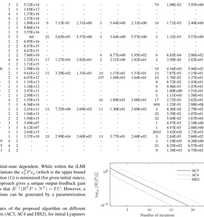
Convergence rates of the proposed algorithm on different COMPleib plants (AC3, AC4 and DIS2), for initial Lyapunov matrices obtained from standard state-feedback LQR design, are shown in Fig. 1. Convergence rates of the proposed algorithm on the COMPleib plant AC3 for random initial Lyapunov matrices are shown in Fig. 2. From figures follow that the convergence rate is linear if the initial Lyapunov matrix is calculated by the standard LQR design, and that it becomes linear in the neighbourhood of the solution.

V. CONCLUSIONS

A novel iterative design is proposed for output-feedback LQR design for LTI systems with guaranteed convergence to a solution (for an initial Lyapunov matrix obtained for any stabilizing state-feedback gain). Numerical results highlight that the proposed approach is computationally much more tractable then approaches based on LMIs and/or BMIs. Along this line, numerical results also indicate that regu-larization is needed to improve usability of the proposed approach for ill-conditioned problems. This can be done by preconditioning the Lyapunov equation within the Newton’s

5 10 15 20 Number of iterations 10-10 100 AC3 AC4 DIS2

Fig. 1. Convergence rate of the Algorithm 1 on COMPleib plants AC3,

AC4 and DIS2. The initial Lyapunov matrix is obtained by the standard state-feedback LQR design.

10 20 30 40 50 60 70

Number of iterations 10-10

100

Fig. 2. Convergence rate of the Algorithm 1 on COMPleib plant AC3 for

method similarly as in [32]. Furthermore, the proposed approach can be easily extended with exact line-search, similarly as it is done in [29] to speed up the convergence. Finally, using a technique introduced in [43], a robust output-feedback controller can be designed by the proposed approach.

REFERENCES

[1] H. Kwakernaak and R. Sivan,Linear optimal control systems. Wiley-Interscience, 1972.

[2] J. Willems, “Least squares stationary optimal control and the algebraic riccati equation,”IEEE Transactions on Automatic Control, vol. 16, no. 6, pp. 621–634, Dec 1971.

[3] B. Molinari, “The time-invariant linear-quadratic optimal control prob-lem,”Automatica, vol. 13, no. 4, pp. 347 – 357, 1977.

[4] H. L. Trentelman and J. C. Willems,The Dissipation Inequality and the Algebraic Riccati Equation. Berlin, Heidelberg: Springer Berlin Heidelberg, 1991, pp. 197–242.

[5] V. Syrmos, C. Abdallah, P. Dorato, and K. Grigoriadis, “Static output feedback–A survey,”Automatica, vol. 33, no. 2, pp. 125–137, 1997. [6] M. Sadabadi and D. Peaucelle, “From Static Output Feedback to

Structured Robust Static Output Feedback: A Survey,”Annual Reviews in Control, vol. 42, pp. 11–26, 2016.

[7] D. Moerder and A. Calise, “Convergence of a numerical algorithm for calculating optimal output feedback gains.”IEEE Transactions on Automatic Control, vol. 30, pp. 900–903, 1985.

[8] V. Kuˇcera and C. E. De Souza, “A necessary and sufficient conditions for output feedback stabilizability,” Automatica, vol. 31, no. 9, pp. 1357–1359, 1995.

[9] T. Iwasaki, R. Skelton, and J. Geromel, “Linear quadratic suboptimal control with static output feedback,” Systems ad Control Letters, vol. 23, pp. 421–430, 1994.

[10] V. Vesel´y and A. Ilka, “Gain-scheduled PID controller design,”Journal of Process Control, vol. 23, no. 8, pp. 1141–1148, Sept. 2013. [11] V. Vesel´y, “Static output feedback controller design,” Kybernetica,

vol. 37, no. 2, pp. 205–221, 2001.

[12] J. Engwerda and A. Weeren, “A result on output feedback linear quadratic control,”Automatica, vol. 44, no. 1, pp. 265–271, 2008. [13] V. Vesel´y, “Static output feedback robust controller design via LMI

approach,”Journal of Electrical Engineering, vol. 56, no. 1-2, pp. 3–8, 2005.

[14] ——, “Robust controller design for linear polytopic systems,” Kyber-netika, vol. 42, no. 1, pp. 95–110, 2006.

[15] D. Rosinov´a and V. Vesel´y, “Robust PID decentralized controller design using LMI,” International Journal of Computers, Communi-cations & Control, vol. 2, no. 2, pp. 195–204, 2007.

[16] V. Vesel´y and A. Ilka, “Design of robust gain-scheduled PI con-trollers,”Journal of the Franklin Institute, vol. 352, no. 4, pp. 1476 – 1494, 2015.

[17] A. Ilka, “Matlab/Octave toolbox for structurable and robust output-feedback LQR design,”IFAC-PapersOnLine, vol. 51, no. 4, pp. 598 – 603, 2018, 3rd IFAC Conference on Advances in Proportional-Integral-Derivative Control PID 2018.

[18] V. Vesel´y and D. Rosinov´a, “Robust PID-PSD Controller Design: BMI Approach,” Asian Journal of Control, vol. 15, no. 2, pp. 469–478, 2013.

[19] A. Ilka and V. Vesel´y, “Gain-Scheduled Controller Design: Variable Weighting Approach,” Journal of Electrical Engineering, vol. 65, no. 2, pp. 116–120, March-April 2014.

[20] V. Vesel´y and A. Ilka, “Generalized robust gain-scheduled PID con-troller design for affine LPV systems with polytopic uncertainty,”

Submitted to Systems and Control Letters, vol. 0, no. 0, pp. 0–0, 2016. [23] H. Toivonen, “A globally convergent algorithm for the optimal constant output feedback problem,”International Journal of Control, vol. 41, pp. 1589–1599, 1985.

[21] A. Ilka and V. Vesely, “Robust LPV-based infinite horizon LQR design,” in2017 21st International Conference on Process Control (PC), June 2017, pp. 86–91.

[22] ——, “Robust guaranteed cost output-feedback gain-scheduled con-troller design,” IFAC-PapersOnLine, vol. 50, no. 1, pp. 11 355 – 11 360, 2017, 20th IFAC World Congress.

[24] D. Moerder and A. Calise, “Convergence of a numerical algorithm for calculating optimal output feedback gains,”IEEE Transactions on Automatic Control, vol. 30, pp. 900–903, 1985.

[25] E. J. Davison, N. S. Rau, and F. V. Palmay, “The optimal decentralized control of a power system consisting of a number of interconnected synchronous machines,” International Journal of Control, vol. 18, no. 6, pp. 1313–1328, 1973.

[26] D. Petersson and J. L¨ofberg, “LPV H2-controller synthesis using nonlinear programming,” in Proceedings of the 18th IFAC World Congress, 2011.

[27] K. Zhou, C. J. Doyle, and K. Glover,Robust and optimal control. Prentice-Hall, Inc., Upper Saddle River, NJ, USA, 1996.

[28] W. M. Wonham, Linear Multivariable Control: A Geometric Ap-proach, 3rd ed. New York: Springer-Verlag, 1985.

[29] P. Benner and R. Byers, “Newton’s method with exact line search for solving the algebraic riccati equation,” IEEE Transactions on Automatic Control, vol. 43, pp. 101–107, 1998.

[30] C. Guo and A. Laub, “On a Newton-Like Method for Solving Algebraic Riccati Equations,”SIAM Journal on Matrix Analysis and Applications, vol. 21, no. 2, pp. 694–698, 2000.

[31] C.-H. Guo and A. J. Laub, “On a Newton-like method for solving algebraic Riccati equations,” SIAM Journal on Matrix Analysis and Applications, vol. 21, no. 2, pp. 694–698, 2000.

[32] J.-P. Chehab and M. Raydan, “Inexact Newton’s method with inner im-plicit preconditioning for algebraic Riccati equations,”Computational and Applied Mathematics, vol. 36, pp. 955–969, 2017.

[33] M. Dehghan and M. Hajarian, “Construction of an iterative method for solving generalized coupled Sylvester matrix equations,”Transactions of the Institute of Measurement and Control, vol. 35, no. 8, pp. 961– 970, 2013.

[34] M. Hajarian, “Extending the CGLS algorithm for least squares solu-tions of the generalized Sylvester-transpose matrix equasolu-tions,”Journal of the Franklin Institute, vol. 353, no. 5, pp. 1168 – 1185, 2016, special Issue on Matrix Equations with Application to Control Theory. [35] ——, “Finite algorithms for solving the coupled Sylvester-conjugate

matrix equations over reflexive and Hermitian reflexive matrices,”

International Journal of Systems Science, vol. 46, no. 3, pp. 488–502, 2015.

[36] P. Lancester and M. Tismenetsky,The Theory of Matrices, 2nd ed. Orlando: Academic Press, 1985.

[37] F. Leibfritz, “COMPleib: COnstraint Matrix-optimization Problem library - a collection of test examples for nonlinear semidefinite programs, control system design and related problems.” University of Trier, Department of Mathematics, D54286 Trier, Germany, Tech. Rep., 2004.

[38] The Mathworks, Inc.,MATLAB R2017a, The Mathworks, Inc., Natick, Massachusetts, 2017.

[39] J. Fiala, M. Koˇcvara, and M. Stingl, “Penlab: A matlab solver for nonlinear semidefinite optimization,” October 2013, submitted to Mathematical Programming Computation.

[40] MOSEK Optimization Toolbox for MATLAB, MOSEK ApS, 2018. [41] J. L¨ofberg, “ YALMIP : A Toolbox for Modeling and Optimization in

MATLAB,” inProceedings of the CACSD Conference, Taipei, Taiwan, 2004.

[42] R. E. Skelton and T. Iwasaki, “Lyapunov and covariance controllers,”

International Journal of Control, vol. 57, pp. 519–536, 1993. [43] F. Lin, “An optimal control approach to robust control design,”