Volatility Forecasting in Commodity
Markets using Macro Uncertainty
Dimitrios Bakas
a,c †and
Athanasios Triantafyllou
b aNottingham Business School, Nottingham Trent University, UKbEssex Business School, University of Essex, UK cRimini Centre for Economic Analysis (RCEA), Canada
Abstract
In this paper, we empirically examine the predictive power of macroeconomic uncertainty on the volatility of agricultural, energy and metals commodity markets. We find that the latent macroeconomic uncertainty measure of Jurado et al. (2015) is a common volatility forecasting factor for commodity markets, which provides statistically significant volatility predictions for forecasting horizons up to twelve months ahead. The results indicate that the forecasting power of macroeconomic uncertainty is higher when predicting the volatility of energy commodities. Our findings also show that higher macroeconomic uncertainty is associated with large volatility episodes subsequently observed in all commodity markets. The predictive power of the unobservable macroeconomic uncertainty factor remains robust to the inclusion of observable economic uncertainty measures, historical commodity price volatility, stock-market realized and news implied volatility, oil price shocks and other macroeconomic variables which are closely related to the production process and the mechanics of commodity markets.
Keywords:Commodity Markets,Volatility, Macroeconomic Uncertainty, Forecasting
JEL Classification:C22, E32, G13, O13, Q02
†Acknowledgments: We would like to thank an anonymous referee for the constructive comments
and helpful suggestions. In addition, we would like to thank the participants of the 2017 Paris Financial Management Conference(PFMC-2017) for their useful comments and suggestions. Any remaining errors are the responsibility of the authors. The authors declare that they have no conflict of interest.
Corresponding author: Dimitrios Bakas, Nottingham Business School, Nottingham Trent University, 50 Shakespeare Street, Nottingham, NG1 4FQ, United Kingdom.
1
1. Introduction
Co-movements in commodity markets occur quite frequently, especially in the post-financialization era. Many empirical studies identify the existence of significant co-movements in commodity markets (Batten et al., 2010; Pindyck and Rotemberg, 1990; Frankel and Rose, 2010; among others), but fail to attribute this characteristic to macroeconomic factors. For example, Batten et al. (2010) find that there are no common macroeconomic factors influencing volatility dynamics in metals commodity markets, while Pindyck and Rotemberg (1990), by examining the ‘excess co-movement’ hypothesis of commodity prices, show that these co-movements are well in excess of anything that can be explained by common macroeconomic factors like inflation and exchange rates. On the other hand, Frankel and Rose (2010) suggest that there are times during which almost all commodity prices move together, so it is difficult to ignore the macroeconomic factors when searching for the determinants of commodity prices. While there are many empirical studies showing the impact of macroeconomic and monetary factors on commodity prices (Anzuini et al., 2013; Frankel, 2008; Frankel and Hardouvelis, 1985; Frankel and Rose, 2010; Gilbert, 2010; Gordon and Rowenhorst, 2006; Gubler and Hertweck, 2013; Hammoudeh et al., 2015; Triantafyllou and Dotsis, 2017), the linkages between the macroeconomy and the volatility in commodity markets have not yet been extensively examined. In addition, the literature on the modeling and forecasting of commodity markets volatility has indicated both long-memory and persistence of volatility dynamics as notable characteristics of commodity markets (Agnolucci, 2009; Chkili et al., 2014; among others), however, it has remained silent on the common macroeconomic factors that drive the persistence and the common variation in the volatility of commodity markets.
While many empirical studies show that the heightened macroeconomic uncertainty signficantly reduces stock-market returns and increases the volatility on equity markets (Antonakakis et al., 2013; Arouri et al., 2016; Kang and Ratti, 2014; Kelly et al., 2016; Ozoguz, 2008; among others), there are only few recent empirical applications showing the impact of macroeconomic uncertainty shocks on commodity markets, and particularly, on the volatility of commodity prices (Bakas and Triantafyllou, 2018; Christoffersen et al., 2018; Joëts et al., 2017; Nguyen and
2
Walther, 2018; Smales, 2017; Van Robays, 2016; Wei et al., 2017). For instance, Smales (2017) shows that volatility in commodity markets is significantly impacted by U.S. and Chinese macroeconomic news which reveal information about aggregate demand for commodities, while Van Robays (2016) shows that the higher macroeoconomic uncertainty, as measured by the volatility of aggregate U.S. industrial production, has a significant positive impact on volatility of oil prices. In addition, Christoffersen et al. (2018) show that commodity price volatility displays a significant degree of integration across commodity markets and that the common factors which drive the joint dynamics in commodity volatility are related to business cycles and stock-market volatility. Lastly, the paper of Joëts et al. (2017), which is the closest work to ours, investigates the impact of macroeconomic uncertainty on commodity price returns and volatility, and shows that the commodities which are more sensitive to macroeconomic uncertainty are the agricultural and industrial markets.
Motivated by these empirical findings, which identify a significant impact of uncertainty shocks on commodity market volatility, we contribute to the literature by examine empirically the forecasting power of macroeconomic uncertainty on the volatility in commodity prices.1 In this way, our paper extends previous studies, such
as Van Robays (2016) and Joëts et al. (2017), by examining the predictive power of macroeconomic uncertainty for a panel of commodities. We show that the unobservable macroeconomic uncertainty measure of Jurado et al. (2015) (JLN hereafter) is the most significant and robust common volatility forecasting factor for commodity markets.2 The JLN macroeconomic uncertainty factor produces
statistically significant forecasts when forecasting the volatility in agricultural, energy and metals commodity markets, with the forecasting horizon ranging from one to
1 Our paper also contributes to the empirical works that study the economic drivers of financial volatility. Starting with Schwert (1989), a large body of literature explores the various financial and macroeconomic predictors of volatility in financial markets (e.g., Christiansen et al., 2012; Feng et al., 2017; Paye, 2012; Wang et al., 2018). The previous literature mainly focuses on either the stock market volatility or the volatility of energy commodities. In this paper, we examine the impact of macroeconomic uncertainty on the volatility of a broad class of agricultural, energy and metals commodity markets.
2The unobservable JNL macroeconomic uncertainty factor provides the most statistically significant forecasts and contains all the predictive information content which is already included in observable proxies of macroeconomic and financial uncertainty that are based on macroeconomic or financial news (e.g., the economic policy uncertainty measure of Baker et al. (2016) or the news implied volatility index of Manela and Moreira (2017)).
3
twelve months. The predictive power of macroeconomic uncertainty is higher in energy commodities like crude oil and gasoline. These findings provide further robustness to the oil-macroeconomy relationship (Hamilton, 2003; Elder and Serletis, 2010; Kilian and Vigfusson, 2017; among others), according to which rising oil prices and volatility cause economic recessions, since we show a reverse type of causality where rising macroeconomic uncertainty is a singificant indicator of turbulence in oil markets. Our results remain robust for both in-sample and out-of-sample forecasts, and also when controlling for alternative observable economic uncertainty factors, such as the economic policy uncertainty (Baker et al., 2016), the stock-market realized volatility (Bloom, 2009) and the news implied financial volatility (Manela and Moreira, 2017), as well as for the persistence of commodity market volatility (by including the lagged volatility in the information variable set), the crude oil price shocks (Hammoudeh and Yuan, 2008; Wang et al., 2014) and several other macroeconomic factors which are directly related with commodity volatility dynamics. The predictive regression models show that the macroeconomic uncertainty (MU) factor alone is capable of displaying significant commodity volatility forecasts, with the R2 values reaching almost 30% for both in-sample and out-of-sample forecasts. In addition, the MU factor provides better commodity volatility predictions for in-sample and out-of-sample estimations when compared with the benchmark AR models. Furthermore, the bivariate regression model which includes the MU factor as the only predictor of commodity market volatility, provides more significant real time (out-of-sample) forecasts when compared with the respective performance of the multivariate models and outperforms the benchmark autoregressive volatility forecasting modelsin the out-of-sample evaluation period. Lastly, the estimated DCC-GARCH model shows that the time-varying conditional covariance between macroeconomic uncertainty and volatility in commodity prices remains positive during all the period under investigation and increases significantly over the recent period of the 2007-2009 financial crisis, during which the overall uncertainty in the macroeconomy has increased exponentially.
Our findings, for the first time in the literature, identify the robust forecasting power of the JLN macroeconomic uncertainty measure on the volatility of energy, metals and agricultural commodity futures returns, and indicate that rising macroeconomic uncertainty is followed by large and persistent commodity volatility episodes in all
4
major (agricultural, energy and metals) commodity markets. Our primary contribution in the literature, is that we provide evidence that the latent macroeconomic uncertainty measure of JLN (which quantifies the degree of unepredictability regarding the future state of the macroeconomy) is the most significant common volatility forecasting (macroeconomic) factor for the commodity markets. In this respect, our results confirm the evidence of Joëts et al. (2017), who show that most of the commodity markets are affected by macroeconomic uncertainty, while extend the evidence of Delle Chiaie et al. (2017), who demonstrate that fluctuations in commodity prices are driven by a single (latent) factor, by presenting that the latent MU indicator is a robust common factor for commodity markets volatility. Furthermore, our findings, in contrast with Wei et al. (2017), who identify the observable economic policy uncertainty index as the most informative determinant of crude oil market volatility, and Liu et al. (2018), who find that the news implied financial volatility index is a significant determinant for the volatility of non-energy markets, show that the unobservable MU factor exhibits higher predictive power for a broad class of commodity markets (agricultural, energy and metals), and absorbs all the predictive information of the observable macroeconomic and financial uncertainty indexes. Our evidence, in simple words, reveals that the most significant macroeconomic determinant which drives volatility in commodity markets is a latent factor and it cannot be related to any observable economic fluctuations. The robust forecasting power of the JLN macroeconomic uncertainty factor represents the first purely macroeconomic explanation for the Pindyck and Rotemberg (1990), and recently discussed in Ohashi and Okimoto (2016), phenomenon of a puzzling and unexplainable (by macroeconomic fundamentals) ‘excess co-movement’ in commodity markets. The economic interpretation of our results is that the most significant early warning signal for large volatility episodes in commodity markets cannot be related to changes in agreggate demand and aggregate industrial production, but to the rising degree of uncertainty (or unpredictability) in the macroeconomy, which, thus, can be interpreted as the unforeseeable path of macroeconomic fluctuations, and consequently, the unforeseeable changes in agreggate demand for commodities.
5
The rest of the paper is organized as follows. Section 2 describes the data. Section 3
presents the empirical results and provides robustness checks. Finally, Section 4
concludes.
2. Data
For our empirical analysis, we use the daily S&P GSCI commodity futures prices. In specific, we use 12 individual daily time series for excess returns for agricultural, energy and metals commodities based on the S&P GSCI commodity futures market index. The group of agricultural commodities includes corn, cotton, soybeans and wheat, while the group of energy commodities includes crude oil, heating oil, petroleum and gasoline, and finally, the group of metals commodities includes copper, gold, platinum and silver. We employ a balanced dataset for the 12 commodities that covers the period from January 1988 to December 2016. All daily S&P GSCI series were downloaded from Datastream.
To construct the monthly realized variance we follow the empirical approach of Christensen and Prabhala (1998) and Wang et al. (2012) and estimate the realized variance as the monthly variance of the daily returns of commodity futures as follows:
2 1 1 , 1 1 1 1 T t i t i t i t i t T i t i t i F F F F RV T F F + + − + + − = + − + − − − = −
, (1)where Ft is the commodity futures price for trading day t and the time interval [t,T] is the number of trading days during each monthly period. 𝑅𝑉𝑡,𝑇 is the measure of the estimated realized variance for each month.
The measure of the unobservable (latent) macroeconomic uncertainty (MU) is based on the work of Jurado et al. (2015). The JLN MU uncertainty index is measured as the purely unforecastable (by economic agents) part of macroeconomic fluctuations. More specifically, the latent macroeconomic uncertainty is defined in Jurado et al. (2015) as the purely unforcastable component of the future path of macroeconomic series, which is given by:
6
uj t,( )h = E Y( j t h,+ −E Y[ j t h,+ ]) It 2 It , (2)
where Yjt+h is the actual value of a macroeconomic variable Yj after h periods (months) from the current month t, while E Y[ j t h,+ ]It is the conditional expectation (given all the information (It) available to economic agents at time t) about the future price of the macroeconomic time series, Yj, h periods ahead. The macroeconomic uncertainty (MU) index is then constructed as the aggregation of the individual uncertainty measures, uj t,( )h , in each monthly period t, using some aggregation weights (wj)
which are proportional to the significance of each variable Yj for the macroeconomy, as u ht( )=E uw[ j t,( )]h . According to this approach, the macroeconomic uncertainty measure does not nessecarily coincide with popular uncertainty proxies based on observable volatility since the financial markets and the macroeconomic indicators may fluctuate for reasons which are not related to uncertainty.3 In our analysis, we use the logarithm of the 3-months ahead (h=3) macroeconomic uncertainty measure of Jurado et al. (2015) which corresponds to the time varying uncertainty for the US macroeconomy when having 3-month forecasting horizon. The JLN MU measure is downloaded from Sydney Ludvigson’s webpage.
We also use data for the measure of observable economic uncertainty which is based on macroeconomic news. More specifically, we use the logarithm of the economic policy uncertainty (EPU) series based on the approach of Baker et al. (2016), according to which the economic uncertainty is proxied by uncertainty about economic policy which can be observed in economic news and newspaper articles. We obtain the EPU index from http://www.policyuncertainty.com. Additionally, we use the realized variance of the daily returns of the S&P 500 stock-market index (SP500RV) as another proxy of economic uncertainty which is based on the fluctuations of observable equity market prices (Bloom, 2009). The daily series of the S&P 500 index (SP500) were downloaded from Datastream.4 Lastly, we use the news implied volatility (NVIX) series of Manela and Moreira (2017), which is a text-based
3Jurado et al. (2015) suggest, for example, that stock-market volatility can change over time even if there is no change in uncertainty about economic fundamentals, if leverage changes, or if movements in risk aversion or sentiment are important drivers of asset market fluctuations.
4The realized variance (SP500RV) of the S&P 500 index has been estimated by employing the same methodology as in Equation (1).
7
measure of uncertainty that focuses on investors’ concerns as covered in front-page articles of the Wall Street Journal. The NVIX measure is downloaded from Asaf Manela’s webpage.
We finally obtain monthly data on various macroeconomic time-series which have been proposed as significant determinants for commodity markets. We include the logarithm of the oil price (OILP), the rate of inflation (INFL), the logarithm of the U.S. effective exchange rate (EXCH), and the slope of the term structure (or term spread) based on the difference between the 10-year U.S. government bond yield and the 3-month U.S. Treasury Bill rate (TERM). All macroeconomic time-series were downloaded from FRED.5
3. Empirical Results and Robustness Checks
3.1 Descriptive StatisticsIn this section we report the descriptive statistics for the 12 commodity volatility series and the macroeconomic and uncertainty indicators which are used as volatility forecasting factors. The cross-section of the 12 commodities used in our analysis consists the following: corn, cotton, soybeans, wheat (agricultural), crude oil, heating oil, petroleum, gasoline (energy), and copper, gold, platinum, silver (metals). Table 1
shows the descriptive statistics for the commodity realized volatility series and the macroeconomic and uncertainty variables.
[Insert Table 1 Here]
More specifically, the average value of the monthly realized variance is about 0.06 for most agricultural and metals commodity prices like the corn, wheat, soybeans, platinum and silver, while for the energy commodity futures returns the realized variance is significantly higher (about 0.11). In addition, the mean value of MU and EPU series (which quantify the unobservable and the observable macroeconomic uncertainty shocks respectively) is nearly the same.6,7 Furthermore, we report in
5 All series have monthly frequency and cover the period from January 1988 until December 2016, except the NVIX index for which the data ends in March 2016.
6 The MU uncertainty series have been multiplied by 100 in order to be directly comparable to the economic policy uncertainty (EPU) series.
8
Table 2 the correlation coefficients between the agricultural, energy and metals
commodity series.
[Insert Table 2 Here]
From Table 2 we observe that the commodity variance series are highly correlated with the correlation coefficients being positive and more than 35% for all alternative commodity volatility series. The volatility series exhibit higher correlation for those commodities that belong to the same commodity group, compared to the correlation coefficients of commodities that belong to a different commodity groups. This evidence is in line with the empirical findings of Christoffersen et al. (2018) who show that for the post-financialization era, commodity market volatily displays a significant degree of integration across the various classes of commodities.
Lastly, we present the contemporaneous time series evolution of the macroeconomic uncertainty measure and the series of the monthly realized variance in the three groups of our commodity futures returns. Figure 1, 2 and 3 plot the contemporaneous movements between the time series of the MU and the realized variance of agricultural, energy and metals markets respectively.
[Insert Figure 1 Here] [Insert Figure 2 Here] [Insert Figure 3 Here]
From Figures 1, 2 and 3 we can observe that high level of macroeconomic uncertainty is associated with a subsequent rise in the volatility for all commodity markets under consideration. This evidence can be interpreted as a first empirical observation that the MU measure is a significant early warning signal of commodity market volatility episodes. The plots in Figures 1-3 clearly show that the heightened uncertainty in the 2007-2009 period coincides with significant jumps in the volatility of all commodity prices. Finally, Figure 4 shows the evolution of the alternative measures of economic uncertainty, namely the macroeconomic uncertainty (MU), the
7All explanatory variables have been tested for stationarity and the null hypothesis of unit root have been rejected using both the Augmented Dickey-Fuller and the Philips-Perron unit root tests. For brevity, we do not report the results here, but they are provided upon request.
9
economic policy uncertainty (EPU), the realized volatility of the S&P 500 index (SP500RV) and the news implied volatility (NVIX). We can observe the synchronization of the uncertainty measures during certain episodes (e.g., the crisis period), however the comovement among the measures and their responsiveness to various episodes vary over time. In addition, we observe that jumps in MU series occur less frequently in comparison to jumps in other proxies of economic uncertainty, but they are more persistent when occuring. The persistent and infrequent nature of macroeconomic uncertainty episodes coincides (according to Figures 1-3) with the rising volatility in commodity markets.
[Insert Figure 4 Here]
3.2 In-sample Forecasting Regression Models
We start by presenting the estimations of the bivariate OLS forecasting regression models in which we use the MU series as the only predictor of the monthly volatility in commodity futures returns.8 The bivariate time-series regression model is given in
Equation (3) below:
0 1
t t k t
RV = +b b MU− + , (3)
where RV is the realized variance of the commodity futures returns and MU is the JLN macroeconomic uncertainty. The forecasting horizon ranges from 1 to 12 months. Table 3, 4 and 5 report the bivariate regression results when forecasting the volatility of the agricultural (corn, cotton, soybeans and wheat), energy (crude oil, heating oil, petroleum and gasoline) and metals (copper, gold, platinum and silver) commodity futures prices respectively.
[Insert Table 3 Here] [Insert Table 4 Here]
8The focus of our empirical analysis is on the forecasting power of the unobservable macroeconomic uncertainty measure of Jurado et al. (2015) (namely the MU series). Bakas and Triantafyllou (2018) by examining empirically the response of commodity volatility on several other alternative economic uncertainty measures (like the EPU economic uncertainty measure and its components and the VXO stock-market uncertainty index among others) verify that all observable measures of macroeconomic and financial uncertainty do not contain any superior information compared to the MU series.
10
[Insert Table 5 Here]
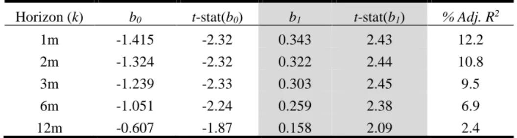
From Tables 3-5 we observe that the coefficient of the MU factor remains positive and statistically significant for all forecasting horizons ranging from 1 to 12 months for all the commodity markets under investigation. The estimated coefficients of the MU factor, when is used as predictor for energy commodities are significantly larger (i.e., more than 3 times) when compared to the estimated coefficients in agricultural and metals commodity markets. For example, the estimated MU coefficients when forecasting the one-month ahead volatility of crude oil, petroleum and gasoline (energy) are approximately 0.73, 0.60 and 0.70 respectively, while the respective coefficients for corn, cotton and soybeans (agricultural), as well as for gold, platinum and silver (metals) volatility forecasts are approximately 0.25, 0.22, 0.17 and 0.15, 0.25 and 0.34 respectively. In addition, the forecasting power of the MU factor slightly deteriorates when we lenghten the forecasting horizon. For example, the R2of the predictive regressions is 18% and drops to 16.3% when we forecast the corn futures volatility having one-month and six-month horizon respectively.9 The estimated MU coefficients when forecasting the volatility in crude oil and petroleum markets are significantly larger when compared to those of the other commodity markets. These results extend the recent empirical findings of Delle Chiaie et al. (2017) who identify a single global macroeconomic (latent) factor behind commodity prices fluctuations, by suggesting that the latent MU measure of JLN is the most significant and robust common forecasting factor for commodity markets volatility, and are in line with Nguyen and Walther (2018), who find that the long-term volatility component in commodity markets is driven by macroeconomic factors like global real economic activity and economic policy uncertainty, and Joëts et al. (2017), who suggest that macroeconomic uncertainty significantly affects volatility in commodity markets. Furthermore, while Wei et al. (2017) present that the EPU measure is a significant determinant of crude oil market volatility and Liu et al. (2018) that the NVIX index is a significant determinant for non-energy commodities volatility, we show that the unobservable JLN MU factor is a significant predictor for a broad class of agricultural, energy and metals commodity markets, and that this factor absorbs all the predictive power of the observable EPU and NVIX uncertainty indexes. Our
9 The R2 value reported in our results is the adjusted R2 (in percentages) which controls for the number
11
results regarding the significance and the predictive power of macroeconomic uncertainty on oil price volatility are in line and give further empirical support to the relevant literature which identify the impact of oil price and uncertainty shocks on the macroeconomy (Elder, 2018; Elder and Serletis, 2010; Hamilton, 2003; Jo, 2014; Kilian, 2008; Rahman and Serletis, 2011). Our empirical analysis contributes to the relevant literature by revealing a reverse channel of causality, since our results shows that the macroeconomic uncertainty shocks are the key driver and the common (latent) factor driving the time varying volatility in oil markets. In simple words, our empirical findings reveal a bi-directional linkage between the macroeconomic uncertainty shocks and fluctuations and the oil market turbulances.
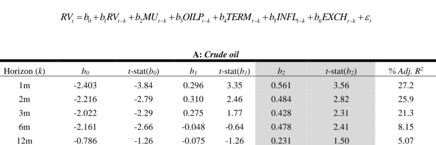
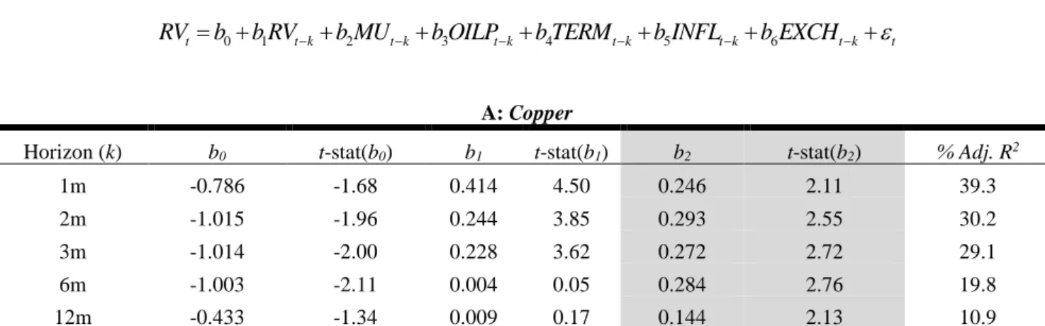
Moreover, in order to provide robustness to the previous empirical findings, we employ a multivariate regression model in which we include some of the already empirically verified macroeoconomic determinants of commodity price and volatility dynamics (OILP, INFL, EXCH) on the left-hand side of the predictive regression equation (Beckerman and Jenkinson, 1986; Chen et al., 2010; Frankel and Rose, 2010; Gilbert, 2010; Gordon and Rowenhorst, 2006; Gospodinov and Ng, 2013; Hammoudeh and Yuan, 2008;Lizardo and Mollick, 2010). Furthermore, motivated by the findings in the relevant literature which show that commodity markets are significantly affected by monetary policy and interest rates (Akram, 2009; Anzuini et al., 2013; Frankel, 2008; Frankel and Hardouvelis, 1985; Gubler and Hertweck, 2013; Hammoudeh et al., 2015; Triantafyllou and Dotsis, 2017), we additionally include the term spread (TERM) into the information variable set. In addition, and in order to control for the persistence of the commodity volatility series (see for example, Elder and Jin, 2007; Vivian and Wohar, 2012; Chkili et al., 2014) we include the lagged realized variance as an additional predictor of future variance. The multivariate time-series regression model, where we control for macroeconomic fundamentals, is given
in Equation (4) below:
0 1 2 3 4 5 6
t t k t k t k t k t k t k t
RV = +b b RV− +b MU− +b OILP− +b TERM− +b INFL− +b EXCH− +
,(4) where RV is the realized variance of the commodity futures returns, MU is the JLN macroeconomic uncertainty, RVt-k is the lagged realized variance and OILP, INFL,12
EXCH and TERM are the macroeconomic controls. The forecasting horizon ranges from 1 to 12 months. The results of the multivariate regression model are given in
Tables 6, 7 and 8.
[Insert Table 6 Here] [Insert Table 7 Here] [Insert Table 8 Here]
In Tables 6-8, RV is the lagged realized variance, MU is the logarithm of the JLN
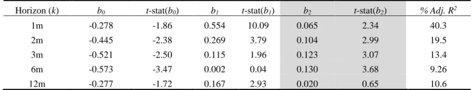
macroeconomic uncertainty, OILP is the logarithm of the crude oil price, TERM is the term spread, INFL is the inflation rate and EXCH is the logarithm of the U.S. effective exchange rate.10 The results from Tables 6-8 show that the predictive ability of the MU factor remains robust to the inclusion of various traditional macroeconomic determinants of commodity prices, like the crude oil price, the U.S. effective exchange rate, the term spread and the inflation rate. Furthermore, the predictive power of the MU factor remains unchanged when we control for the persistence of commodity market volatility by including the lagged volatility into the predictive regression models.
More specifically, the estimated MU coefficients, under the multivariate predictive regression specification that controls for macroeoconomic fundamentals, remain positive and statistically significant for 1 up to 6-months forecasting horizons in all commodities except silver. On the other hand, the coefficients of the lagged realized variance remain significant for 1 up to 3-months forecasting horizons, while for the 6-months and 12-6-months horizons the coefficients become insignificant for most of the commodities examined (9 out of 12 commodities). These results show that the unobservable MU factor can capture both the time series dynamics and the persistence of commodity volatility, since we observe that for longer-term (more than 3-months) forecasting horizons, the MU factor absorbs all predictive power of the lagged realized variance.
10For brevity, in Tables 6-8 and 9-11 we report only the coefficients of MU (b
2) and of the lagged
13
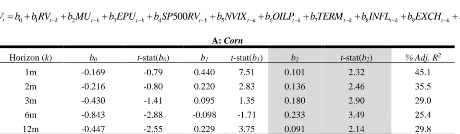
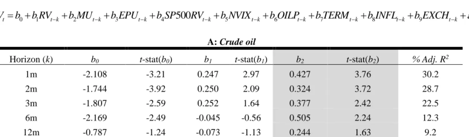
We extend our previous robustness check by using a multivariate regression model that controls for both macroeconomic and economic uncertainty factors. Following the literature on the association of uncertainty with commodity markets volatility (Bakas and Triantafyllou, 2018; Joëts et al., 2017; Liu et al., 2018; Wei et al., 2017; among others), we include several alternative proxies of economic uncertainty to examine the predictive power of the MU factor when allowing for other measures of uncerainty in the regression. Specifically, in addition to the above macroeconomic factors (OILP, INFL, EXCH, TERM), we use the economic policy uncertainty measure (EPU) of Baker et al. (2016) that accounts for observable macroeconomic uncertainty. In order to control for the volatility spillover effect from equity to commodity markets (see Diebold and Yilmaz, 2012), we include the realized variance of the S&P 500 stock-market index (SP500RV) into the variable information set. Lastly, we use the news implied volatility index (NVIX) of Manela and Moreira (2017) that is a text-based observed measure of financial uncertainty (see Su et al., 2018). The multivariate time-series regression model, where we control for both macroeconomic fundamentals and alternative economic uncertainty measures, is given in Equation (5) below:
0 1 2 3 4 5 6 7 8 9 500 t t k t k t k t k t k t k t k t k t k t RV b b RV b MU b EPU b SP RV b NVIX
b OILP b TERM b INFL b EXCH
− − − − −
− − − −
= + + + + +
+ + + + + , (5)
where RV is the realized variance of the commodity futures returns, MU is the JLN macroeconomic uncertainty, RVt-k is the lagged realized variance, OILP, INFL, EXCH and TERM are the macroeconomic controls and EPU, SP500RV and NVIX are the additional economic uncertainty measures. The forecasting horizon ranges from 1 to 12 months. The results of the multivariate regression model, that controls for both macroeconomic and uncertainty factors, for the agricultural, energy and metals commodity markets are given in Tables 9, 10 and 11.
[Insert Table 9 Here] [Insert Table 10 Here] [Insert Table 11 Here]
14
In Tables 9-11, in addition to the macroeconomic variables that we use in the
multivariate model presented in Tables 6-8,we include EPU, that is the logarithm of economic policy uncertainty, SP500RV, that is the realized variance of the S&P 500 index and NVIX, that is the logarithm of the news implied volatility series. This robustness test helps us to check whether the forecasting power of the MU factor is affected by the other measures of observed economic uncertainty. The results from
Tables 9-11 show that the predictive ability of the MU factor remains robust to the
inclusion of observable economic uncertainty measures, like the EPU and the NVIX indexes. More specifically, the estimated coefficients of the MU factor and the respective R2values of the predictive regressions change only marginally when the alternative economic uncertainty proxies are added on the left-hand side of the regression equation.
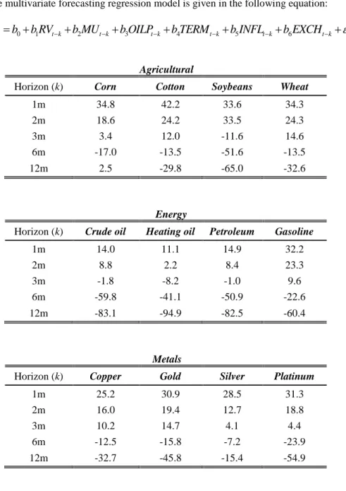
3.3 Out-of-sample Forecasting Regression Models
In order to check for the robustness of the goodness-of-fit of our forecasting regression models, we estimate out-of-sample forecasts for the period t+h (where h is the forecasting horizon) using available data up to t months. We use an initial time series window of 60 months and run the regressions in order to forecast the monthy realized variance of commodity prices t+h months ahead. The estimation window is then extended by one monthly period in order to obtain a new out-of-sample forecast. We use the same bivariate and multivariate forecasting regression models as described in Section 3.2 (provided in Equations 3-5) and create dynamic out-of-sample forecasts and compute the respective out-of-out-of-sample R2 values.11 The out-of-sample R2 values for the bivariate and multivariate regression models are given in
Tables 12, 13 and 14 respectively.
[Insert Table 12 Here] [Insert Table 13 Here] [Insert Table 14 Here]
11 Following the previous empirical literature (Christiansen et al., 2012; Paye, 2012; Wang et al., 2018), we use the out-of-sample 𝑅2 to evaluate the out-of-sample performance of our models.
15
The out-of-sample forecasting evidence shows that the predictive power of the MU factor remains practically unaffected for both short and medium-term forecasting horizon (for 1 up to 6 months ahead). For example, the out-of-sample R2 value is 19.8%, 15.3% and 14.8% when estimating the dynamic out-of-sample forecasts for the one-month ahead volatility for gold, crude oil and corn futures returns respectively. Interestingly, when comparing the out-of-sample goodness of fit for the bivariate and multivariate regression models, we can see that the respective R2 values are significantly larger for the bivariate model, in most of the commodity markets. The higher out-of-sample predictive power of the bivariate (when compared to the multivariate) model shows that, for real time forecasting - using only the information (i.e., the time series sample) up to the time where the volatility forecast is being made -, the MU factor alone gives more reliable volatility forecasts when compared with the real-time forecasts of the multivariate models. Our results show, for the first time, that the MU factor is a significant real-time predictor of rising future volatility in commodity markets which provides superior forecasting information in a bivariate regression when compared to multivariate predictive regression models. On the other hand, the out-of-sample forecasting power of the MU factor significantly deteriorates for long-term (1-year) forecasting horizon. We additionally observe that, especially for more than three month forecasting horizons, the R2 values of the multivariate models are not significantly larger when compared with the respective R2 values of the bivariate model. This result shows that the inclusion of the lagged variance, alternative economic uncertainty measures and other significant macro-factors of commodity price volatility impoves only marginally the forecasting power for medium and long-term forecasting horizons.
3.4 Forecasting Comparisons
In this section we provide forecasting comparison tests for our in-sample and out-of-sample forecasting regressions by comparing the predictive power of our models with the respective power of autoregressive (AR) models which have been extensively used as benchmarks for volatility forecasting in financial markets (Christiansen et al., 2012; Feng et al., 2017; Paye, 2012; Scwhert, 1989; Wang et al., 2018; among others).12 Since volatility in commodity markets is highly persistent, it is of crucial
16
importance to test whether our macroeconomic forecasting factors contain additional information which is not included in lagged realized volatility. Because our primary focus is on the empirical examination of the predictive power of the MU factor on commodity price volatility, we firstly estimate the predictive power of an autoregressive model and then we augment the AR model with the MU factor in order to examine if there is any incremental predictive power of the MU factor when compared to the benchmark AR model. Following the methodological approach of Christiansen et al. (2012) and Paye (2012), we estimate a regression model of the form given in Equation (6) below:
0 1 1 1 K t k t k t t k RV b RV− b MU− = = +
+ + . (6)In the above specification, MU is the JLN macroeconomic uncertainty index and RVt-k represents the autoregressive RV terms. Since we use monthly time series in our analysis, we follow some standard approaches in the literature on volatility forecasting and estimate two alternative versions of the specification in Equation (6)
by including three and six autoregressive terms for the realized variance respectively (Christiansen et al., 2012; Paye 2012; among others).13 We then compute the incremental R2 value (the change in the R2) of our regression models that includes the MU factor when compared to the R2 of the AR(3) and AR(6) volatility forecasting models respectively (i.e., the models with b1 =0 in Equation (6)). Tables 15 and 16
show the results for the in-sample and out-of-sample R2 values (and the respective incremental R2s) for the models given in Equation (6).
[Insert Table 15 Here] [Insert Table 16 Here]
Table 15 reports higher R2 values relative to the benchmark univariate (AR(3) and
AR(6)) specifications for the in-sample forecasting regressions. All the incremental
13 We additionally perform the same forecasting comparison tests using individual specific AR models with optimal autoregressive lag-length based on the Schwarz information criterion (BIC) with 6 maximum lags. Our main findings remain unaltered. These additional findings can be provided upon request.
17
R2s (ΔR2) are positive when compared to the R2s of the AR(3) and AR(6) models. This outcome shows that the MU factor contains extra predictive information content which is not included in the lagged commodity volatility series. Table 16 shows the R2 values for the same forecasting regression models when performing out-of-sample estimations similar to the research design described in Section 3.3. The relative forecasting power of the MU factor (when compared to those of the AR models) remains higher for the out-of-sample forecasts when forecasting volatility in agricultural and metals commodity markets, while fails to outperform the benchmark AR forecasting models for the case of heating oil. On the other hand, the inclusion of the MU factor significantly improves the predictive power of the AR models when forecasting the volatility in gasoline returns.14 Therefore, our findings from Tables 15
and 16 show that, in general, the models with the MU factor outperforms the benchmark autoregressive models for both in-sample and out-of-sample forecasts.
Lastly, we repeat the forecasting comparison exercise for our multivariate regression model, given in Equation (7) below, when compared with the benchmark AR(3) and AR(6) models respectively.
0 1 1 1 2 1 3 1 4 1 5 1 6 1 7 1 8 1 500 K t k t k t t t t k t t t t t RV b RV b MU b EPU b SP RV b NVIX
b OILP b TERM b INFL b EXCH
− − − − − = − − − − = + + + + + + + + + +
, (7)The multivariate (kitchen sink) model specification in Equation (7), that includes the full set of our forecasting variables, where in addition to the MU factor, we comprise both macroeconomic variables and alternative economic uncertainty measures, is presented in Tables 17 and 18 for the in-sample and the out-of-sample research design respectively. Tables 17 and 18 report the forecasting comparison tests of the regressions with the full set of predictors using the R2 values (and the respective incremental R2s) when compared to the R2 of the AR(3) and AR(6) volatility forecasting models respectively (i.e., the models with all b=0 in Equation (7)).
14 Following the approach of Paye (2012), we have additionally estimated the incremental out-of-sample performance (ΔR2) for each forecasting variable in our set (except the MU factor) against the benchmark
AR(3) and AR(6) models and we find that only the MU factor outperforms the benchmark autoregressive models in the out-of-sample volatility predictions.
18
[Insert Table 17 Here] [Insert Table 18 Here]
The results from Tables 17 and 18 show that, while the multivariate regression model outperforms the benchmark univariate AR models for the in-sample estimations in all commodities, it fails to beat both the AR(3) and AR(6) benchmark models when examining the sample volatility forecasts in commodity markets. The out-of-sample predictability of the MU factor to commodity volatility becomes weaker after using additional economic uncertainty measures and other macro-factors as control variables. These results are in line with the findings of Schwert (1989), Christiansen et al. (2012) and Paye (2012) who show that the multivariate forecasting models which include many macroeconomic predictors do not outperform the benchmark autoregressive models for out-of-sample financial volatility forecasts. Overall, our forecasting comparison results show that the MU factor has higher out-of-sample predictive power when compared with the predictive ability of the multivariate regression models in which we use several other macroeconomic factors as predictors of commodity market volatility.
3.5 DCC-GARCH Models
In order to investigate the time-varying degree of co-movements and co-variation between macroeconomic uncertainty and commodity markets volatility, we estimate a bivariate Dynamic Conditional Correlation (DCC) GARCH (1,1) model in which we include the MU factor and the agricultural, energy and metals commodity futures prices volatility respectively.15 Figures 5, 6 and 7 show the estimated conditional
covariance from the DCC-GARCH model between the macroeconomic uncertainty and the volatility for each commodity market.
15 In the empirical research of volatility modeling and forecasting in commodity markets, many studies show the significant forecasting performance of GARCH type models for the volatility of commodity futures returns. For example, Chkili et al. (2014) show that the GARCH family models are better suited for volatility forecasting and can capture more efficiently the persistence and long-memory properties of commodity price volatility series, while Agnolucci (2009) shows that GARCH models provide significant forecasts for the volatility of crude oil futures prices. Another strand in the literature identifies the existence of volatility spillovers from equity to commodity markets (Creti et al., 2013; Diebold and Yilmaz, 2012; Olson et al., 2014; Mensi et al., 2013). For example, Creti et al. (2013) find significant volatility spillovers from the S&P 500 equity market index to the volatility of agricultural, energy and metals markets.
19
[Insert Figure 5 Here] [Insert Figure 6 Here] [Insert Figure 7 Here]
The estimated covariances in Figures 5, 6 and 7 show that in all commodity markets considered, the conditional correlations and the co-variation between MU and the volatility in agricultural, energy and metals markets remain positive, and furthermore, become highly significant over the recent 2007-2009 crisis period, during which the uncertainty about the future state of U.S. economy, as well as for many other economies, has increased exponentially. In more detail, during the recent 2007-2009 period, the results show a significant jump in dynamic conditional covariance between MU and the volatility in commodity markets. The magnitude of this covariance jump is more severe in metals markets (like platinum and silver), in which the conditional correlation jumps from almost zero to significantly positive values over the period of the crisis. We have to state here that over 2007-2009, that is the period of commodity market crisis, the rising uncertainty in the macreoconomic environment may have been a factor of the commodity market crisis as well. Overall, these results provide an additional empirical evidence that macroeconomic uncertainty is an significant common factor of the time variation in the volatility of commodity prices.
4. Conclusions
We empirically verify that the unobservable macroeconomic uncertainty measure, proposed by Jurado et al. (2015), is the most significant predictor when forecasting the volatility in agricultural, energy and metals commodity futures markets. The predictive power of the macroeconomic uncertainty factor is higher for energy commodities when compared with agricultural and metals commodity markets. Our results are robust to the inclusion of lagged volatility, observed economic uncertainty measures and various macroeconomic factors directly related to commodity price and volatility dynamics, with the forecasts remaining significant for up to 12 months forecasting horizons. In addition, the MU factor provides better commodity price volatility predictions for both in-sample and out-of-sample estimations when compared with benchmark autoregressive models. Furthermore, the out-of-sample forecasting performance of the MU factor in a bivariate setting is found to perform better when
20
compared to the respective performance of multivariate regression models and that of benchmark autoregressive volatility forecasting models. Overall, our results indicate that the MU factor is the most significant common volatility forecasting factor in commodity markets and provides more reliable forecasts when compared to some eminent commodity specific factors, like the lagged volatility, the term spread and the price of crude oil, as well as to other observable economic uncertainty measures suggested in the literature, like the EPU and the NVIX indexes. These empirical findings are useful for commodity investors and market participants who either try to price, hedge or trade volatility in commodity derivative markets. However, it would be of interest to examine whether the MU factor gives superior forecasting information when combined with some forward-looking volatility risk measures, like the option-implied volatility which has also been proven as a significant indicator of volatility in the respective underlying commodity futures markets. We leave this as an open question for future research.
References
Agnolucci, P. (2009). Volatility in Crude Oil Futures: A Comparison of the Predictive Ability of GARCH and Implied Volatility Models. Energy Economics, 31(2), 316-321.
Akram, Q. F. (2009). Commodity prices, interest rates and the dollar. Energy Economics,
31(6), 838-851.
Antonakakis, N., Chatziantoniou, I., and Filis, G. (2013). Dynamic co-movements of stock-market returns, implied volatility and policy uncertainty. Economics Letters, 120, 87-92. Anzuini, A., Lombardi, M.J., and Pagano, P. (2013). The impact of monetary policy shocks on commodity prices. International Journal of Central Banking, 9(3), 125-150.
Arouri, M., Estay, C., Rault, C., and Roubaud, D. (2016). Economic policy uncertainty and stock markets: Long-run evidence from US. Finance Research Letters, 18, 136-141.
Bakas, D., and Triantafyllou, A. (2018). The Impact of Uncertainty Shocks on the Volatility of Commodity Prices. Journal of International Money and Finance, 87, 96-111.
Baker, S.R., Bloom, N., and Davis, S.J. (2016). Measuring economic policy uncertainty.
Quarterly Journal of Economics, 131(4), 1593-1636.
Batten, J.A., Ciner, C., and Lucey, B.M. (2010). The macroeconomic determinants of volatility in precious metals markets. Resources Policy, 35(2), 65-71.
Beckerman, W., and Jenkinson, T. (1986). What stopped the inflation? Unemployment or commodity prices?. Economic Journal, 96(381), 39-54.
21
Bloom, N. (2009). The Impact of Uncertainty Shocks. Econometrica, 77(3), 623-685.
Chen, Y. C., Rogoff, K. S., and Rossi, B. (2010). Can exchange rates forecast commodity prices?. Quarterly Journal of Economics, 125(3), 1145-1194.
Chkili, W., Hammoudeh, S., and Nguyen, D.K. (2014). Volatility Forecasting and Risk Management for Commodity Markets in the Presence of Asymmetry and Long Memory.
Energy Economics, 41, 1-18.
Christensen, B.J., and Prabhala, N.R. (1998). The relation between implied and realized volatility. Journal of Financial Economics, 50(2), 125-150.
Christiansen, C., Schmeling, M., and Schrimpf, A. (2012). A comprehensive look at financial volatility prediction by economic variables. Journal of Applied Econometrics, 27(6), 956-977. Christoffersen, P., Lunde, A., and Olesen, K. (2018). Factor structure in commodity futures return and volatility. Journal of Financial and Quantitative Analysis, forthcoming.
Creti, A., Joëts, M., and Mignon, V. (2013). On the links between stock and commodity markets' volatility. Energy Economics, 37, 16-28.
Delle Chiaie, S., Ferrara, L., and Giannone, D. (2017). Common factors of commodity prices. Working Paper Series 2112, European Central Bank.
Diebold, F. X., and Yilmaz, K. (2012). Better to give than to receive: Predictive directional measurement of volatility spillovers. International Journal of Forecasting, 28(1), 57-66. Elder, J. (2018). Oil price volatility: Industrial production and special aggregates.
Macroeconomic Dynamics, 22(3), 640-653.
Elder, J., and Jin, H.J. (2007). Long memory in commodity futures volatility: A wavelet perspective. Journal of Futures Markets, 27(5), 411-437.
Elder, J., and Serletis, A. (2010). Oil price uncertainty. Journal of Money, Credit and Banking,
42(6), 1137-1159.
Feng, J., Wang, Y., and Yin, L. (2017). Oil volatility risk and stock market volatility predictability: Evidence from G7 countries. Energy Economics, 68, 240-254.
Frankel, J.A. (2008). The effect of monetary policy on real commodity prices. In J.Y. Campbell: Asset Prices and Monetary Policy, University of Chicago Press, 291-333.
Frankel, J.A., and Hardouvelis, G.A. (1985). Commodity prices, money surprises and Fed credibility. Journal of Money, Credit and Banking, 17 (4), 425-438.
Frankel, J.A., and Rose, A.K. (2010). Determinants of agricultural and mineral commodity prices. In Inflation in an era of Relative Price Shocks. Reserve Bank of Australia.
Gilbert, C.L. (2010). How to understand high food prices. Journal of Agricultural Economics, 61(2), 398-425.
Gordon, G., and Rouwenhorst, K.G. (2006). Facts and fantasies about commodity futures.
22
Gospodinov, N., and Ng, S. (2013). Commodity prices, convenience yields, and inflation.
Review of Economics and Statistics, 95(1), 206-219.
Gubler, M., and Hertweck, M.S. (2013). Commodity price shocks and the business cycle: Structural evidence from the US. Journal of International Money and Finance, 37, 324-352. Hamilton, J.D. (2003). What is an oil shock?. Journal of Econometrics, 113(2), 363-398. Hammoudeh, S., and Yuan, Y. (2008). Metal volatility in presence of oil and interest rate shocks. Energy Economics, 30(2), 606-620.
Hammoudeh, S., Nguyen, D.K., and Sousa, R.M. (2015). US monetary policy and sectoral commodity prices. Journal of International Money and Finance, 57, 61-85.
Jo, S. (2014). The effects of oil price uncertainty on global real economic activity. Journal of Money, Credit and Banking, 46(6), 1113-1135.
Joëts, M., Mignon, V., and Razafindrabe, T. (2017). Does the volatility of commodity prices reflect macroeconomic uncertainty?. Energy Economics, 68, 313-326.
Jurado, K., Ludvigson, S.C., and Ng, S. (2015). Measuring Uncertainty. American Economic Review, 105(3), 1177-1216.
Kang, W., and Ratti, R.A. (2014). Oil shocks, policy uncertainty and stock-market returns.
Journal of International Financial Markets, Institutions and Money, 26, 305-318.
Kelly, B., Pástor, L., and Veronesi, P. (2016). The price of political uncertainty: Theory and evidence from the option market. Journal of Finance, 71(5), 2417-2480.
Kilian, L. (2008). Exogenous oil supply shocks: How big are they and how much do they matter for the US economy? Review of Economics and Statistics, 90(2), 216-240.
Kilian, L., and Vigfusson, R. J. (2017). The role of oil price shocks in causing US recessions.
Journal of Money, Credit and Banking, 49(8), 1747-1776.
Liu, Y., Han, L., and Yin, L. (2018). Does news uncertainty matter for commodity futures markets? Heterogeneity in energy and non‐energy sectors. Journal of Futures Markets, forthcoming.
Lizardo, R. A., and Mollick, A. V. (2010). Oil price fluctuations and US dollar exchange rates. Energy Economics, 32(2), 399-408.
Manela, A., and Moreira, A. (2017). News implied volatility and disaster concerns, Journal of Financial Economics, 123, 137-162.
Mensi, W., Beljid, M., Boubaker, A., and Managi, S. (2013). Correlations and volatility spillovers across commodity and stock markets: Linking energies, food, and gold. Economic Modelling, 32, 15-22.
Nguyen, D.K., and Walther, T. (2018). Modeling and forecasting commodity market volatility with long-term economic and financial variables. MPRA Paper No. 84464, University Library of Munich.
23
Ohashi, K., and Okimoto, T. (2016). Increasing trends in the excess comovement of commodity prices. Journal of Commodity Markets, 1(1), 48-64.
Olson, E., Vivian, A.J., and Wohar, M.E. (2014). The relationship between energy and equity markets: Evidence from volatility impulse response functions. Energy Economics, 43, 297-305.
Ozoguz, A. (2008). Good times or bad times? Investors' uncertainty and stock returns. Review of Financial Studies, 22(11), 4377-4422.
Paye, B.S. (2012). ‘Déjà vol’: Predictive regressions for aggregate stock market volatility using macroeconomic variables. Journal of Financial Economics, 106(3), 527-546.
Pindyck, R.S., and Rotemberg, J.J. (1990). Excess co-movement of commodity prices.
Economic Journal, 100, 1173-1189.
Rahman, S., and Serletis, A. (2011). The asymmetric effects of oil price shocks.
Macroeconomic Dynamics, 15(S3), 437-471.
Smales, L.A. (2017). Commodity market volatility in the presence of US and Chinese macroeconomic news. Journal of Commodity Markets, 7, 15-27.
Su, Z., Lu, M., and Yin, L. (2018). Oil prices and news-based uncertainty: Novel evidence.
Energy Economics, 72, 331-340.
Schwert, G.W. (1989). Why does stock market volatility change over time?. The Journal of Finance, 44(5), 1115-1153.
Triantafyllou, A., and Dotsis, G. (2017). Option-implied expectations in commodity markets and monetary policy. Journal of International Money and Finance, 77, 1-17.
Van Robays, I. (2016). Macroeconomic Uncertainty and Oil Price Volatility. Oxford Bulletin of Economics and Statistics, 78(5), 671-693.
Vivian, A., and Wohar, M.E. (2012). Commodity volatility breaks. Journal of International Financial Markets, Institutions and Money, 22(2), 395-422.
Wang, Z., Fausti, S.W., and Qasmi, B.A. (2012). Variance risk premiums and predictive power of alternative forward variances in the corn market. Journal of Futures Markets, 32(6), 587-608.
Wang, Y., Wu, C., and Yang, L. (2014). Oil price shocks and agricultural commodity prices.
Energy Economics, 44, 22-35.
Wang, Y., Wei, Y., Wu, C., and Yin, L. (2018). Oil and the short-term predictability of stock return volatility. Journal of Empirical Finance, 47, 90-104.
Wei, Y., Liu, J., Lai, X., and Hu, Y. (2017). Which determinant is the most informative in forecasting crude oil market volatility: Fundamental, speculation, or uncertainty? Energy Economics, 68, 141-150.
24
Tables and Figures
Table 1: Descriptive Statistics
Mean Std. Dev. Minimum Maximum Skewness Kurtosis
MU 4.354 0.093 4.231 4.772 1.793 7.813 EPU 4.623 0.287 4.047 5.502 0.454 2.641 SP500RV 0.031 0.054 0.002 0.653 7.059 69.208 NVIX 3.177 0.243 2.612 4.059 0.075 3.337 OILP 3.578 0.661 2.423 4.897 0.315 1.684 TERM 0.019 0.011 -0.005 0.038 -0.188 2.008 INFL 0.026 0.014 -0.020 0.064 -0.108 3.562 EXCH 4.598 0.192 4.078 4.865 -0.958 3.141 Corn 0.059 0.054 0.002 0.402 2.211 10.014 Cotton 0.057 0.046 0.007 0.314 2.526 11.394 Soybeans 0.050 0.045 0.003 0.350 2.568 12.314 Wheat 0.071 0.063 0.007 0.449 2.515 11.401 Crude oil 0.120 0.154 0.010 1.856 5.857 54.508 Heating oil 0.104 0.118 0.008 1.608 7.009 80.939 Petroleum 0.100 0.125 0.008 1.590 6.380 64.224 Gasoline 0.112 0.122 0.010 1.306 5.006 38.925 Copper 0.065 0.080 0.004 0.898 4.945 40.503 Gold 0.025 0.029 0.001 0.243 3.265 17.458 Platinum 0.044 0.045 0.002 0.430 3.940 25.386 Silver 0.078 0.090 0.007 0.728 3.722 21.292 N 348
The descriptive statistics are based on the balanced dataset of the 12 agricultural, energy and metals commodities and the macroeconomic and uncertainty time-series for the period January 1988 to December 2016 (except NVIX for which the sample ends in March 2016).
Table 2: Correlation Matrix of the Volatility in Agricultural, Energy and Metals Commodity Markets
Corn Cotton Soybeans Wheat Crude oil Heating oil Petroleum Gasoline Copper Gold Platinum Silver Corn 1.000 Cotton 0.525 1.000 Soybeans 0.745 0.462 1.000 Wheat 0.695 0.524 0.544 1.000 Crude oil 0.178 0.194 0.151 0.148 1.000 Heating oil 0.093 0.147 0.120 0.092 0.932 1.000 Petroleum 0.178 0.203 0.162 0.150 0.990 0.960 1.000 Gasoline 0.236 0.300 0.222 0.185 0.917 0.900 0.941 1.000 Copper 0.482 0.331 0.402 0.369 0.267 0.197 0.270 0.334 1.000 Gold 0.400 0.315 0.309 0.366 0.413 0.346 0.414 0.458 0.490 1.000 Platinum 0.397 0.315 0.422 0.354 0.351 0.284 0.355 0.387 0.437 0.675 1.000 Silver 0.464 0.412 0.376 0.431 0.260 0.174 0.259 0.313 0.571 0.717 0.559 1.000 The agricultural commodities consist of corn, cotton, soybeans and wheat, while the energy commodities consist of crude oil, heating oil, petroleum and gasoline, and finally, the metals commodities consist of copper, gold, platinum and silver.
25
Table 3: Volatility Forecasting in Agricultural Commodity Markets using Macroeconomic Uncertainty
This table shows the results of the bivariate time-series regressions on the volatility of agricultural commodity futures returns using the JLN macroeconomic uncertainty as the only predictor. The forecasting horizon ranges from 1 to 12 months. RV is the realized variance and MU is the JLN macroeconomic uncertainty. The t-statistics reported in the relevant columns are corrected for autocorrelation and heteroscedasticity using the Newey-West (1987) estimator. We forecast the future volatility k months ahead (k=1, 2, 3, 6, 12) according to the following model:
0 1
t t k t
RV = +b b MU− +
A: Corn
Horizon (k) b0 t-stat(b0) b1 t-stat(b1) % Adj. R2
1m -1.035 -3.17 0.251 3.33 18.0 2m -1.015 -3.22 0.247 3.39 17.4 3m -0.997 -3.35 0.243 3.52 16.8 6m -0.968 -3.91 0.236 4.11 16.3 12m -0.838 -3.69 0.206 3.90 13.2 B: Cotton
Horizon (k) b0 t-stat(b0) b1 t-stat(b1) % Adj. R2
1m -0.883 -4.33 0.216 4.59 18.9 2m -0.859 -4.24 0.210 4.50 17.9 3m -0.831 -4.21 0.204 4.46 16.9 6m -0.765 -3.82 0.189 4.06 14.4 12m -0.618 -2.20 0.155 2.38 9.6 C: Soybeans
Horizon (k) b0 t-stat(b0) b1 t-stat(b1) % Adj. R2
1m -0.695 -2.70 0.171 2.87 12.4 2m -0.660 -2.72 0.163 2.91 11.2 3m -0.632 -2.79 0.157 2.99 10.3 6m -0.581 -3.02 0.145 3.25 8.9 12m -0.365 -1.87 0.095 2.09 4.1 D: Wheat
Horizon (k) b0 t-stat(b0) b1 t-stat(b1) % Adj. R2
1m -1.247 -4.37 0.303 4.58 19.4
2m -1.228 -4.33 0.298 4.54 18.8
3m -1.198 -4.23 0.292 4.44 18.0
6m -1.079 -3.93 0.264 4.14 15.4
26
Table 4: Volatility Forecasting in Energy Commodity Markets using Macroeconomic Uncertainty
This table shows the results of the bivariate time-series regressions on the volatility of energy commodity futures returns using the JLN macroeconomic uncertainty as the only predictor. The forecasting horizon ranges from 1 to 12 months. RV is the realized variance and MU is the JLN macroeconomic uncertainty. The t-statistics reported in the relevant columns are corrected for autocorrelation and heteroscedasticity using the Newey-West (1987) estimator. We forecast the future volatility k months ahead (k=1, 2, 3, 6, 12) according to the following model:
0 1
t t k t
RV = +b b MU− +
A: Crude oil
Horizon (k) b0 t-stat(b0) b1 t-stat(b1) % Adj. R2
1m -3.049 -3.94 0.728 4.07 19.0 2m -2.919 -3.59 0.698 3.71 17.5 3m -2.665 -3.19 0.640 3.30 14.6 6m -1.807 -2.19 0.443 2.32 6.8 12m -0.773 -1.17 0.205 1.33 1.2 B: Heating oil
Horizon (k) b0 t-stat(b0) b1 t-stat(b1) % Adj. R2
1m -2.128 -6.46 0.513 6.69 16.1 2m -2.041 -5.67 0.493 5.89 14.8 3m -1.889 -4.83 0.458 5.04 12.7 6m -1.427 -3.07 0.352 3.27 7.4 12m -0.725 -1.59 0.190 1.81 1.9 C: Petroleum
Horizon (k) b0 t-stat(b0) b1 t-stat(b1) % Adj. R2
1m -2.531 -4.21 0.604 4.34 19.7 2m -2.421 -3.83 0.579 3.96 18.1 3m -2.214 -3.41 0.532 3.54 15.2 6m -1.561 -2.43 0.382 2.56 7.7 12m -0.741 -1.39 0.193 1.56 1.7 D: Gasoline
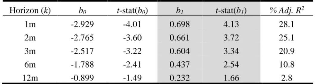
Horizon (k) b0 t-stat(b0) b1 t-stat(b1) % Adj. R2
1m -2.929 -4.01 0.698 4.13 28.1
2m -2.765 -3.60 0.661 3.72 25.1
3m -2.517 -3.22 0.604 3.34 20.9
6m -1.788 -2.41 0.437 2.54 10.8