Ray Interference: a Source of Plateaus in Deep Reinforcement Learning

(1)

Ray Interference: a Source of Plateaus in Deep

Reinforcement Learning

Tom Schaul1,*, Diana Borsa1, Joseph Modayil1and Razvan Pascanu1

1_DeepMind,*_{Corresponding author:}_{[email protected]}

Rather than proposing a new method, this paper investigates an issue present in existing learning al-gorithms. We study the learning dynamics of reinforcement learning (RL), specifically a characteristic coupling between learning and data generation that arises because RL agents control their future data distribution. In the presence of function approximation, this coupling can lead to a problematic type of ‘ray interference’, characterized by learning dynamics that sequentially traverse a number of performance plateaus, effectively constraining the agent to learn one thing at a time even when learning in parallel is better. We establish the conditions under which ray interference occurs, show its relation to saddle points and obtain the exact learning dynamics in a restricted setting. We characterize a number of its properties and discuss possible remedies.

1. Introduction

Deep reinforcement learning (RL) agents have achieved impressive results in recent years, tackling long-standing challenges in board games [38, 39], video games [23,26,45] and robotics [27]. At the same time, their learning dynamics are notoriously complex. In con-trast with supervised learning (SL), these algorithms operate on highly non-stationary data distributions that arecoupledwith the agent’s performance: an incompe-tent agent will not generate much relevant training data. This paper identifies a problematic, hitherto unnamed, issue with the learning dynamics of RL systems under function approximation (FA).

We focus on the case where the learning objective can be decomposed intomultiple components,

J := Õ

1≤k≤K Jk .

Although not always explicit, complex tasks commonly possess this property. For example, this property arises when learning about multiple tasks or contexts, when using multiple starting points, in the presence of multi-ple opponents, and in domains that contain decisions points with bifurcating dynamics. Sharing knowledge or representations between components can be benefi-cial in terms of skill reuse or generalization, and sharing seems essential to scale to complex domains. A common mechanism for sharing is a shared function approxima-tor (e.g., a neural network). In general however, the different components do not coordinate and so may compete for resources, resulting ininterference.

The core insight of this paper is that problematic learning dynamics arise when combining two algorithm properties that are relatively innocuous in isolation, the

interference caused by the different components and the coupling of the learning signal to the future behaviour of the algorithm. Combining these properties leads to a phenomenon we call‘ray interference’1:

A learning system suffers from plateaus if it has (a) negative interference between the compo-nents of its objective, and (b) coupled perfor-mance and learning progress.

Intuitively, the reason for the problem is that negative in-terference creates winner-take-all (WTA) regions, where improvement in one component forces learning to stall or regress for the other components of the objective. Only after such a dominant component is learned (and its gradient vanishes), will the system start learning about the next component. This is where the coupling of learning and performance has its insidious effect: this new stage of learning is really slow, resulting in a long plateau for overall performance (see Figure1).

We believe aspect (a) is common when using neural networks, which are known to exhibit negative interfer-ence when sharing representations between arbitrary tasks. On-policy RL exhibits coupling between perfor-mance and learning progress (b) because the improving behavior policy generates the future training data. Thus ray interference is likely to appear in the learning dy-namics of on-policy deep RL agents.

The remainder of the paper is structured to introduce the concepts and intuitions on a simple example (Sec-tion2), before extending it to more general cases in Section3. Section4discusses prevalence, symptoms,

1_{So called, due to the tentative resemblance of Figure}₁_{(top, left)}

to a batoidea (ray fish).

(2)

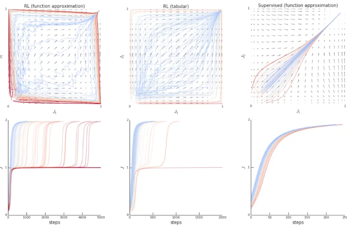
Figure 1|Illustration of ray interference in two objective component dimensionsJ1,J2.Top row:Arrows indicate the flow direction of the the learning trajectories. Each colored line is a (stochastic) sample trajectory, color-coded by performance.Bottom row:Matching learning curves for these same trajectories. Note how the trajectories that pass by the saddle points of the dynamics, at(0,1)and(1,0), in warm colors, hit plateaus and learn much slower (note that the scale of the x-axis differs per plot). Each column has a different setup.Left:RL with FA exhibits ray interference as it has both coupling and interference.Middle:Tabular RL has few plateaus because there is no interference in the dynamics.Right:Supervised learning has no plateaus even with FA interference.

interactions with different algorithmic components, as well as potential remedies.

2. Minimal, explicit setting

A minimal example that exhibits ray interference is a (K×n)-bandit problem; a deterministic contextual ban-dit withKcontexts andndiscrete actionsa∈ {1, . . . ,n}. This problem setting eliminates confounding RL ele-ments of bootstrapping, temporal structure, and stochas-tic rewards. It also permits a purely analystochas-tic treatment of the learning dynamics.

The bandit reward function is one when the action matches the context and zero otherwise: r(sk,a) :=

Ik=a whereIis the indicator function. The policy is a softmax π(a|sk) := Íexp(la,k)

a0exp(la0_,k), where l are log-its. The mapping from context to logits is parame-terised by the trainable weightsθ. The expected per-formance is the sum across contexts, J = Í

k Jk =

Í

kÍar(sk,a)π(a|sk)=Íkπ(k|sk).

A simple way to trainθ is to follow the policy gradi-ent in REINFORCE [46]. For a context-action-reward sample, this yields∆θ ∝r(sk,a)∇_θlogπ(a|sk). When

samples are generatedon-policyaccording toπ, then the expected update in contextsk is

Interference can arise from function approximation pa-rameters that are shared across contexts. To see this, represent the logits as l=Ws+b, where W is an×K

matrix, b is ann-dimensional vector, ands ∈ ZK₂ is a one-hot vector representing the current context. Note that each contextsuses a differentrowof W, hence no component of W is shared among contexts. However b is shared among contexts and this is sufficient for interference, defined as follows:

(3)

Definition 1 (Interference) We quantify thedegree of interferencebetween two components ofJas the cosine similarity between their gradients:

ρk,k0(θ):=

h∇Jk(θ),∇Jk0(θ)i

k∇Jk(θ)k k∇Jk0(θ)k

.

Qualitativelyρ=0implies no interference,ρ>0positive transfer, andρ<0negative transfer (interference).ρis bounded between−1and1.

2.1. Explicit dynamics for a(2×2)-bandit

For the two-dimensional case withK =2 contexts and

n=2 arms, we can visualize and express the full learn-ing dynamics exactly (for expected updates with an in-finite batch-size), in the continuous time limit of small step-sizes. First, we clarify our use of two kinds of derivatives that simplify our presentation. The∇ oper-ator describes a partial derivative and is usually taken with respect to the parametersθ. We omitθ whenever it is unambiguous, e.g.,∇д:=∇_θд(θ). Next, the ‘over-dot’ notation for a functionudenotes temporal deriva-tives when following the gradient∇J with respect toθ, namely Û u(θ):= lim η→0 u(θ+η∇J) −u(θ) η =h∇u,∇Ji.

LetJ1=π(a=1|s1)andJ2=π(a=2|s2). For two ac-tions, the softmax can be simplified to a simple sigmoid

σ(u)= ₁₊1_e−u. By removing redundant parameters, we

obtain:

π(a=k|sk):=σ θ1Ik=1,a=1+θ2Ik=2,a=2+θ3(2Ia=1−1) whereθ := (W1,1−W1,2,W2,1−W2,2,b1−b2) ∈ R3. This yields the following gradients:

∇J1 = ∇θπ(a=1|s1)=∇θσ(θ1+θ3) = σ(θ1+θ3)(1−σ(θ1+θ3)) d(θ1+θ3) dθ = J1(1−J1)       1 0 1       ∇J2 = J2(1−J2)       0 1 −1      

From these we compute the degree of interference

ρ := ρ1,2= h∇J1,∇J2i k∇J1k k∇J2k = J1(1−J1)J2(1−J2)(−1) J1(1−J1) √ 2·J2(1−J2) √ 2 = −1 2 , which implies a substantial amount of negative

interfer-2.2. Dynamical system

The learning dynamics follow the full gradient∇J =

∇J1+∇J2, and we examine them in the limit of small stepsizesη→0, in the coordinate system given byJ1 andJ2. The directional derivatives along∇Jfor the two componentsJ1andJ2are:

Û J1(θ) = h∇J1,∇Ji = k∇J1k2+h∇J1,∇J2i = 2J12(1−J1)2−J1(1−J1)J2(1−J2) (1) Û J2(θ) = 2J22(1−J2)2−J1(1−J1)J2(1−J2) (2) This system of differential equations has fixed points at the four corners, where(J1=0,J2=0)is unstable, (1,1)is a stable attractor (the global optimum), and (0,1)and(1,0)are saddle points; see AppendixB.1for derivations. The left of Figure1depicts exactly these dynamics.

2.3. Flat plateaus

By considering the inflection points where the learn-ing dynamics re-accelerate after a slow-down, we can characterize its plateaus, formally:

Definition 2 (Plateaus) We say that the learning dy-namics ofJ have anϵ-plateauat a pointθ if and only if

0≤ ÛJ(θ) ≤ϵ, JÜ(θ)=0, JÝ(θ)>0 .

In other words,θ is an inflection point of J where the learning curve along∇Jswitches from concave to convex. Atθ, the derivativeϵ >0characterizes the plateau’s flat-ness, characterizing how slow learning is at the slowest (nearby) point.

In our example, the acceleration is: Ü

J = h∇ ÛJ,∇Ji=(1−J1−J2)P6(J1,J2) , (3) whereP6is a polynomial of max degree 6 inJ1andJ2; see AppendixB.2for details. This implies thatJÜ=0 along the diagonal whereJ2 =1−J1, andJÜchanges sign there. We have a plateau if the sign-change is from negative to positive, see Figure2. These points lie near the saddle points and areϵ-plateaus, with their ‘flatness’ given by

ϵ =JÛ|J2=1−J1 =2J 2

1(1−J1)2 ,

which is vanishingly small near the corners. Under ap-propriate smoothness constraints onJ, the existence of anϵ-plateau slows down learning byO(1

ϵ)steps

com-pared to a plateau-free baseline; see Figure8for empir-ical results.

(4)

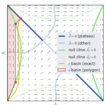
Figure 2|Bandit learning dynamics:Geometric intu-itions to accompany the derivations. The green hyper-bolae show the null clines that enclose the WTA regions. Inflection points are shown in blue, of which the solid lines are plateaus (JÝ>0), while the dashed lines are not. The orange path encloses the basin of attraction for a plateau ofϵ=0.1. The red polygon is its lower-bound approximation for which the vertices can be derived ex-plicitly (AppendixB.3).

2.4. Basins of attraction

Flat plateaus are only a serious concern if the learning trajectories are likely to pass through them. The exact basins of attraction are difficult to characterize, but some parts are simple, namely the regions where one component dominates.

Definition 3 (Winner-take-all) We denote the learning dynamics at a pointθ aswinner-take-all(WTA) if and only if

Û

Jk(θ)>0 and ∀k0,k, JÛk0(θ) ≤0 ,

that is, following the full gradient∇J only increases the kth_component.

The core property of interest for a WTA region is that for every trajectory passing through it, when the trajec-tory leaves the region, all components of the objective except for thekth_{will have decreased. In our example,} the null clines describe the WTA regions. They follow the hyperbolae:

Û

J1 = 0⇔2J1(1−J1)=J2(1−J2)

Û

J2 = 0⇔J1(1−J1)=2J2(1−J2) ,

as shown in Figure2. Armed with the knowledge of plateau locations and WTA regions, we can establish theirbasins of attraction, see Figure2and AppendixB.3, and thus the likelihood of hitting anϵ-plateau under any distribution of starting points. For distributions near the origin and uniform across angular directions, it can be shown that the chance of initializing the model in a WTA region is over 50% (AppendixB.4). Figure5

shows empirically that for initializations with low overall performance J(θ0) 1, a large fraction of learning trajectories hit (very) flat plateaus.

2.5. Contrast example: supervised learning We can obtain the explicit dynamics for a variant of the (2×2)setup where the policy is not trained by REIN-FORCE, but by supervised learning using a cross-entropy loss toward the ground-truth ideal arm, where crucially the performance-learning coupling of on-policy RL is absent:E[∆θ|sk] ∝ ∇logπ(k|sk). In this case, interfer-ence is the same as before (ρ=−1

2), but there are no saddle points (the only fixed point is the global optimum at(1,1)), nor are there any inflection points that could indicate the presence of a plateau, becauseJÜis concave everywhere (see Figure1, right, and AppendixB.5for the derivations):

Ü

Jsup = −2J1(1−J1)(1−2J1+J2)2

−2J2(1−J2)(1−2J2+J1)2≤0 . (4)

2.6. Summary: Conditions for ray interference To summarize, the learning dynamics of a(2×2)-bandit exhibit ray interference. For many initializations, the WTA dynamics pull the system into a flat plateau near a saddle point. Figures1and3 show this hinges on two conditions. The negative interference (a) is due to having multiple contexts (K >1) and a shared function approximator; this creates the WTA regions that make it likely to hit flat plateaus (left subplots).

When using a tabular representation instead (i.e., without the action-bias), there are no WTA regions, so the basins of attraction for the plateaus are smaller and do not extend toward the origin, and ray interference vanishes, see Figure1(middle subplots). On the other hand, the learning dynamics couple performance and learning progress (b) because samples are generated by the current policy. Ray interference disappears when this coupling is broken, because without the coupling, the dynamics have no saddle points or plateaus. We see this when a uniform random behavior policy is used, or when the policy is trained directly by supervised learning (Section2.5); see Figure1(right subplots).

(5)

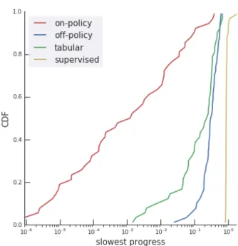
Figure 3|Likelihood of encountering a flat plateau. This plot shows on the likelihood (vertical axis) that the slowest learning progress, min| ÛJ|, along a trajec-tory is below some value—when there is a plateau, this is its flatness (horizontal axis). For example, 20% of on-policy runs (red curve) traverse a very flat plateau withϵ ≤10−5. All these results are empirical quantiles, when starting at low initial performance, J(θ0) = ₁₀K, and ignoring slow progress near the start or the opti-mum. There are four settings: ray interference (red) is a consequence of two ingredients, interference and coupling. Multiple ablations eliminate it: interference can be removed by training separate networks or using a tabular representation (green); coupling can be re-moved by off-policy RL with uniform exploration (blue) or a supervised learning setup as in Section2.5 (yel-low). One key contributing factor that impacts whether a trajectory is ‘lucky’ is whether it is initialized near the diagonal (J1(θ0) ≈J2(θ0)) or not: the more imbalanced the initial performance, the more likely it is to encounter a slow plateau.

3. Generalizations

In this section, we generalize the intuitions gained on the simple bandit example, and characterize a broader class of problems that exhibit ray interference. 3.1. Factored objectives

There is one class of learning problems that lends itself to such generalization, namely when the component updates are explicitly coupled to performance, and can be written in the following form:

∇_θJk(θ)= fk(Jk)vk(θ) (5)

where fk :R7→R+is a smooth scalar function map-ping to positive numbers that does not depend on the currentθexcept viaJk, andvk :Rd 7→Rd is a gradient vector field. Furthermore, suppose that each compo-nent is bounded: 0≤ Jk ≤ J_kmax. When the optimum is reached, there is no further learning, sofk(J_kmax)=0,

but for intermediate points learning is always possible, i.e., 0<Jk <J_kmax⇒fk(Jk)>0.

A sufficient condition for a saddle point to exist is that for one of the components there is no learning at its performance minimum, i.e.,_∃k:fk(0)=0. The reason is thatfk0(Jmax

k0 )=0, so thenJÛ=0 at any point where

all other components are fully learned.

As a first step to assess whether there exist plateaus near the saddle points, we look at the two-dimensional case. Without loss of generality, we pick f1(0) = 0 and Jmax

2 = 1. The saddle point of interest is (J1 = 0,J2 = 1), so we need to determine the sign of JÜat the two nearby points(0,1−ξ)and(ξ,1), with 0 <

ξ 1. Under reasonable smoothness assumptions, a sufficient condition for a plateau to exist between these points is that bothJÜ|_J₁₌0,J2=1−ξ < 0 and JÜ|J1=ξ,J2=1 > 0, becauseJÜhas to cross zero between them. Under certain assumptions, made explicit in our derivations in AppendixC.1, we have: Ü J_J₁₌ 0 ≈ 2f2(J2) 3_f0 2(J2)kv2k4 Ü J_J₂₌ 1 ≈ 2f1(J1) 3 f10(J1)kv1k4 ,

the sign of which only depends onf0. Furthermore, we know thatf₁0(ξ)>0 for smallξ becausef1is smooth,

f1(0) =0 and f1(ξ) > 0, and similarly f₂0(1−ξ)< 0 becausef2(1)=0 andf2(1−ξ) >0. In other words, the same condition sufficient to induce a saddle point (f1(0)=0) is also sufficient to induce plateaus nearby. Note that the approximation here comes from assuming that∇vk is small near the saddle point.

At this point it is worth restating the shape of thefk

in the bandit examples from the previous section: with the REINFORCE objective, we hadfk(u)=u(1−u)and

under supervised learning we hadfk(u)=1−u; the

extra factor ofuin the RL case is what introduced the saddle points, and its source was the (on-policy) data coupling; see Figure6for an illustration.

Ray interference requires a second ingredient besides the existence of plateaus, namely WTA regions that create the basins of attraction for these plateaus. For the saddle point at(J1=0,J2=1), the WTA region of interest is the one whereJ2dominates, i.e.,

Û

J1≤0 ⇔ h∇J1,∇Ji ≤0

⇔ f1(J1)2kv1k2+f1(J1)f2(J2)v>1v2≤0 ⇔ f1(J1)kv1k+ρ f2(J2)kv2k ≤0 .

(6)

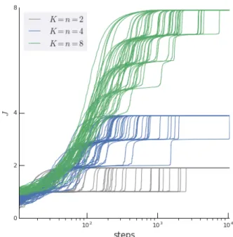
Figure 4|Learning curves when scaling up the problem dimension (jointlyK andn). We observe that theK=

8 runs go through more separate plateaus, and each plateau takes exponentially longer to overcome than the previous one (the horizontal axis is log-scale).

Of course, this can only happen if there is negative in-terference (ρ<0). If that is the case however, a WTA region necessarily exists in a strip around 0<ξ 1, becausef1being smooth means thatf1(ξ)eventually be-comes small enough for the negative term to dominate. In addition, as AppendixC.2shows, the sign change in

Ü

J occurs in the region between the null clinesJÛ1 =0 andJÛ2=0, which in turn means that for any plateau, there exist starting points inside the WTA region that lead to it.

3.2. More than two components

We have discussed conditions for saddle points to exist for any number of componentsK ≥ 2. In fact, the number of saddle points grows exponentially with the number of components that satisfy fk(0) = 0. The previous section’s arguments that establish the existence of plateaus nearby can be extended to theK >2 case as well, but we omit the details here.

Characterizing the WTA regions in higher dimensions is less straight-forward. The simple case is the ‘fully-interfering’ one, where all components compete for the same resources, and they have negative pair-wise in-terference everywhere (_∀k , k0 : ρk,k0 < 0): in this

case, the previous section’s argument can be extended to show that WTA regions must exist near the boundaries.

However, WTA is an unnecessarily strong criterion for pulling trajectories toward plateaus for ray interference:

we have seen in Figure2that the basins of attraction extend beyond the WTA region (compare green and orange), especially in the low-performance regime. For example consider three components A, B and C, where A learns first and suppresses B (as before). Now during this stage, C might behave in different ways. It could learn only partially, converge in parallel with A or be suppressed as B. When moving to stage two, once A is learned, if C has not fully converged,ray interference

dynamics can appear between B and C. Note that a critical quantity is the performance of C after stage one; this is not a trivial one to make formal statements about, so we rely on an empirical study. Figure4shows that the number of plateaus grows withKin fully-interfering scenarios. ForK =8, we observe that typically a first plateau is hit after a few components have been learned (J ≈ 3), indicating that the initialization was not in a WTA region. But after that, most learning curves look like step functions that learn one of the remaining components at a time, with plateaus in-between these stages.

A more surprising secondary phenomenon is that the plateaus seem to get exponentially worse in each stage (note the log-scale). We propose two interpretations. First, consider the two last components to be learned. They have not dominated learning forK−2 stages, all the while being suppressed by interference, and thus their performance level is very low when the last stage starts, much lower than at initialization. And as Figure5

shows, a low initial performance dramatically affects the chance that the dynamics go through a very flat plateau. Second, the length of the plateau may come from the interference of theKth_{task with all previously} learnedK−1 tasks. Basically, when starting to learn theKth_{task, a first step that improves it can negatively} interfere with the firstK−1 tasks. In a second step, these previous tasks may dominate the update and move the parameters such that they recover their performance. Thus the only changes preserved from these two tug-of-war steps are those in thenull-spaceof the firstK−1 tasks. Learning to use only that restricted capacity for taskKtakes time, especially in the presence of noise, and could thus explain that the length the plateaus grows withK.

3.3. From bandits to RL

While the bandit setting has helped ease the exposition, our aim is to gain understanding in the more general (deep) RL case. In this section, we argue that there are

someRL settings that are likely to be affected by ray in-terference. First, there are many cases where the single scalar reward objective can be seen as a composite of manyJk: the simple analogue to the contextual bandit are domains with multiple rooms, levels or opponents

(7)

(e.g., Atari games like Montezuma’s Revenge), and a competent policy needs to be good in/against many of these. The additive assumptionJ =Í_J

k may not be a perfect fit, but can be a good first-order approxima-tion in many cases. More generally, when rewards are very sparse, decompositions that split trajectories near reward events is a common approximation in hierarchi-cal RL [19,24]. Other plausible decompositions exist in undiscounted domains where each reward can be ‘collected’ just once, in which case each such reward can be viewed as a distinctJk, and the overall perfor-mance depends on how many of them the policy can collect, ignoring the paths and ordering. It is important to note that a decomposition does not have to be ex-plicit, semantic or clearly separable: in some domains, competent behavior may be well explained by a com-bination of implicit skills—and if the learning of such skills is subject to interference, then ray interference may be an issue.

Another way to explain RL dynamics from our bandit investigation is to consider that each arm is a temporally abstractoption[43], with ‘contexts’ referring to parts of state space where different options are optimal. This connection makes an earlier assumption less artificial: we assumed low initial performance in Figure3, which is artificial in a 2-armed bandit, but plausible if there is an arm for each possible option.

In RL, interference can also arise in other ways than the competition in policy space we observed for bandits. There can be competition around what to memorize, how to represent state, which options to refine, and where to improve value accuracy. These are commonly conflated in the dynamics of a shared function approx-imator, which is why we consider ray interference to apply todeepRL in particular. On the other hand, the potential for interference is also paired with the po-tential for positive transfer (ρ >0), and a number of existing techniques try to exploit this, for example by learning about auxiliary tasks [17].

Coupling can also be stronger in the RL case than for the bandit: while we considered a uniform distribution over contexts, it is more realistic to assume that the RL agent will visit some parts of state space far more often than others. It is likely to favour those where it is learning, or seeing reward already (amplifying the rich-get-richer effect). To make this more concrete, assume that the performanceJk sufficiently determines the data distribution the agent encounters, such that its effect on learning aboutJk in on-policy RL can be summarized

by the scalar functionfk(Jk)(see Section3.1), at least

in the low-performance regime. For the types of RL domains discussed above it is likely that fk(0) ≈ 0,

i.e., that very little can be learned from only the data produced by an incompetent policy—thereby inducing ray interference.

We have already alluded to the impact of on-policy versus off-policy learning: the latter is generally consid-ered to lead to a number of difficulties [42]—however, it can also reduce the coupling in the learning dynamics; see for example Figure6for an illustration of howfk

changes when mixing the soft-max policy with 10% of random actions: crucially it no longer satisfiesfk(0)=0.

This perspective that off-policy learning can induce bet-ter learning dynamics in some settings, took some of the authors by surprise.

3.4. Beyond RL

A related phenomenon to the one described here was previously reported for supervised learning by Saxe et al. [34], for the particular case ofdeep linearmodels. This setting makes it easy to analytically express the learn-ing dynamics of the system, unlike traditional neural networks. Assuming a single hidden layer deep linear model, and following the derivation in [34], under the full batch dynamics, the continuous time update rule is given by:

Û

W1 ∝ W2>(Σxy−W2W1Σxx)

Û

W2 ∝ (Σxy −W2W1Σxx)W1> ,

whereW1andW2are the weights on the first and sec-ond layer respectively (the deep linear model does not have biases),Σ_xy is the correlation matrix between the input and target, andΣ_xx is the input correlation ma-trix. Using the singular value decomposition ofΣxy

and assumingΣxx = I, they study the dynamics for each mode, and find that the learning dynamics lead to multiple plateaus, where each plateau corresponds to learning of a different mode. Modes are learned sequen-tially, starting with the one corresponding to the largest singular value (see the original paper for full details). Learning each mode of theΣxy has its analogue in the different objective componentsJk in our notation. The learning curves showed in [34] resemble those observed in Figures1and4, and their Equation (5) describing the per-mode dynamics has a similar structure to our Equations1and2.

Our intuition on how this similarity comes about is speculative. One could view the hidden representation as the input of the top part of the model (W2). Now from the perspective of that part, the input distribution is

non-stationarybecause the hidden features (defined by

W1) change. Moreover, this non-stationarity is coupled to what has been learned so far, because the error is propagated through the hidden features intoW1. If the system is initialized such that the hidden units are correlated, then learning the different modes leads to a competition over the same representation or resources. The gradient is initially dominated by the mode with

(8)

the largest singular value and therefore the changes to the hidden representation correspond features needed to learn this mode only. Once the loss for the dominant mode converges, symmetry-breaking can happen, and some of the hidden features specialize to represent the second mode. This transition is visible as a plateau in the learning curve.

While this interpretation highlights the similarities with the RL case via coupling and competition of re-sources, we want to be careful to highlight that both of these aspects work differently here. The coupling does not have the property that low performance also slows down learning (Section3.1). It is not clear whether the modes exhibit negative interference where learning about one mode leads to undoing progress on another one, it could be more akin to the magnitude of the noise of the larger mode obfuscating the signal on how to improve the smaller one.

Their proposed solution is an initialization scheme that ensures all variations of the data are preserved when going through the hierarchy, in line with previous initialization schemes [10,20], which leads to symme-try breaking and reduces negative interference during learning. Unfortunately, as this solution requires access to the entire dataset, it does not have a direct analogue in RL where the relevant states and possible rewards are not available at initialization.

Multi-task versus continual learning Our investiga-tion has natural connecinvestiga-tions to the field ofmulti-task

learning (be it for supervised or RL tasks [25, 31]), namely by considering that the multitask objective is additive over oneJk per task. It is not uncommon to

observetask dominancein this scenario (learning one task at a time [12]), and our analysis suggests possi-ble reasons why tasks are sometimes learned sequen-tially despite the setup presenting them to the learning system all at once. On the other hand, we know that deep learning struggles with fully sequential settings, as incontinual learningorlife-long learning[30,36,40], one of the reasons being that the neural network’s ca-pacity can be exhausted prematurely (saturated units), resulting in an agent that can never reach its full poten-tial. So this raises the questions why current multi-task techniques appear to be so much more effective than continual learning, if they implicitly produce sequen-tial learning? One hypothesis is that the potensequen-tial tug-of-war dynamics that happen when moving from one component to another are akin to rehearsal methods for continual learning, help split the representation, and allowing room for learning the features required by the next component. Two other candidates could be that the implicit sequencing produces better task orderings and timings than external ones, or the notion that what is sequenced are not tasks themselves but skills that are

useful across multiple tasks. But primarily, we profess our ignorance here, and hope that future work will elu-cidate this issue, and lead to significant improvements in continual learning along the way.

4. Discussion

How prevalent is it? Ray interference does not re-quire an explicit multi-task setting to appear. A given single objective might be internally composed of sub-tasks, some of which have negative interference. We hypothesize, for example, that performance plateaus observed in Atari [e.g.14,23] might be due to learning multiple interfering skills (such as picking up pellets, avoiding ghosts and eating ghosts in Ms PacMan). Con-versely, some of the explicit multi-task RL setups appear not to suffer from visible plateaus [e.g.6]. There is a long list of reasons for why this could be, from the task not having interfering subtasks, positive transfer outweighing negative interference, the particular archi-tecture used, or population based training [16] hiding the plateaus through reliance on other members of the population. Note that the lack of plateaus does not exclude the sequential learning of the tasks. Finally, ray interference might not be restricted to RL settings. Similar behaviour has been observed for deep (linear) models [34], though we leave developing the relation-ship between these phenomena as future work.

How to detect it? Ray interference is straight-forward to detect if the componentsJkare known (and

appropri-ate), by simply monitoring whether progress stalls on some components while others learn, and then picks up later. It can be verified by training a separate network for each component from the same (fixed) data. In the more general case, where only the overall objectiveJ is known, a first symptom to watch out for is plateaus in the learning curve ofindividual runs, as plateaus tend to be averaged out when curves aggregated across many runs. Once plateaus have been observed, there are two types of control experiments: interference can be reduced by changing the function approximator (capac-ity or structure), or coupling can be reduced by fixing the data distribution or learning more off-policy. If the plateaus dissipate under these control experiments, they were likely due to ray interference.

What makes it worse? For simplicity, we have ex-amined only one type of coupling, via the data gener-ated from the current policy, but there can be other sources. When contexts/tasks are not sampled uni-formly but shaped intocurriculabased on recent learn-ing progress [8,11], this amplifies the winner-take-all dynamics. Also, using temporal-difference methods that

(9)

bootstrapfrom value estimates [42] may introduce a form of coupling where the values improve faster in regions of state space that already have accurate and consistent bootstrap targets. A form of coupling that operates on the population level is connected to selec-tive pressure [16]: the population member that initially learns fastest can come to dominate the population and reducediversity—favoring one-trick ponies in a multi-player setup, for example.

What makes it better? There are essentially three approaches: reduce interference, reduce coupling, or tackle ray interfere head-on. Assuming knowledge of the components of the objective, the multi-task litera-ture offers a plethora of approaches to avoid negative interference, from modular or multi-head architectures to gating or attention mechanisms [3,7,32,37,41,44]. Additionally, there are methods that prevent the inter-ference directly at the gradient level [5,47], normalize the scales of the losses [15], or explicitly preserve ca-pacity for late-learned subtasks [18]. It is plausible that following thenaturalgradient [1,28] helps as well, see for example [4] (their figures 9b and 11b) for prelimi-nary evidence. When the components are not explicit, a viable approach is to use population-based methods that encourage diversity, and exploit the fact that dif-ferent members will learn about difdif-ferent implicit com-ponents; and that knowledge can be combined [e.g., using a distillation-based cross-over operator,9]. A possibly simpler approach is to rely on innovations in deep learning itself: it is plausible that deep networks with ReLU non-linearities and appropriate initialization schemes [13] implicitly allow units to specialize. Note also that the interference can bepositive, learning one component helps on others (e.g., via refined features). Coupling can be reduced by introducing elements of off-policy learning that dilutes the coupled data distri-bution with exploratory experience (or experience from other agents), rebalancing the data distribution with a suitable form of prioritized replay [35] or fitness shar-ing [33], or by reward shaping that makes the learning signal less sparse [2]. A generic type of decoupling solution (when components are explicit) is to train sep-arate networks per component, anddistillthem into a single one [21,32]. Head-on approaches to alleviate ray interference could draw from the growing body of continual learning techniques [22,29,30,36,40].

5. Conclusion

This paper studied ray interference, an issue that can stall progress in reinforcement learning systems. It is a combination of harms that arise from (a) conflicting feedback to a shared representation from multiple ob-jectives, and (b) changing the data distribution during

policy improvement. These harms are much worse when combined, as they cause learning progress to stall, be-cause the expected learning update drags the learning system towards plateaus in gradient space that require a long time to escape. As such, ray interference is not restricted to deep RL (a bias unit weight shared across different actions in a linear model suffices), but rather it shows how harmful forms of interference, similar to those studied in deep learning, can arise naturally within reinforcement learning. This initial investigation stops short of providing a full remedy, but it sheds light onto these dynamics, improves understanding, teases out some of the key factors, and hints at possible direc-tions for solution methods.

Zooming out from the overall tone of the paper, we want to highlight that plateaus are not omnipresent in deep RL, even in complex domains. Their absence might be due to the many commonly used practical innovations that have been proposed for stability or performance reasons. As they affect the learning dynamics, they could indeed alleviate ray interference as a secondary effect. It may therefore be worth revisiting some of these methods, from a perspective that sheds light on their relation to phenomena like ray interference.

References

[1] S.-I. Amari. Natural gradient works efficiently in learning. Neural computation, 10(2):251–276, 1998.

[2] J. A. Arjona-Medina, M. Gillhofer, M. Widrich, T. Unterthiner, J. Brandstetter, and S. Hochreiter. RUDDER: Return decomposition for delayed re-wards.arXiv preprint arXiv:1806.07857, 2018. [3] J. Chung, C. Gulcehre, K. Cho, and Y. Bengio.

Empirical evaluation of gated recurrent neural networks on sequence modeling. arXiv preprint arXiv:1412.3555, 2014.

[4] R. Dadashi, A. A. Taïga, N. L. Roux, D. Schu-urmans, and M. G. Bellemare. The value func-tion polytope in reinforcement learning. CoRR, abs/1901.11524, 2019.

[5] Y. Du, W. M. Czarnecki, S. M. Jayakumar, R. Pas-canu, and B. Lakshminarayanan. Adapting auxil-iary losses using gradient similarity.arXiv preprint arXiv:1812.02224, 2018.

[6] L. Espeholt, H. Soyer, R. Munos, K. Simonyan, V. Mnih, T. Ward, Y. Doron, V. Firoiu, T. Harley, I. Dunning, et al. IMPALA: Scalable distributed Deep-RL with importance weighted actor-learner architectures. arXiv preprint arXiv:1802.01561, 2018.

(10)

[7] C. Fernando, D. Banarse, C. Blundell, Y. Zwols, D. Ha, A. A. Rusu, A. Pritzel, and D. Wierstra. Path-net: Evolution channels gradient descent in super neural networks.arXiv preprint arXiv:1701.08734, 2017.

[8] S. Forestier and P.-Y. Oudeyer. Modular active curiosity-driven discovery of tool use. InIntelligent Robots and Systems (IROS), 2016 IEEE/RSJ Inter-national Conference on, pages 3965–3972. IEEE, 2016.

[9] T. Gangwani and J. Peng. Genetic policy optimiza-tion.arXiv preprint arXiv:1711.01012, 2017. [10] X. Glorot and Y. Bengio. Understanding the

dif-ficulty of training deep feedforward neural net-works. InIn Proceedings of the International Con-ference on Artificial Intelligence and Statistics (AIS-TATS’10). Society for Artificial Intelligence and Statistics, 2010.

[11] A. Graves, M. G. Bellemare, J. Menick, R. Munos, and K. Kavukcuoglu. Automated curriculum learning for neural networks. arXiv preprint arXiv:1704.03003, 2017.

[12] M. Guo, A. Haque, D.-A. Huang, S. Yeung, and L. Fei-Fei. Dynamic task prioritization for mul-titask learning. In Proceedings of the European Conference on Computer Vision (ECCV), pages 270– 287, 2018.

[13] K. He, X. Zhang, S. Ren, and J. Sun. Delv-ing deep into rectifiers: SurpassDelv-ing human-level performance on imagenet classification. CoRR, abs/1502.01852, 2015.

[14] M. Hessel, J. Modayil, H. Van Hasselt, T. Schaul, G. Ostrovski, W. Dabney, D. Horgan, B. Piot, M. Azar, and D. Silver. Rainbow: Combining im-provements in deep reinforcement learning. In

Thirty-Second AAAI Conference on Artificial Intelli-gence, 2018.

[15] M. Hessel, H. Soyer, L. Espeholt, W. Czarnecki, S. Schmitt, and H. van Hasselt. Multi-task deep reinforcement learning with popart.arXiv preprint arXiv:1809.04474, 2018.

[16] M. Jaderberg, V. Dalibard, S. Osindero, W. M. Czarnecki, J. Donahue, A. Razavi, O. Vinyals, T. Green, I. Dunning, K. Simonyan, et al. Pop-ulation based training of neural networks. arXiv preprint arXiv:1711.09846, 2017.

[17] M. Jaderberg, V. Mnih, W. M. Czarnecki, T. Schaul, J. Z. Leibo, D. Silver, and K. Kavukcuoglu. Rein-forcement learning with unsupervised auxiliary tasks. arXiv preprint arXiv:1611.05397, 2016. [18] J. Kirkpatrick, R. Pascanu, N. Rabinowitz, J.

Ve-ness, G. Desjardins, A. A. Rusu, K. Milan, J. Quan,

T. Ramalho, A. Grabska-Barwinska, et al. Over-coming catastrophic forgetting in neural networks.

Proceedings of the national academy of sciences, 114(13):3521–3526, 2017.

[19] T. Lane and L. P. Kaelbling. Toward hierarchical decomposition for planning in uncertain environ-ments. InProceedings of the 2001 IJCAI workshop on planning under uncertainty and incomplete in-formation, pages 1–7, 2001.

[20] Y. LeCun, L. Bottou, G. B. Orr, and K.-R. Müller. Efficient backprop. In G. Montavon, G. B. Orr, and K.-R. Müller, editors,Neural Networks: Tricks of the Trade, volume 7700 ofLecture Notes in Computer Science, pages 9–48. Springer, 1998.

[21] D. Lopez-Paz, L. Bottou, B. Schölkopf, and V. Vap-nik. Unifying distillation and privileged informa-tion. arXiv preprint arXiv:1511.03643, 2015. [22] D. Lopez-Paz and M. A. Ranzato. Gradient

episodic memory for continual learning. In Ad-vances in Neural Information Processing Systems, pages 6467–6476, 2017.

[23] V. Mnih, K. Kavukcuoglu, D. Silver, A. A. Rusu, J. Veness, M. G. Bellemare, A. Graves, M. Ried-miller, A. K. Fidjeland, G. Ostrovski, S. Petersen, C. Beattie, A. Sadik, I. Antonoglou, H. King, D. Ku-maran, D. Wierstra, S. Legg, and D. Hassabis. Human-level control through deep reinforcement learning. Nature, 518(7540):529–533, 2015. [24] A. W. Moore, L. Baird, and L. P. Kaelbling.

Multi-value-functions: Effcient automatic action hier-archies for multiple goal MDPs. In Proceedings of the international joint conference on artificial intelligence, pages 1316–1323, 1999.

[25] J. Oh, S. Singh, H. Lee, and P. Kohli. Zero-shot task generalization with multi-task deep reinforcement learning. InProceedings of the 34th International Conference on Machine Learning-Volume 70, pages 2661–2670. JMLR. org, 2017.

[26] OpenAI. Openai five. https://blog.openai.com/ openai-five/, 2018.

[27] OpenAI, M. Andrychowicz, B. Baker, M. Chociej, R. Józefowicz, B. McGrew, J. W. Pachocki, J. Pa-chocki, A. Petron, M. Plappert, G. Powell, A. Ray, J. Schneider, S. Sidor, J. Tobin, P. Welinder, L. Weng, and W. Zaremba. Learning dexterous in-hand manipulation. CoRR, abs/1808.00177, 2018.

[28] J. Peters, S. Vijayakumar, and S. Schaal. Natural actor-critic. InEuropean Conference on Machine Learning, pages 280–291. Springer, 2005. [29] M. Riemer, I. Cases, R. Ajemian, M. Liu, I. Rish,

(11)

Y. Tu, , and G. Tesauro. Learning to learn without forgetting by maximizing transfer and minimiz-ing interference. InInternational Conference on Learning Representations, 2019.

[30] M. B. Ring. Continual learning in reinforcement environments. PhD thesis, University of Texas at Austin Austin, Texas 78712, 1994.

[31] S. Ruder. An overview of multi-task learn-ing in deep neural networks. arXiv preprint arXiv:1706.05098, 2017.

[32] A. A. Rusu, S. G. Colmenarejo, C. Gulcehre, G. Desjardins, J. Kirkpatrick, R. Pascanu, V. Mnih, K. Kavukcuoglu, and R. Hadsell. Policy distillation.

arXiv preprint arXiv:1511.06295, 2015.

[33] B. Sareni and L. Krahenbuhl. Fitness sharing and niching methods revisited. IEEE transactions on Evolutionary Computation, 2(3):97–106, 1998. [34] A. M. Saxe, J. L. McClelland, and S. Ganguli. Exact

solutions to the nonlinear dynamics of learning in deep linear neural networks. ICLR, 2014. [35] T. Schaul, J. Quan, I. Antonoglou, and D.

Sil-ver. Prioritized experience replay. arXiv preprint arXiv:1511.05952, 2015.

[36] T. Schaul, H. van Hasselt, J. Modayil, M. White, A. White, P. Bacon, J. Harb, S. Mourad, M. G. Bellemare, and D. Precup. The Barbados 2018 list of open issues in continual learning. CoRR, abs/1811.07004, 2018.

[37] N. Shazeer, A. Mirhoseini, K. Maziarz, A. Davis, Q. Le, G. Hinton, and J. Dean. Outrageously large neural networks: The sparsely-gated mixture-of-experts layer. arXiv preprint arXiv:1701.06538, 2017.

[38] D. Silver, A. Huang, C. J. Maddison, A. Guez, L. Sifre, G. van den Driessche, J. Schrittwieser, I. Antonoglou, V. Panneershelvam, M. Lanctot, S. Dieleman, D. Grewe, J. Nham, N. Kalchbrenner, I. Sutskever, T. Lillicrap, M. Leach, K. Kavukcuoglu, T. Graepel, and D. Hassabis. Mastering the game of Go with deep neural networks and tree search.

Nature, 529:484–503, 2016.

[39] D. Silver, T. Hubert, J. Schrittwieser, I. Antonoglou, M. Lai, A. Guez, M. Lanctot, L. Sifre, D. Kumaran, T. Graepel, et al. A general reinforcement learn-ing algorithm that masters chess, shogi, and go through self-play.Science, 362(6419):1140–1144, 2018.

[40] D. L. Silver, Q. Yang, and L. Li. Lifelong machine learning systems: Beyond learning algorithms. In

2013 AAAI spring symposium series, 2013. [41] M. F. Stollenga, J. Masci, F. Gomez, and J.

Schmid-huber. Deep networks with internal selective atten-tion through feedback connecatten-tions. InAdvances in neural information processing systems, pages 3545–3553, 2014.

[42] R. S. Sutton and A. G. Barto. Reinforcement learn-ing: An introduction. MIT press, 2018.

[43] R. S. Sutton, D. Precup, and S. Singh. Between mdps and semi-mdps: A framework for temporal abstraction in reinforcement learning. Artificial intelligence, 112(1-2):181–211, 1999.

[44] C.-Y. Tsai, A. M. Saxe, and D. Cox. Tensor switch-ing networks. In D. D. Lee, M. Sugiyama, U. V. Luxburg, I. Guyon, and R. Garnett, editors, Ad-vances in Neural Information Processing Systems 29, pages 2038–2046. Curran Associates, Inc., 2016. [45] O. Vinyals, I. Babuschkin, J. Chung, M. Mathieu, M. Jaderberg, W. M. Czarnecki, A. Dudzik, A. Huang, P. Georgiev, R. Powell, T. Ewalds, D. Horgan, M. Kroiss, I. Danihelka, J. Agapiou, J. Oh, V. Dalibard, D. Choi, L. Sifre, Y. Sulsky, S. Vezhnevets, J. Molloy, T. Cai, D. Budden, T. Paine, C. Gulcehre, Z. Wang, T. Pfaff, T. Pohlen, Y. Wu, D. Yogatama, J. Cohen, K. McKinney, O. Smith, T. Schaul, T. Lillicrap, C. Apps, K. Kavukcuoglu, D. Hassabis, and D. Silver. AlphaStar: Mastering the Real-Time Strategy Game StarCraft II. https://deepmind.com/blog/ alphastar-mastering-real-time-strategy-game-starcraft-ii/, 2019.

[46] R. J. Williams. Simple statistical gradient-following algorithms for connectionist reinforce-ment learning.Machine learning, 8(3-4):229–256, 1992.

[47] D. Yin, A. Pananjady, M. Lam, D. S. Papailiopou-los, K. Ramchandran, and P. Bartlett. Gradient diversity empowers distributed learning. CoRR, abs/1706.05699, 2017.

Acknowledgements

We thank Hado van Hasselt, David Balduzzi, Andre Barreto, Claudia Clopath, Arthur Guez, Simon Osin-dero, Neil Rabinowitz, Junyoung Chung, David Silver, Remi Munos, Alhussein Fawzi, Jane Wang, Agnieszka Grabska-Barwinska, Dan Horgan, Matteo Hessel, Shakir Mohamed and the rest of the DeepMind team for helpful comments and suggestions.

(12)

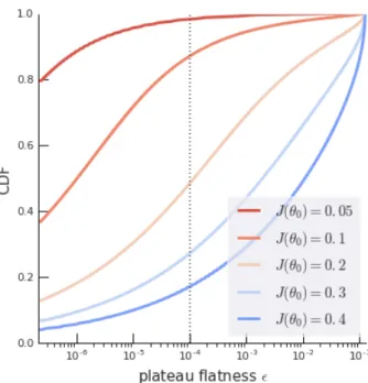
Figure 5|Basins of attraction, for plateaus of differentϵ, and for different levels of initial performanceJ(θ0), under deterministic dynamics. The dashed line indicates the typicalϵfor which learning is 10 times slower than necessary (see Figure8), so for example half of the trajectories initialized atJ(θ0)=0.2 hit such a flat plateau.

A. Additional results

We investigated numerous additional variants of the basic bandit setup. In each case, we summarize the results by the probabilities that a plateau ofϵor worse is encountered, as in Figure5. We quantify this by computing the slowest progress along the learning curve (not near the start nor the optimum), normalized to factor out the step-size. If not mentioned otherwise, we use the following settings across these experiments:K =2,n=2, low initial performanceJ(θ0) = ₁₀K, step-sizeη= 0.1, and batch-sizeK (exactly 1 per context). Learning runs are stopped near the global optimum, whenJ ≥K−0.1, or afterN =105samples.

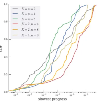
We can quantify the insights of Section3.2by measuring the flatness of theworstplateau in a learning curve that generally has more than one. Figure7gives results that validate the qualitative insights, when increasingKandn

jointly. Note that only scaling upnactually makes the problem easier (when controlling for initial performance), because the actionsK <i ≤nare disadvantageous in all contexts, so there is some positive transfer through their action biases.

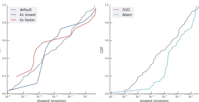
We looked at the influence of some architectural choices, using deep neural networks to parameterize the policy. It turns out that deeper or wider MLPs do not qualitatively change the dynamics from the simple setup in Section2. Figure9illustrates some of the effects of learning rates and optimizer choices.

B. Detailed derivations (bandit)

B.1. Fixed point analysis

The Jacobian with respect toJ1,J2is

−2J1+1 J2− 1₂

J1−1₂ −2J2+1

(13)

Figure 6|Plot of the scalar coupling functionsf(Jk)of Equation (5) (see Section3.1). It highlights the U-shape

for on-policy REINFORCE (red), in contrast to a supervised learning setup (green, see Section2.5). In orange, it illustrates how thef(0)=0 condition no longer holds when using off-policy data, in this case, mixing 90% of on-policy data with 10% of uniform random data.

Figure 7|Likelihood of encountering a plateau for different numbers of contextsK and actionsn(same type of plot than Figure3). Note how the positive transfer from spurious actions (whenK <n, warm colors) helps performance.

(14)

Figure 8|Relation betweenϵof the traversed plateau, and the number of steps along a trajectory from near(0,0) to near(1,1). The dashed line (‘balanced’) corresponds to trajectories that follow the diagonal (J1=J2) and don’t encounter a plateau. Note that forϵ ≈10−4, the deterministic learning trajectories are 10 times slower than a diagonal trajectory (warm colors in Figure1).

Figure 9|Likelihood of encountering a bad plateau (same type of plot than Figure3).Left:Comparison between step-sizes.Right:Comparison between optimizers.

(15)

fixed point trace determinant type 0,0 2 5₄ unstable 0,1 0 −5 4 saddle 1,0 0 −5 4 saddle 1,1 -2 5₄ stable B.2. Derivation ofJÜfor RL

We characterize theaccelerationof the learning dynamics, as: Ü J := lim η→0 Û J(θ+η∇J) − ÛJ(θ) η = h∇ ÛJ,∇Ji = h∇[2J₁2(1−J1)2−2J1(1−J1)J2(1−J2)+2J22(1−J2)2],∇Ji = h4J1(1−J1)(1−2J1)∇J1+4J2(1−J2)(1−2J2)∇J2 −2J1(1−J1)(1−2J2)∇J2−2J2(1−J2)(1−2J1)∇J1,∇J1+∇J2i = 2(1−2J1)[2J1(1−J1) −J2(1−J2)]k∇J1k2+2(1−2J2)[−J1(1−J1)+2J2(1−J2)]k∇J2k2 +2[(1−2J1)[2J1(1−J1) −J2(1−J2)]+(1−2J2)[−J1(1−J1)+2J2(1−J −2)]]h∇J1,∇J2i = 4(1−2J1)(2J1−J2)J12+4(1−2J2)(2J2−J1)J12−2J1J2[(1−2J1)(2J1−J2)+(1−2J2)(2J2−J1)] = 2(1−J1−J2) −8J16+8J 5 1J2+20J15−20J 4 1J2−16J 4 1 −2J 3 1J 3 2 +3J 3 1J 2 2 +15J 3 1J2+4J13+3J 2 1J 3 2 −4J₁2J₂2−3J₁2J2+8J1J25−20J1J24+15J1J23−3J1J22−8J 6 2 +20J 5 2 −16J 4 2+4J 3 2 := (1−J1−J2)P6(J1,J2) ,

This implies thatJÜ=0 along the diagonal whereJ2=1−J1, andJÜchanges sign there. We have a plateau if the sign-change is from negative to positive, in other words, wherever

P6(J1,1−J1) ≤0 ⇔ −(J1−1)2J12(30J12−30J1+7) ≤0 ⇔ J1∈ " 0,15− √ 15 30 # orJ1∈ " 15+√15 30 ,1 # ,

C. Derivations for factored objectives case

C.1. Derivation ofJÜ

We consider objectives where each component is smooth, and can be written in the following form: ∇θJk(θ) = fk(Jk)vk(θ)

wherefk :R7→R+is a scalar function mapping to positive numbers that doesn’t depend on currentθ except via

Jk andvk :Rd 7→Rd. We further assume that each component is bounded: 0≤ Jk ≤ J_kmax. When the optimum is reached, there is no further learning, sofk(J_kmax)=0, but for intermediate points learning is always possible, i.e., 0< Jk < J_kmax⇒ fk(Jk)>0.

(17)

If the above conditions hold, then these are sufficient conditions to show that the combined objectiveJadmits an

ϵ-plateau as defined in Definition 2. Moreover,Jwill exhibit the saddle points atJ =(0,Jmax)andJ =(Jmax,0).

ρ = h∇J1,∇J2i k∇J1k k∇J2k = v₁>v2 kv1k kv2k Û J1 = h∇J1,∇Ji=kv1k2f1(J1)2+ρkv1k kv2kf1(J1)f2(J2) = kv1kf1(J1) [kv1kf1(J1)+ρkv2kf2(J2)] Û J = h∇J,∇Ji=h∇J1+∇J2,∇J1+∇J2i = kv1k2f1(J1)2+kv2k2f2(J2)2+2ρkv1k kv2kf1(J1)f2(J2) = v₁>v1f1(J1)2+v2>v2f2(J2)2+2f1(J1)f2(J2)v>1v2 ∇ ÛJ = 2kv1k2f10(J1)f1(J1)∇J1+2kv2k2f20(J2)f2(J2)∇J2+2ρkv1k kv2kf10(J1)f2(J2)∇J1 +2ρkv1k kv2kf20(J2)f1(J1)∇J2+2f1(J1)2v>1∇v1+2f2(J2)2v2>∇v2 +2f1(J1)f2(J2)v>2∇v1+2f1(J1)f2(J2)v1>∇v2

For the special caseJÜ|J1=0where f1(J1)= f1(0)=0, the majority of terms in the expression vanish: ∇ ÛJ_J₁₌₀ = 2kv2k2f20(J2)f2(J2)∇J2+2f2(J2)2v>2∇v2 and Ü J_J₁₌₀ = h∇ ÛJ,∇J1+∇J2i = h2kv2k2f20(J2)f2(J2)∇J2+2f2(J2)2v2>∇v2,∇yi = 2kv2k4f20(J2)f2(J2)3+2f2(J2)3v2>∇v2v2

If we assume that the∇vk = dv_dθk terms are negligibly small near the saddle points, then we obtain Ü

J_J₁₌

0 ≈ 2kv2k 4_f0

2(J2)f2(J2)3 By symmetry, the result forJÜ|_J₂₌1is very similar.

C.2. Connecting the WTA region and the plateau

Further, when ignoring the∇vk = dv_dθk terms, we get the general from

∇ ÛJ = 2kv1k(kv1kf1(J1)+ρkv2kf2(J2))f10(J1)∇J1+2kv2k(kv2kf2(J2)+ρkv1kf1(J1))f20(J2)∇J2 = 2 JÛ1 f1(J1) f10(J1)∇J1+2 Û J2 f2(J2) f20(J2)∇J2 Ü J = 2 JÛ1 f1(J1) f10(J1)k∇J1k2+2 Û J2 f2(J2) f20(J2)k∇J2k2+2 _Û J1 f1(J1) f10(J1)+ Û J2 f2(J2) f20(J2) ∇J1>∇J2 = 2kv1k2JÛ1f1(J1)f10(J1)+2kv2k2JÛ2f2(J2)f20(J2)+2ρkv1k kv2k[ ÛJ1f2(J2)f10(J1)+JÛ2f1f20(J2)] = 2JÛ1f10(J1)kv1k(kv1kf1(J1)+ρkv2kf2(J2))+. . . = 2f 0 1(J1) f1(J1) ( ÛJ1)2+2 f₂0(J2) f2(J2) ( ÛJ2)2

From this we can deduce that the sign change inJÜmust occur in the region between the null clinesJÛ1=0 and Û